Observing relationships between sediment-laden meltwater plumes, glacial runoff and a retreating terminus at Blomstrandbreen, Svalbard

ABSTRACT

Sediment-laden meltwater plumes are a common occurrence at the margins of marine-terminating glaciers in Svalbard and are useful proxies for inferring the glacial hydrological system and meltwater runoff. Plumes can influence calving rates, marine biogeochemistry and fjord circulation. However, little is known about how their dynamics will evolve in a warmer, wetter Arctic with increasing melt rates and retreating glacier margins. To determine the temporal magnitude and frequency evolution of sediment-laden meltwater plumes, we manually delineated plume outlines in every available Sentinel-2 image at Blomstrandbreen, Kongsfjorden, Svalbard, between 2016 and 2021. While the frequency of plumes upwelling on the fjord surface remained stable in each melt season, their surface area increased significantly by almost an order of magnitude between the beginning and end of the study period, owing primarily to glacial runoff. This significant change was a result of several large plumes (>2 km²) mapped in 2020 and 2021. The rate of glacier terminus change throughout the study period has little-to-no influence on plume surface area. However, a notable event concerning the terminus retreating into an overdeepening between 2017 and 2018 may have impacted plume magnitude, allowing for larger plume migration across the calving front after 2018. Seasonal supraglacial lakes on Blomstrandbreen are found to be small in both area and volume which have limited influence on plumes surfacing between 2016-2021. Our findings suggest with increased runoff, plumes upwelling at the glacier terminus may increase in size, transporting greater volumes of sediment into the surrounding local marine environment. These changes could be exacerbated by projected increases in glacier mass loss and retreat expected to occur across Svalbard throughout this century and beyond, making the study of plumes and their impacts key to constraining the transport of water and sediment from a terrestrial to a marine environment as demonstrated at Blomstrandbreen.

KEYWORDS:

• Marine-terminating glacier
• sediment-laden meltwater plume
• plume
• Svalbard
• Sentinel-2
• remote sensing

1. Introduction

The Arctic is warming between two and six times faster than the global average, resulting in mass loss and retreat at glaciers and ice caps (e.g. Wawrzyniak and Osuch 2020). In the period between 2006 and 2015, Arctic land ice contributed 12.4 mm sea level equivalent per year, a figure that has been increasing in recent years (Box et al. 2018). Continued warming in the Arctic impacts marine-terminating glaciers which are highly sensitive to both increasing air and ocean temperatures, which in turn can alter their behaviour (Carr, Stokes, and Vieli 2013). At the ice-bed interface, meltwater directed from the supraglacial and englacial drainage systems can be transported through a complex subglacial network to the ice margin, with large volumes of water entraining sediment that later upwells as buoyant sediment-laden meltwater plumes upon evacuation (Hewitt 2020; How et al. 2017). Sediment plumes can surface at multiple locations across glacier calving fronts, and depending on their magnitude extend substantial distances into fjord or coastal environments (Meslard et al. 2018). The location of sediment-laden meltwater plumes can influence calving and submarine melt rates at marine-terminating glaciers (Carroll et al. 2016; Schild et al. 2018), but can also impact fjord circulation (Everett et al. 2018; Torsvik et al. 2019), marine biogeochemistry (Hopwood et al. 2020), glaciomarine sedimentation (Kehrl et al. 2011), and marine and bird life (Lydersen et al. 2014). Hereafter when referring to the surfacing of sediment-laden glacial meltwater on the fjord surface, the term ‘plume’ is used.

Much of our knowledge of plumes exists from numerical modelling (e.g. Mugford and Dowdeswell 2011; Slater et al. 2017), in-situ sampling of suspended sediments (e.g. Schild et al. 2017; Tallentire et al. 2022), or through oceanographic data collected in locations proximal to, but not directly at glacier fronts (e.g. Trusel et al. 2010). While remote sensing observations of surface plumes may yield insights into their controls and variability, the acquisition of cloud-free imagery is challenging in Arctic maritime regions, particularly Svalbard (e.g. Marshall, Dowdeswell, and Rees 1994; Marshall, Rees, and Dowdeswell 1993; Østby, Schuler, and Westermann 2014). However, in more recent years a greater number of higher temporal and spatial resolution optical data from research and commercial satellites, such as Sentinel-2, and Planet Labs, have improved coverage of the region, giving greater opportunities for understanding how plumes vary through space and time.

Previous remote sensing studies have used a range of different data and techniques to better constrain the characteristics of plumes during the melt season (e.g. Chu et al. 2012). In Greenland, many studies have focussed on Qinnguata Kuussua (Watson River) which drains a ~ 66,000 km² hydrologic basin on the southwest margin of the ice sheet (Chu et al. 2009, 2012; McGrath et al. 2010; van as et al. 2018). Other studies have focused on Greenland’s plumes draining land- and marine-terminating sectors of the ice sheet (e.g. Hudson et al. 2014; Tedstone and Arnold 2012). Similar remote sensing-based plume investigations within the Arctic and pan-Arctic region have taken place in Iceland (e.g. Hodgkins et al. 2016) and Svalbard (e.g. Schild et al. 2017). Plumes have been studied at a number of locations across the Svalbard archipelago, to: (i) determine volumes of meltwater being delivered to fjords by marine-terminating glaciers (Darlington 2015), (ii) better understand plume distribution, and therefore the stability of an ice cap (Dowdeswell et al. 2015); and (iii) calculate sedimentation rates at an ice front (Kehrl et al. 2011). Primarily, these studies have made use of high temporal, low spatial resolution data, such as Moderate Resolution Imaging Spectroradiometer (MODIS) bands at 250 and 500 m resolution (e.g. Chu et al. 2012), often only using higher spatial resolution data, e.g. Landsat 7 ETM+ (30 m, 15 m with panchromatic band) or ASTER (15 m) for validation purposes.

This study presents a remote sensing approach to the manual delineation of plumes at Blomstrandbreen, Svalbard, to determine their dynamics and characteristics by analysing Sentinel-2 imagery (10 m spatial resolution) between 2016 and 2021. The aim of this paper was to assess the feasibility of deriving a seasonal time series of plume outlines within in the Google Earth Engine Digitisation Tool (GEEDiT; Lea 2018) to better understand how these features are changing through both space and time. We also analysed whether the magnitude and frequency of these plumes changed through time and consequently considered the influence of boundary conditions such as: glacial runoff, glacier terminus change and seasonal supraglacial lake evolution.

2. Study area

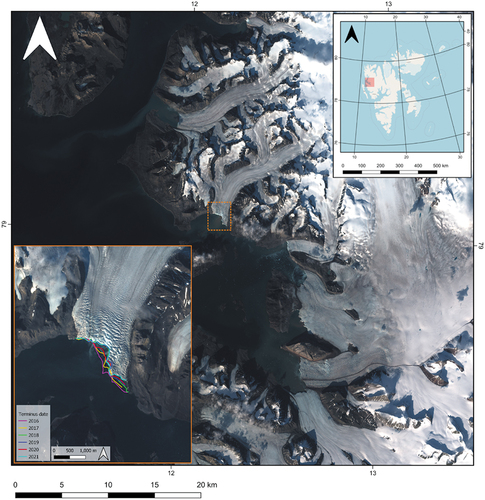
Blomstrandbreen is an 18 km long partially marine-terminating glacier which covers an ice surface area of ~80 km² and is fed by a number of tributary glaciers that results in a calving front width between 2.5–3.0 km (Burton et al. 2016; Sund and Eiken 2010) (Figure 1). The glacier flows in a south westerly direction where it drains into the northern side of Kongsfjorden. Like many glaciers on the archipelago of Svalbard, Blomstrandbreen is classified as a surge-type glacier (Sevestre and Benn 2015), with surge activity documented in 1911 and 1928 (Burton et al. 2016). A later surge event began around 1960 with the glacier returning to a quiescent (non-surge) phase in 1966 (Hagen et al. 1993). During this period of quiescence, the glacier retreated ~2.5 km from the island of Blomstrandhalvøya, previously thought to be a peninsula (Sund and Eiken 2010). Further surge activity was detected in 2008 when crevassing was identified in the accumulation area of the glacier, however this surge ended in 2013, and the glacier remains in a quiescent phase (Burton et al. 2016; Mansell, Luckman, and Murray 2012). No surge has been identified in the intervening period, and we therefore do not consider the impacts of surging during our study period. During its current quiescent phase, Blomstrandbreen flowed at speed of up to 750 m/yr⁻¹ (Millan et al. 2022).

Figure 1. Main image: RGB Sentinel-2 image of Kongsfjorden (27/08/2021) and the surrounding glaciers, the Blomstrandbreen terminus is highlighted by the orange dashed box. Top right inset: Kongsfjorden region relative to the archipelago of Svalbard. Map courtesy of OpenStreetMap contributors data available under Open Database Licence (licenced as CC BY-SA). Bottom left inset: RGB Sentinel-2 (10/09/2021) image of Blomstrandbreen with the final terminus position of each year overlaid from GEEDiT.

3. Methods

3.1. Feature delineation

3.1.1. Plumes and glacier terminus position

To delineate both plumes and terminus positions at Blomstrandbreen, we used the most recently updated version of the GEEDiT (Lea 2018). Version 2.02 allows object delineation using polygons, rather than just polylines which older versions were restricted to, allowing for the digitization of plume outlines. The method presented by How et al. (2017) was used to determine the spatial extent of plumes. We analysed two factors: water colour and the area in which icebergs had been cleared by surface water movement (How et al. 2017). Primarily, water colour was used to determine plume extent, and was established by the marked difference between the edge of the sediment-laden water (this includes brackish water) and ambient fjord water. In some imagery, it was clear that icebergs had been evacuated by the more buoyant sediment-rich water, these were identified by lines of calved ice, that clearly marked the edge of the plume. Once the plumes were identified using this process, they were manually digitized (e.g. Fried et al. 2015), and assigned a surface area expression in QGIS. When a plume was outlined, the respective terminus position was also delineated using the polyline option in GEEDiT.

We utilized Sentinel-2 RGB imagery for plume delineation because of its superior spatial resolution (10 m) compared to Landsat 8 (30 m), and better temporal resolution. Sentinel-2 has a 5-day repeat period when both satellites (S2A and S2B) are in tandem, and a repeat cycle of 10 days for an individual satellite, compared to the 16-day repeat period of Landsat 8.

Images acquired between May and October were analysed to better understand how plumes can vary within a melt season, and from one melt season to another (Schild et al. 2017). To ensure the highest quality image analysis, we manually defined a < 20% threshold of cloud per image to limit cloud contamination which is a common occurrence over the archipelago of Svalbard. Cloud can be problematic for automated workflows, resulting in false identification of plumes, however by manually delineating plume features, we are able to quantify these differences with certainty. We recognize that the influence of shadow can also lead to false plume identification, however due to the high solar altitude angle during the months of May and October, images were not impacted by such phenomena. After applying these filters, 327 images were available for analysis over a six-year period with 75 images having one or more visible plumes. The temporal distribution of plume surfacing varied in each melt season, however, the majority of plumes delineated were in July, August and September of each year (Table 1).

Table 1. Temporal distribution of plumes across the melt season in each year of the study period. Julian days (DOY) are given for first and last observation.

	2016	2017	2018	2019	2020	2021
First observation of plume	145	181	134	125	175	184
Last observation of plume	254	257	262	233	238	267
Length of ‘plume season’ (n)	109	76	128	108	63	83
Month(s) with most observations and (n)	July (7)	September (3)	June/July (5)	July (6)	August (7)	August (6)

3.1.1.1. Error estimation of sediment-laden meltwater plume surface area

The manual delineation of surface plumes inherently introduces some error into final surface area measurements. However, only one operator undertook delineation to retain consistency. Errors can result from a number of sources, including the resolution and positional accuracy of the imagery, the accuracy and precision at which vertices were placed around plumes during delineation, the ability to determine the edge of the plume, i.e. what is sediment-laden, brackish or ambient fjord water, shadows in imagery, and the impacts of ice melange, calving events and small islands close to the glacier terminus.

To determine total surface area errors (E) in plume delineation we have modified a method applied to glacial catchments by Carisio (2012) and later adapted by Beason (2017). This involves first calculating the total measurable uncertainty (E₁) (Equation 1(1) $E_1=\sqrt{A_i}\times \left(p+u\right)\times \sqrt{2}$(1) ) which is the error associated with digitization of plume outlines by the user. The second error, potential variability error (E₂), accounts for the effects of cloud cover or calving at the glacier front, which could impact the true area of plumes.

In calculating total measurable uncertainty, A_i is the surface area of the plumes, p is the horizontal uncertainty of Sentinel-2 imagery which is 20 m, u is the horizontal uncertainty of a placed point, which relates to the map scale, in the case of this study it is 1:200, which is the scale used for plume delineations in GEEDiT and is equivalent to 0.169 m of uncertainty, using USGS definitions.

(1) $E_1=\sqrt{A_i}\times \left(p+u\right)\times \sqrt{2}$(1)

Potential variability error, E₂, can vary considerably when digitizing glacier outlines with values ranging from 2%, up to 5% for smaller catchments. As this study focuses on plumes which have small surface areas, in comparison with most glaciers, and to account for other potential errors, a value of 5% was used (Equation 2(2) $E_2=0.05\times A_i$(2) ).

(2) $E_2=0.05\times A_i$(2)

To calculate the total surface area error, E, the values calculated in E₁ and E₂ are combined (Equation 3(3) $E=E_1+E_2$(3) ).

(3) $E=E_1+E_2$(3)

3.1.2. Supraglacial lakes and their volumes

GEEDiT version 2.02 (Lea 2018) was also used to delineate supraglacial lake (SGL) outlines that appeared in the ablation area of Blomstrandbreen and were identified by a distinct colour difference between surface snow, bare ice, and water. Like plumes, each SGL was manually digitized and later assigned a surface area expression in QGIS. Lakes were delineated for the full 2016 melt season encompassing 16 Sentinel-2 images from NaN Invalid Date NaNto 10^th September. Lake surface areas were also measured for the 2020 melt season; this comprised six Sentinel-2 images between 10^th to 30^th June, when lakes rapidly drained and did not refill. Further to this, lakes on the image with the greatest surface water were delineated, this being the image acquired on NaN Invalid Date . We only digitize SGL outlines across two full melt seasons and in a single image in 2021 as a result of cloud cover which impacts retrievals over the upper parts of Blomstrandbreen. However, we believe these data to be representative of SGLs throughout the study period, with 2020 having the greatest runoff and highest air temperatures and 2016 being a melt season with more average air temperatures and glacial runoff.

To estimate SGL volume for further analysis of their dynamics and influence on plume upwellings, a power relationship derived by Cook and Quincey (2015) was used to convert lake surface area (A) to volume (V) (Equation 4(4) $V=3\times {10}^{-7}{A}^{1.239}$(4) ).

(4) $V=3\times {10}^{-7}{A}^{1.239}$(4)

Equation 4(4) $V=3\times {10}^{-7}{A}^{1.239}$(4) was established for growing alpine SGLs (Cook and Quincey 2015), whilst Blomstrandbreen is a small marine-terminating glacier in the Arctic. However, based on the area and shape of SGLs delineated in this study, we determined that this power relationship would be most appropriate, given that Blomstrandbreen does not have particularly complex surrounding morphology.

3.2. Modelled air temperature and meltwater runoff

Daily air temperature (°C) and surface meltwater runoff (mm water-equivalent per day, or mm w.e. d⁻¹) for Blomstrandbreen were extracted from the regional climate model (RCM), Modèle Atmosphérique Régional (MAR) v3.11.5 at a 6 km resolution (available at ftp.climato.be/fettweis) and clipped to Blomstrandbreen’s catchment boundary. This data was used to determine the impact of air temperature and meltwater runoff on the magnitude and timing of plumes at Blomstandbreen during the study period. To directly compare meltwater runoff and plume size, we sum runoff values in the catchment two days prior to the Sentinel-2 image acquisition date. This was undertaken to ensure we captured the influence of runoff on the size of surfacing plumes allowing correlation coefficients to be derived.

3.3. Subglacial water routing

To explore subsequent plume locations at Blomstrandbreen and infer its subglacial drainage structure, subglacial water routing is modelled. We use the Tidewater Glacier Retreat Impact on Fjord Circulation and Ecosystems (TIGRIF) digital bed elevation model (DEM) (Lindbäck et al., 2018a). This product has a spatial resolution of 150 m and is derived from ∼1700 km of airborne- and ground-based ice-penetrating radar surveys from across northwestern Spitsbergen, Svalbard.

Typically, the flow and storage of subglacial meltwater are governed by gradients in hydraulic potential, which is a function of the elevation potential and water pressure (Shreve 1972).

(5) $\mathrm{\Phi }={\rho }_{w}g\hspace{0.17em}Z+k\hspace{0.17em}{\rho }_{i}H$(5)

Consequently, a hydraulic potential was calculated (Equation 5(5) $\mathrm{\Phi }={\rho }_{w}g\hspace{0.17em}Z+k\hspace{0.17em}{\rho }_{i}H$(5) ) to infer subglacial flow routes, where ρ_w is the density of water (1000 kg m⁻³), g is acceleration due to gravity (equal to 9.8 m s⁻²), Z is bed elevation (m), k is dimensionless and represents the ice overburden pressure, while ρ_i is the density of ice (917 kg m⁻³) and H the ice thickness (m) determined by Lindbäck et al., (2018b). The constant k ranges between 0 (steady-state subglacial water pressure conditions) and 1 (representing basal water pressure high enough to significantly counterbalance ice overburden pressure), with values of 0.5 suggesting the subglacial system has developed enough to drain the glacier bed efficiently (Nanni et al. 2021).

To investigate the potential changes in subglacial water pressures and the subsequent impact on water routing at Blomstrandbreen, three k values were implemented (0, 0.5 and 1). Once these subsequent hydraulic potential surfaces were obtained, the removal of depressions known as sinks and potential erroneous pixels was conducted to allow for uninterrupted modelled-flow. Water was then routed using the D8 single-flow routing algorithm from the ArcHydro package (a toolbox available in ArcGIS Pro). The D8 algorithm is an eight-directional routing scheme (O’Callaghan and Mark 1984), meaning water is routed from one pixel to another following the lowest value of the eight of its neighbours. It is a commonly used method for defining flow direction across topographical surfaces, and has been widely applied for subglacial flow route modelling in Greenland and Svalbard (e.g. Carroll et al. 2016; Decaux et al. 2019). To further define subglacial flow pathways, a channel area threshold of 100 connected cells (2.25 km²) was applied to the TIGRIF DEM and the subsequent outputs were vectorized. The threshold of 100 connected cells was selected to extract continual subglacial channel networks without the introduction of disconnected streams or artefacts. Due to the coarse spatial resolution of the DEM, smaller networks which may exist within this system could not be sufficiently resolved.

4. Results

4.1. Plume surface area

While the frequency of plumes surfacing each year (mean = 24.3 ± 5.0 (SD)) remains relatively stable across the study period, we identify plume surface area increase by more than an order of magnitude between 2016 and 2021 (Table 2; Figure 2a). The surface area of plumes in every year other than 2020 (p-value = 0.74) is significantly different from plume surface area in 2021 (p-value = <0.05). 2017 is the only year where fewer than ten images were available to the study (Table 2), as a result the total surface area of plumes is significantly different to those delineated in 2021 (p-value = <0.05).

Figure 2. (A) 3 axis bar chart showing the frequency of plumes remaining stable during the study period, while the cumulative plume surface area significantly increases. The left y-axis shows the number of plumes surfacing and the right y-axis (in dark green) is used to show cumulative plume surface area. (b) Histogram shows the distribution of plume sizes which surfaced at Blomstrandbreen between 2016 and 2021. The histogram bin width is 20.

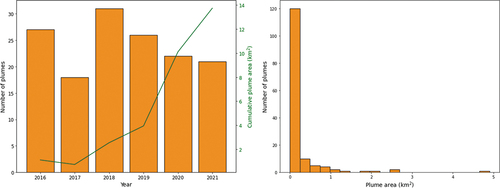
Table 2. Summary of imagery and plume statistics for each year of the study period.

	2016	2017	2018	2019	2020	2021
Sentinel-2 images examined in each season (n)	56	45	51	57	47	71
Sentinel-2 images with visible plumes (n)	14	8	15	14	13	14
Digitized plumes (n)	27	18	31	28	21	21
Average plume surface area (km^2) (1 S.D.)	0.04 (0.05)	0.04 (0.05)	0.08 (0.14)	0.14 (0.23)	0.48 (1.02)	0.66 (0.73)
Largest plume surface area (km^2)	0.19	0.22	0.74	0.94	4.17	2.60
Plume area error estimation range (km^2)	0.002–0.022	0.002–0.025	0.002–0.062	0.002–0.075	0.002–0.267	0.002–0.176

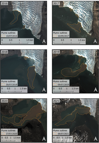
The majority of plumes identified at Blomstrandbreen are small in size (<1 km²) with most having surface areas of less than 0.25 km². However, the surface area of some plumes exceeded 2 km² (Table 2; Figure 2b), with the largest plume in the dataset observed on NaN Invalid Date with an area of 4.17 km² (±0.27 km²). This plume is substantially larger than any other plume mapped during the study. It was 1.50 km² larger than the next measured by the study, also in 2020 (26^th July) and 1.57 km² greater than the largest plume measured in 2021 (6^th July), which had a total surface area of 2.60 km² (±0.17 km²) (Figure 3).

Figure 3. Sentinel-2 images showing the largest sediment-laden meltwater plumes delineated in each year of the study period (2016 – 2021), including an example with the outlines of the plumes delineated in the 2016 image. Dates for each year are as follows, with the Julian day, (DOY) in brackets: 10/07/2016 (192), 10/09/2017 (253), 30/07/2018 (211), 09/07/2019 (190), 27/07/2020 (209), 06/07/2021 (187).

4.2. Supraglacial lake presence and variability

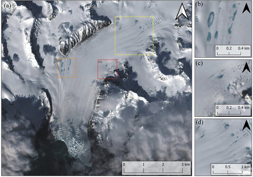
Analysis of cloud-free imagery of the upper ablation area of Blomstrandbreen shows the formation of SGLs on the surface of the glacier throughout the six-year study period. SGLs form in various locations across the glacier surface, but there are three areas in which they form most frequently (see Figure 4). In most cases, SGLs form in lateral foliations where two ice flow units meet, or in small hollow like depressions on the ice surface and regularly reform in these locations year after year.

Figure 4. (A) Sentinel-2 RGB image of the lower ablation area of Blomstrandbreen acquired on 14/06/2016, the three main areas where supraglacial lakes (SGLs) form are highlighted by boxes and are shown in panels (b), (c), and (d). (b) SGLs which form in longitudinal foliations created as a result of a tributary glacier flowing into the main branch of Blomstrandbreen. (c) Small SGLs on the eastern margin. (d) a swathe of SGLs which form in longitudinal foliations below the main crevasse field on Blomstrandbreen.

In most of the years within our study period, SGLs emerge in the first two weeks of June; although in the 2021 melt season there are no cloud free images until 3^rd July, and by this time there are numerous SGLs present on the surface of the glacier. This is the date with the greatest volume of surface water present throughout the study, equal to 5.28 × 10⁶ m³. In most other years, SGLs partially drain and refill at least once during the melt season, before draining in late August or in the early weeks of September. However, during the 2020 summer melt season, partial lake drainages occurred much earlier, between 23^rd and NaN Invalid Date NaNwith total surface water on the glacier reducing from 0.99 × 10⁶ m³ to 0.69 × 10⁶ m³ in this five day period. During the period between NaN Invalid Date NaNand NaN Invalid Date NaNof 2020 (there are no Sentinel-2 images within the < 20% cloud cover threshold), all SGLs on Blomstrandbreen had completely drained and did not refill again during the melt season. Comparatively, in 2021 there were three observable partial drainage events that took place during July between 3^rd and 6^th, 6^th and 17^th, and NaN Invalid Date NaNand 1^st August. The lakes refilled and compared to previous years, normal sized SGLs were present late into September with no evidence of drainage in the final image available to the study (NaN Invalid Date). Although SGLs can be observed on the glacier surface regularly during the study period, their area and subsequent volume are small in comparison with daily and seasonal runoff totals.

4.3. Glacial runoff and terminus position

Correlation coefficients (Pearson’s R value) show MAR-modelled glacial runoff has little to no influence on the surface area of plumes in 2016 and 2021 (Table 3). In the years including and between 2017 and 2020 there is a positive relationship between glacial runoff, this is the total runoff from up to two days prior to a plume surfacing, and plume surface area at Blomstrandbreen (r = 0.65–0.88, Table 3). The rate of terminus change in all years during the study period has little to no influence on plume area (r = −0.09–0.26).

Table 3. Correlation coefficient (Pearson r-value) between meltwater runoff and plume surface area, and rate of terminus change and plume surface area for each year.

	2016	2017	2018	2019	2020	2021
Meltwater runoff (mm water equivalent (w.e. d^−1))	0.08	0.84	0.74	0.88	0.65	0.05
Rate of terminus change (m/yr)	−0.09	0.26	0.12	−0.02	0.05	0.26

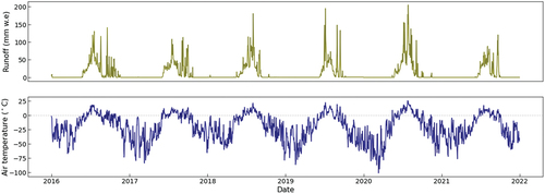
Glacial runoff on a single day exceeded 200 mm w.e. d⁻¹ in July 2020 and 150 mm w.e. d⁻¹ in 2018 and 2019 (Figure 5) which were three of the years that correlated most with plume surface area (Table 3). In 2018, the largest plume occurs prior to this peak in glacial runoff, whilst in 2019 the largest plume of that summer melt season surfaces three days after peak glacial runoff. In 2020 peak glacial runoff occurs the day after the largest plume in the study was identified, but followed multiple days with runoff >150 mm w.e. d⁻¹. In 2017, runoff marginally exceeded 100 mm w.e. d⁻¹ in a single day (113 and 108 mm w.e. d⁻¹ on 8^th September and 18^th July, respectively), these lower runoff values also result in a strongly positive relationship between runoff and plume area in this year, which correlates with the largest plume in this year (10^th September). Each year follows the same trend with the month of July having the highest runoff values and May the lowest. September has the greatest variation in runoff rates of any month, in some years, single days exceed 140 mm w.e. d⁻¹ (e.g. NaN Invalid Date) whilst in other years (2018) values are close to 0 mm w.e. d⁻¹ at the same point in the melt season.

Figure 5. Glacial runoff (mm w.E. d⁻¹) and air temperature (℃) at Blomstrandbreen modelled using MAR between 2016 – 2021.

4.4. Subglacial water routing

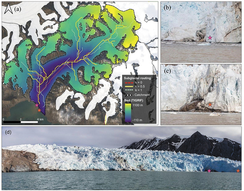
We undertook subglacial water routing to infer the location of subglacial channels beneath Blomstrandbreen and better understand where plumes may surface across the glacier front. We use the values of 0, 0.5 and 1 for k in Equation 5(5) $\mathrm{\Phi }={\rho }_{w}g\hspace{0.17em}Z+k\hspace{0.17em}{\rho }_{i}H$(5) , and identify potential subglacial pathways beneath Blomstrandbreen (Figure 6). The channels identified using k = 0 and k = 0.5 indicate a main channelized system that is likely present within the centralized region of the ~ 2.5–3.0 km wide glacier terminus (77 m difference between modelled locations), with k = 1 identifying a hydraulic potential pathway further east that may be present under high basal water pressures, 523 and 597 m from the other modelled channels, respectively. One possible reason for k = 1 routing subglacial flow to a more easterly location is the presence of an overdeepening at the bed of the glacier not far from the ice front (Lindbäck et al., 2018b). In addition to this, large bedrock bumps were visible beneath the glacier terminus of Blomstrandbreen close to the margin with the fjord during fieldwork in 2021, suggesting that water under high basal pressure may have been routed through the overdeepening and around these large bedrock obstacles to a more favourable location for evacuation (Figure 6). In spite of the alternative constant values (k), all of the preferred subglacial channels terminate in close proximity to where plumes are observed on the fjord surface throughout the six-year study period (see Figures 3 and 6).

Figure 6. (A) Potential subglacial channel routing beneath Blomstrandbreen using TIGRIF, overlaying a Sentinel-2 RGB image from 27/08/2021, with sediment-laden meltwater plume visible. Overlaid are indicative subglacial channels for k = 0.0, k = 0.5 and k = 1.0. Markers denote the location of a major outlet in 2021 and large bedrock bumps beneath the glacier exposed as a result of recent retreat. (b) Photograph of one of the major channels evacuating sediment-laden water into the fjord from beneath Blomstrandbreen, highlighted by marker on panel (a). (c) Photograph of one of the large bedrock bumps visible beneath the glacier exposed by recent retreat, highlighted by marker on panel (a). (d) Panorama of the western (left) and central (right) portions of the Blomstrandbreen margin, showing sections of ice above the grounding line and exposed bedrock beneath (left) and a separate flow section that remains marine-terminating (far right of image). The markers in panel (a) denote where close ups of the major channel (b) and the bedrock bumps (c) were taken. All photographs in (b), (c) and (d) were taken on 05/07/2021 during fieldwork at Blomstrandbreen.

5. Discussion

5.1. Controls on plume activity

We observe a significant increase in sediment-laden meltwater plume area at Blomstrandbreen between 2016 and 2021, however the frequency of plumes per season remains consistent (Table 2; Figure 2). These findings reveal glacial runoff is primarily responsible for the observed increases in plume magnitude with the rate of terminus change having little to no impact despite the retreat event that occurred between 2017 and 2018 (Figure 1). The total volume of glacial runoff does not fluctuate substantially in each season of the study period, but overall glacial runoff exerts the greatest control on plume size (see Table 3). This is due to large melt events which occur at various times across the study period, and can be highlighted by an event which takes place in late July 2020 when runoff reaches in excess of 200 mm w.e. d⁻¹. These high glacial runoff values correspond with large plume area measurements, up to 4.17 km² during this period (Figure 3).

High runoff rates during the melt season at Blomstrandbreen result in the configuration of an efficient hydrological system, as shown by the modelled output of the subglacial routing (Figure 6), allowing plumes to surface more readily. This is demonstrated by extremely high runoff rates (204 mm w.e. d-1) in July 2020 (Figure 4), when large plume surface areas were observed. It is noteworthy, however, that runoff totals in 2020 are much higher (5871.9 mm w.e. d-1) as a result of a large melt event early in July. This resulted in the surface area of plumes reducing rapidly thereafter, which suggests that the volume of meltwater evacuated earlier in the melt season may have exhausted the sources of sediment at the glacier ice-bed interface. Consequently, smaller plumes were formed later in the melt season. The larger volume of freshwater being discharged to Kongsfjorden early in the melt season may also result in fjord stratification, inhibiting the surfacing of plumes (e.g. De Andrés et al. 2020). This suggests that, as air temperatures increase and melt seasons lengthen, greater volumes of freshwater reaching fjord and coastal environments may impact upon the appearance of plumes in future years.

The eastern sector of the glacier front noticeably retreats after 2017, the result of this change is that the majority of plumes begin surfacing where the terminus was previously situated (see inset in Figure 1). In spite of this retreat, glacial runoff continues to be the greatest control on plume surface area, with the rate of terminus change having little-to-no influence on plume area (Table 3). However, we propose that the retreat of the glacier terminus between 2017 and 2018 may have impacted upon the magnitude of plumes; in 2016 and 2017 plumes mapped were mostly small in size (maximum plume area 0.22 km², mean plume area 0.04 km²), but when the ice front changed in the years after the retreat (2018–2021), they increased considerably (mean plume area, 0.3 km²) and upwelled in the notch that formed as a result of the altered terminus geometry. This is likely a result of an overdeepening, highlighted by subglacial DEMs (Lindbäck et al., 2018b) which the glacier was occupying in the first two years of the study storing sediment-laden water, and only releasing the suspended sediments in small volumes, when discharge was great enough to overcome the angle of the adverse bed slope. After 2018 when the glacier had retreated, the area in which sediment-laden water had been stored by the overdeepening was exposed. It is possible the terminus retreated into shallower water, enabling weaker plumes to reach the surface. Alternatively, runoff of similar intensity could produce larger plumes, given that any turbid meltwater evacuated from the glacier’s subglacial system into the fjord would no longer need to flow up an adverse bed slope.

On average, plume surface areas at Blomstrandbreen are smaller than those measured by How et al. (2017) at Kronebreen, situated in the same fjord complex. The differences in glacier catchments likely play a role in plume surface area, given that Kronebreen drains an ice area of ~295 km² compared to Blomstrandbreen which drains an ice area of ~80 km². Kronebreen is also the fastest flowing non-surging glacier on Svalbard, with velocities at the glacier’s tongue in winter reaching up to 1.5–2.0 m d⁻¹ and in summer peaking between 3.0–4.0 m d⁻¹ (Kääb, Lefauconnier, and Melvold 2005; Luckman et al. 2015). Blomstrandbreen and Kronebreen have very different bedrock topography, which may impact upon their meltwater and sediment outputs. Blomstrandbreen has a slightly inclined bed, with the last ~2 km of ice flowing downhill into Kongsfjorden, compared to Kronebreen which generally flows at a more consistent gradient from its upper reaches (Lindbäck et al., 2018b). Although the average plume surface area measured by this study was lower comparably to How et al. (2017) who used timelapse cameras stationed above the glacier front, the largest plumes at Blomstrandbreen were far larger than those measured at Kronebreen. We propose that this is a result of increasing air temperatures, resulting in higher melt rates in the intervening period between the field study at Kronebreen which was undertaken in the summer of 2014 and our remote sensing study which encompasses plume activity between 2016–2021.

It should be noted that plumes are a dynamic phenomena, surfacing and residing in fjords for minutes or hours and even possibly days. Consequently, data coverage provided by Sentinel-2 has some large gaps between image acquisition with visible plumes e.g. NaN Invalid Date and NaN Invalid Date . Some image data may also be removed because of the cloud cover filter (<20% per image) applied and therefore not all plumes at the ice front may have been identified throughout each of the six summer melt seasons.

5.2. Supraglacial lakes and their possible influence on plume activity

The timing, location, size, and duration of plumes are largely driven by hydrologic outputs and the efficiency of the subglacial hydrological system, reflecting variations in surface melt and runoff, as well as the potential implications of SGL drainage events. At Blomstrandbreen, SGLs are frequently observed in the upper ablation area throughout the melt seasons of 2016 to 2021, forming, draining and often refilling as each melt season progresses. Through analysis of available cloud-free imagery, our study has found evidence of SGLs draining, sometimes simultaneously preceding the surfacing of plumes at the glacier terminus (see Table 4). We suggest that the drainage of SGLs may have some influence on the emergence of plumes, as seen at Kronebreen, a larger glacier in the Kongsfjorden complex, where SGL drainages activated main meltwater plumes in its northern region (How et al. 2017).

Table 4. Examples of potential supraglacial lake drainages (partial or full) that may link to plume activity throughout the study period. A range is provided for potential drainages and when drainages may impact upon plumes, in most cases, due to the gaps in the availability of cloud-free satellite images. Dates are provided as Julian days (DOY).

	Potential period of SGL drainage	Visible plume activity in period after potential drainages
2016	184–187	187, 190
2017	214–242	242, 253
2018	187–196	196–197
2019	185–188	188, 190
2020	182–208	208, 209, 213
2021	198–213	213, 214, 215, 220

As SGLs drain, there is the potential for basal water pressure to increase and the subglacial system to become overwhelmed, which may not only impact localized ice velocity, but also impact the hydrologic configuration of the subglacial system, typically relating to distributed linked cavities or ‘inefficient drainage’ (Iken and Truffe 1997; Kamb 1987; Scholzen, Schuler, and Gilbert 2021). As modelled in Figure 6 under k = 1, increased basal water pressure may favour water accumulation and flow routing towards the eastern margin of the Blomstrandbreen terminus, where large plumes in excess of 2 km² were observed towards the end of July and beginning of August preceding SGL drainage events in the years 2020 and 2021.

Despite seeing a pattern of SGLs draining prior to plumes forming on the surface of the fjord in some years, a number of our observations suggest that plume surfacing is not strictly reliant upon the drainage of SGLs at other times during the six-year study period. For example, in 2020, all SGLs in the upper ablation area of Blomstrandbreen had drained by the end of July and did not refill during the remainder of the melt season. This was in spite of large plumes (>1.0 km²) surfacing throughout the middle of August and smaller plumes (<0.2 km²) being visible in the final week of the month even as runoff rates started to decline, demonstrating that glacier runoff is key to controlling plume area (Figure 5).

We find that there is no obvious relationship between plume surfacing and SGL drainage, despite both events occurring in parallel during periods of the melt season (Table 4). Visual quantification of the shape of SGLs, their surface area and volume at Blomstrandbreen suggest that SGL drainage may play a small role in plume upwelling, when considering the glacier volume and the proportion of SGL volume compared with annual runoff rates. However, should these drainages of small volumes occur rapidly, the hydrological system could become overwhelmed, in turn modifying the subglacial hydrology (e.g.Bartholomew et al. 2011). The initiation of these changes could mean that previously undisturbed sediment at the ice-bed interface may be suspended and flushed out, before being connected to more efficient areas of the hydrological system for discharge, resulting in a larger or new plume forming (e.g.Chu et al. 2009).

Many of the SGLs present on the surface of the glacier form in the same locations year-on-year, this points to some level of structural control on SGL area and therefore volume. Longitudinal foliations appear to be the main control on SGLs and are visible in the satellite imagery (Figure 4), these features occur when two flow units often of differing velocities meet (King et al. 2016). This is evident on the western margin of Blomstrandbreen where a small tributary glacier flows down from the north west into the main glacier branch, resulting in a number of SGLs forming in close proximity. Due to the structure of the longitudinal foliations, and the small, shallow hollows they create, it is quite likely that any SGLs that form in-situ will have relatively low water volumes because of the limiting ice surface topography. The position of SGLs has also been shown to be controlled by underlying bedrock topography (e.g. Turton et al. 2021). It is plausible that there are both surface and subsurface controls on the location of SGLs on Blomstrandbreen. On the eastern margin of the glacier, smaller features more akin to melt ponds form, however their surface areas are generally <0.01 km² which translates to a volume of ~ 0.027 × 10⁶ m³, we propose they are only likely to impact plume surfacing should they drain rapidly later in the season when the hydrological system is more efficient.

5.3. Recommendations for future research

Our research has shown the feasibility of manually delineating sediment-laden meltwater plumes at a marine-terminating glacier in Svalbard, and found that complex relationships between runoff, terminus position and glacier hydrology impact their surfacing in fjord waters. The study used optical imagery (Sentinel-2) covering the summer months (May to October), maximizing cloud-free imagery, but also coinciding with peak plume surfacing. As a result of using optical imagery, there were large gaps in our data coverage. We suggest utilizing a combination of high return frequency satellites, this may be a combination of active radar, which can see through cloud, and additional passive sensors, for example those from Planet Labs, with higher temporal and spatial resolution to better understand the dynamic processes occurring at glacier fronts.

Future research should focus on a greater number of marine-terminating glacier locations across the Svalbard archipelago. GEEDiT (Lea 2018) could be used for this, as it is a powerful tool in which to undertake rapid manual delineations, scalable across multiple locations. However, a method could be devised to automatically delineate plumes using remote sensing datasets, for example in Google Earth Engine due to its cloud computing nature and rapid data processing capabilities, and to quantify the difference between sediment-laden meltwater plume surfacing and calving events using higher temporal resolution Synthetic Aperture Radar data at a much greater spatial scale e.g. Svalbard-wide. Additional research could utilize empirically derived area-to-volume converters to provide insights into SGL dynamics which may contribute to better understanding of the influence of runoff, glacier retreat and subglacial hydrology on the surfacing of plumes. In-situ empirical data collected at glacier calving fronts such as conductivity, temperature, and depth profiles can act as ground truthing, assisting with future remote sensing studies of similar locations. This data can also be utilized in modelling studies for locations where it is not possible to collect in-situ measurements, and be combined with automated thresholding using optical imagery to better determine the volumes of sediment not only at the surface, but also at depth.

6. Conclusions

The surfacing of sediment-laden meltwater plumes at Blomstrandbreen reflects the wider relationship between glacial runoff, subglacial routing of meltwater and the glacier’s terminus position. We find that plume surfacing at Blomstrandbreen remains stable throughout the six-year study period, but the size of plumes which surface increases significantly in 2020 and 2021, corresponding with increasing glacial runoff and a larger number of supraglacial lakes forming in the glacier’s upper ablation area. Our findings suggest there is little correlation between the rate of glacier terminus change and the emergence of surfacing plumes at Blomstrandbreen, but that a retreat event between 2017 – 2018 May have impacted upon plume magnitude, allowing for greater volumes of suspended sediments to reach the fjord surface. We therefore suggest more research is needed across the archipelago of Svalbard to derive a direct relationship between glacier retreat and sediment-laden meltwater plume surfacing as a result of our findings at Blomstrandbreen.

Acknowledgements

The authors would like to thank James Lea for the design and updates to the GEEDiT tool which made various aspects of this work possible. We would also like to thank Xavier Fettweis for providing regional climate model MAR data, and ESA’s Copernicus Open Access Hub for use of Sentinel-2 imagery. We are grateful to the Norwegian Polar Data Centre for access to the Tidewater Glacier Retreat Impact on Fjord Circulation and Ecosystems digital bed elevation model (see Lindbäck et al., 2018a) used in calculating subglacial pathways. The authors would like to thank Jonathan Slessor for the photographs he provided to be used in this paper.

Disclosure statement

No potential conflict of interest was reported by the authors.

Data Availability statement

Terminus, plume and supraglacial lake outlines that support the key findings of this study are available from the corresponding author, [G.D.T], upon request. Regional climate model MAR v3.11.5 data was provided by Dr Xavier Fettweis and is freely available via ftp.climato.be/fettweis. Ice velocity data used in this study are openly available at Service de données de l’Observatoire Midi-Pyrénées at https://doi.org/10.6096/1007.

Additional information

Funding

This work was supported by Natural Environment Research Council PhD studentships awarded to G.D.T., and L.D.R: [NE/L002493/1], and [NE/L002450/1], respectively. C.J.S. receives funding through a Natural Environment Research Council Standard Grant [NE/X000435/1]. G.D.T was also supported by a SIOS Research Infrastructure Access project in 2021 through the Research Council of Norway, project number 291644, Svalbard Integrated Arctic Earth Observing System – Knowledge Centre, operational phase.

References

- Bartholomew, I., P. Nienow, A. Sole, D. Mair, T. Cowton, S. Palmer, and J. Wadham. 2011. “Supraglacial Forcing of Subglacial Drainage in the Ablation Zone of the Greenland Ice Sheet.” Geophysical Research Letters 38 (8): L08502. https://doi.org/10.1029/2011GL047063.
- Beason, S. R. 2017. “Change in Glacial Extent at Mount Rainier National Park from 1896 to 2015.” Natural Resource Report. NPS/MORA/NRR—2017/1472. Fort Collins, Colorado: National Park Service.
- Box, J. E., W. T. Colgan, B. Wouters, D. O. Burgess, S. O’Neel, L. I. Thomson, and S. H. Mernild. 2018. “Global Sea-Level Contribution from Arctic Land Ice: 1971–2017.” Environmental Research Letters 13 (12): 125012. https://doi.org/10.1088/1748-9326/aaf2ed.
- Burton, D. J., J. A. Dowdeswell, K. A. Hogan, and R. Noormets. 2016. “Marginal Fluctuations of a Svalbard Surge-Type Tidewater Glacier, Blomstrandbreen, Since the Little Ice Age: A Record of Three Surges.” Arctic, Antarctic, and Alpine Research 48 (2): 411–426. https://doi.org/10.1657/AAAR0014-094.
- Carisio, S. P. 2012. “Evaluating areal errors in Northern Cascade Glacier inventories.” M.S. Geography Thesis, University of Delaware. http://udspace.udel.edu/handle/19716/12643.
- Carroll, D., D. A. Sutherland, B. Hudson, T. Moon, G. A. Catania, E. L. Shroyer, J. D. Nash, et al. 2016. “The Impact of Glacier Geometry on Meltwater Plume Structure and Submarine Melt in Greenland Fjords.” Geophysical Research Letters 43 (18): 9739–9748. https://doi.org/10.1002/2016GL070170.
- Carr, J. R., C. R. Stokes, and A. Vieli. 2013. “Recent Progress in Understanding Marine-Terminating Arctic Outlet Glacier Response to Climatic and Oceanic Forcing: Twenty Years of Rapid Change.” Progress in Physical Geography 37 (4): 436–467. https://doi.org/10.1177/0309133313483163.
- Chu, V. W., L. C. Smith, A. K. Rennermalm, R. R. Forster, and J. E. Box. 2012. “Hydrologic Controls on Coastal Suspended Sediment Plumes Around the Greenland Ice Sheet.” The Cryosphere 6 (1): 1–19. https://doi.org/10.5194/tc-6-1-2012.
- Chu, V. W., L. C. Smith, A. K. Rennermalm, R. R. Forster, J. E. Box, and N. Reeh. 2009. “Sediment Plume Response to Surface Melting and Supraglacial Lake Drainages on the Greenland Ice Sheet.” Journal of Glaciology 55 (194): 1072–1082. https://doi.org/10.3189/002214309790794904.
- Cook, S. J., and D. J. Quincey. 2015. “Estimating the Volume of Alpine Glacial Lakes.” Earth Surface Dynamics 3 (4): 559–575. https://doi.org/10.5194/esurf-3-559-2015.
- Darlington, E. F. 2015. “Meltwater delivery from the tidewater glacier Kronebreen to Kongsfjorden, Svalbard; insights from in-situ and remote-sensing analyses of sediment plumes.” PhD thesis, Loughborough University. https://hdl.handle.net/2134/19399.
- De Andrés, E., D. A. Slater, F. Straneo, J. Otero, S. Das, and F. Navarro. 2020. “Surface Emergence of Glacial Plumes Determined by Fjord Stratification.” The Cryosphere 14 (6): 1951–1969. https://doi.org/10.5194/tc-14-1951-2020.
- Decaux, L., M. Grabiec, D. Ignatiuk, and J. Jania. 2019. “Role of Discrete Water Recharge from Supraglacial Drainage Systems in Modeling Patterns of Subglacial Conduits in Svalbard Glaciers.” The Cryosphere 13 (3): 735–752. https://doi.org/10.5194/tc-13-735-2019.
- Dowdeswell, J. A., K. A. Hogan, N. S. Arnold, R. I. Mugford, M. Wells, J. P. P. Hirst, and C. Decalf. 2015. “Sediment‐Rich Meltwater Plumes and Ice‐Proximal Fans at the Margins of Modern and Ancient Tidewater Glaciers: Observations and Modelling.” Sedimentology 62 (6): 1665–1692. https://doi.org/10.1111/sed.12198.
- Everett, A., J. Kohler, A. Sundfjord, K. M. Kovacs, T. Torsvik, A. Pramanik, L. Boehme, and C. Lydersen. 2018. “Subglacial Discharge Plume Behaviour Revealed by CTD-Instrumented Ringed Seals.” Scientific Reports 8 (1): 1–10. https://doi.org/10.1038/s41598-018-31875-8.
- Fried, M. J., Catania, G. A., Bartholomaus, T. C., Duncan, D., Davis, M., Stearns, L. A., Nash, J., Shroyer, E and D. Sutherland. 2015. “Distributed subglacial discharge drives significant submarine melt at a Greenland tidewater glacier.“ Geophysical Research Letters 42 (21): 9328–9336. https://doi.org/10.1002/2015GL065806.
- Hagen, J. O., O. Liestøl, E. R. I. K. Roland, and T. Jørgensen. 1993. Glacier Atlas of Svalbard and Jan Mayen, 129. Oslo: Norsk Polarinstitutt Meddelelser. http://hdl.handle.net/11250/173065.
- Hewitt, I. J. 2020. “Subglacial Plumes.” Annual Review of Fluid Mechanics 52 (1): 145–169. https://doi.org/10.1146/annurev-fluid-010719-060252.
- Hodgkins, R., R. Bryant, E. Darlington, and M. Brandon. 2016. “Pre-Melt-Season Sediment Plume Variability at Jökulsárlón, Iceland, a Preliminary Evaluation Using in-Situ Spectroradiometry and Satellite Imagery.” Annals of Glaciology 57 (73): 39–46. https://doi.org/10.1017/aog.2016.20.
- Hopwood, M. J., D. Carroll, T. Dunse, A. Hodson, J. M. Holding, J. L. Iriarte, S. Ribeiro, et al. 2020. “How Does Glacier Discharge Affect Marine Biogeochemistry and Primary Production in the Arctic?” The Cryosphere 14 (4): 1347–1383. https://doi.org/10.5194/tc-14-1347-2020.
- How, P., D. I. Benn, N. R. Hulton, B. Hubbard, A. Luckman, H. Sevestre, W. J. Van Pelt, K. Lindbäck, J. Kohler, and W. Boot. 2017. “Rapidly Changing Subglacial Hydrological Pathways at a Tidewater Glacier Revealed Through Simultaneous Observations of Water Pressure, Supraglacial Lakes, Meltwater Plumes and Surface Velocities.” The Cryosphere 11 (6): 2691–2710. https://doi.org/10.5194/tc-11-2691-2017.
- Hudson, B., I. Overeem, D. McGrath, J. P. M. Syvitski, A. Mikkelsen, and B. Hasholt. 2014. “MODIS Observed Increase in Duration and Spatial Extent of Sediment Plumes in Greenland Fjords.” The Cryosphere 8 (4): 1161–1176. https://doi.org/10.5194/tc-8-1161-2014.
- Iken, A., and M. Truffe. 1997. “The Relationship Between Subglacial Water Pressure and Velocity of Findelengletscher, Switzerland, During Its Advance and Retreat.” Journal of Glaciology 43 (144): 328–338. https://doi.org/10.3189/S0022143000003282.
- Kääb, A., B. Lefauconnier, and K. Melvold. 2005. “Flow Field of Kronebreen, Svalbard, Using Repeated Landsat 7 and ASTER Data.” Annals of Glaciology 42:7–13. https://doi.org/10.3189/172756405781812916.
- Kamb, B. 1987. “Glacier Surge Mechanism Based on Linked Cavity Configuration of the Basal Water Conduit System.” Journal of Geophysical Research: Solid Earth 92 (B9): 9083–9100. https://doi.org/10.1029/JB092iB09p09083.
- Kehrl, L. M., R. L. Hawley, R. D. Powell, and J. Brigham-Grette. 2011. “Glacimarine Sedimentation Processes at Kronebreen and Kongsvegen, Svalbard.” Journal of Glaciology 57 (205): 841–847. https://doi.org/10.3189/002214311798043708.
- King, O., M. J. Hambrey, T. D. Irvine‐Fynn, and T. O. Holt. 2016. “The Structural, Geometric and Volumetric Changes of a Polythermal Arctic Glacier During a Surge Cycle: Comfortlessbreen, Svalbard.” Earth Surface Processes and Landforms 41 (2): 162–177. https://doi.org/10.1002/esp.3796.
- Lea, J. M. 2018. “The Google Earth Engine Digitisation Tool (GEEDiT) and the Margin Change Quantification Tool (MaQit)–Simple Tools for the Rapid Mapping and Quantification of Changing Earth Surface Margins.” Earth Surface Dynamics 6 (3): 551–561. https://doi.org/10.5194/esurf-6-551-2018.
- Lindbäck, K., J. Kohler, R. Pettersson, C. Nuth, K. Langley, A. Messerli, D. Vallot, K. Matsuoka, and O. Brandt. 2018a. Subglacial Topography, Ice Thickness, and Bathymetry of Kongsfjorden, Northwestern Svalbard [Data Set]. Norwegian Polar Institute. https://doi.org/10.21334/npolar.2017.702ca4a7.
- Lindbäck, K., J. Kohler, R. Pettersson, C. Nuth, K. Langley, A. Messerli, D. Vallot, K. Matsuoka, and O. Brandt. 2018b. “Subglacial Topography, Ice Thickness, and Bathymetry of Kongsfjorden, Northwestern Svalbard.” Earth System Science Data 10 (4): 1769–1781. https://doi.org/10.5194/essd-10-1769-2018.
- Luckman, A., D. I. Benn, F. Cottier, S. Bevan, F. Nilsen, and M. Inall. 2015. “Calving Rates at Tidewater Glaciers Vary Strongly with Ocean Temperature.” Nature Communications 6 (1): 1–7. https://doi.org/10.1038/ncomms9566.
- Lydersen, C., P. Assmy, S. Falk-Petersen, J. Kohler, K. M. Kovacs, M. Reigstad, H. Steen, et al. 2014. “The Importance of Tidewater Glaciers for Marine Mammals and Seabirds in Svalbard, Norway.” Journal of Marine Systems 129:452–471. https://doi.org/10.1016/j.jmarsys.2013.09.006.
- Mansell, D., A. Luckman, and T. Murray. 2012. “Dynamics of Tidewater Surge-Type Glaciers in Northwest Svalbard.” Journal of Glaciology 58 (207): 110–118. https://doi.org/10.3189/2012JoG11J058.
- Marshall, G. J., J. A. Dowdeswell, and W. G. Rees. 1994. “The Spatial and Temporal Effect of Cloud Cover on the Acquisition of High Quality Landsat Imagery in the European Arctic Sector.” Remote Sensing of Environment 50 (2): 149–160. https://doi.org/10.1016/0034-42579490041-8.
- Marshall, G. J., W. G. Rees, and J. A. Dowdeswell. 1993. “Limitations Imposed by Cloud Cover on Multitemporal Visible Band Satellite Data Sets from Polar Regions.” Annals of Glaciology 17:113–120. https://doi.org/10.3189/S0260305500012696.
- McGrath, D., K. Steffen, I. Overeem, S. H. Mernild, B. Hasholt, and M. Van Den Broeke. 2010. “Sediment Plumes as a Proxy for Local Ice-Sheet Runoff in Kangerlussuaq Fjord, West Greenland.” Journal of Glaciology 56 (199): 813–821. https://doi.org/10.3189/002214310794457227.
- Meslard, F., F. Bourrin, G. Many, and P. Kerhervé. 2018. “Suspended Particle Dynamics and Fluxes in an Arctic Fjord (Kongsfjorden, Svalbard).” Estuarine, Coastal and Shelf Science 204:212–224. https://doi.org/10.1016/j.ecss.2018.02.020.
- Millan, R., J. Mouginot, A. Rabatel, and M. Morlighem. 2022. “Ice Velocity and Thickness of the World’s Glaciers.” Nature Geoscience 15 (2): 124–129. https://doi.org/10.1038/s41561-021-00885-z.
- Mugford, R. I., and J. A. Dowdeswell. 2011. “Modeling Glacial Meltwater Plume Dynamics and Sedimentation in High‐Latitude Fjords.” Journal of Geophysical Research: Earth Surface 116 (F1): F1. https://doi.org/10.1029/2010JF001735.
- Nanni, U., F. Gimbert, P. Roux, and A. Lecointre. 2021. “Observing the Subglacial Hydrology Network and Its Dynamics with a Dense Seismic Array.” Proceedings of the National Academy of Sciences 118 (28). https://doi.org/10.1073/pnas.2023757118.
- O’Callaghan, J. F., and D. M. Mark. 1984. “The Extraction of Drainage Networks from Digital Elevation Data.” Computer Vision, Graphics and Image Processing 28 (3): 323–344. https://doi.org/10.1016/S0734-189X(84)80011-0.
- Østby, T. I., T. V. Schuler, and S. Westermann. 2014. “Severe Cloud Contamination of MODIS Land Surface Temperatures Over an Arctic Ice Cap, Svalbard.” Remote Sensing of Environment 142:95–102. https://doi.org/10.1016/j.rse.2013.11.005.
- Schild, K. M., R. L. Hawley, J. W. Chipman, and D. I. Benn. 2017. “Quantifying Suspended Sediment Concentration in Subglacial Sediment Plumes Discharging from Two Svalbard Tidewater Glaciers Using Landsat-8 and in situ Measurements.” International Journal of Remote Sensing 38 (23): 6865–6881. https://doi.org/10.1080/01431161.2017.1365388.
- Schild, K. M., C. E. Renshaw, D. I. Benn, A. Luckman, R. L. Hawley, P. How, L. Trusel, F. R. Cottier, A. Pramanik, and N. R. J. Hulton. 2018. “Glacier Calving Rates Due to Subglacial Discharge, Fjord Circulation, and Free Convection.” Journal of Geophysical Research: Earth Surface 123 (9): 2189–2204. https://doi.org/10.1029/2017JF004520.
- Scholzen, C., T. V. Schuler, and A. Gilbert. 2021. “Sensitivity of Subglacial Drainage to Water Supply Distribution at the Kongsfjord Basin, Svalbard.” The Cryosphere 15 (6): 2719–2738. https://doi.org/10.5194/tc-15-2719-2021.
- Sevestre, H., and D. I. Benn. 2015. “Climatic and Geometric Controls on the Global Distribution of Surge-Type Glaciers: Implications for a Unifying Model of Surging.” Journal of Glaciology 61 (228): 646–662. https://doi.org/10.3189/2015JoG14J136.
- Shreve, R. L. 1972. “Movement of Water in Glaciers.” Journal of Glaciology 11 (62): 205–214. https://doi.org/10.3189/S002214300002219X.
- Slater, D., P. Nienow, A. Sole, T. Cowton, R. Mottram, P. Langen, and D. Mair. 2017. “Spatially Distributed Runoff at the Grounding Line of a Large Greenlandic Tidewater Glacier Inferred from Plume Modelling.” Journal of Glaciology 63 (238): 309–323. https://doi.org/10.1017/jog.2016.139.
- Sund, M., and T. Eiken. 2010. “Recent Surges on Blomstrandbreen, Comfortlessbreen and Nathorstbreen, Svalbard.” Journal of Glaciology 56 (195): 182–184. https://doi.org/10.3189/002214310791190910.
- Tallentire, G. D., J. Evans, R. Hodgkins, and E. F. Darlington. 2022. “Quantifying SSC Variability in Sediment-Laden Meltwater Plumes Using in-Situ Data and Simulated Satellite Remote Sensing Bandwidths.” Authorea Preprints. https://doi.org/10.1002/essoar.10512520.1.
- Tedstone, A. J., and N. S. Arnold. 2012. “Automated Remote Sensing of Sediment Plumes for Identification of Runoff from the Greenland Ice Sheet.” Journal of Glaciology 58 (210): 699–712. https://doi.org/10.3189/2012JoG11J204.
- Torsvik, T., Albretsen, J., Sundfjord, A., Kohler, J. Sandvik. A. Dagrun, Skarðhamar, J., Lindbäck, K. and A. Everett. 2019. “Impact of tidewater glacier retreat on the fjord system: Modeling present and future circulation in Kongsfjorden, Svalbard.“ Estuarine, Coastal and Shelf Science 220: 152–165. https://doi.org/10.1016/j.ecss.2019.02.005.
- Trusel, L. D., Powell, R. D., Cumpston, R. M, and J. Brigham-Grette. 2010. “Modern glacimarine processes and potential future behaviour of Kronebreen and Kongsvegen polythermal tidewater glaciers, Kongsfjorden, Svalbard.“ SP 344 (1): 89–102. https://doi.org/10.1144/SP344.9.
- Turton, J. V., P. Hochreuther, N. Reimann, and M. T. Blau. 2021. “The Distribution and Evolution of Supraglacial Lakes on 79° N Glacier (North-Eastern Greenland) and Interannual Climatic Controls.” The Cryosphere 15 (8): 3877–3896. https://doi.org/10.5194/tc-15-3877-2021.
- van as, D., B. Hasholt, A. P. Ahlstrøm, J. E. Box, J. Cappelen, W. Colgan, R. S. Fausto, et al. 2018. “Reconstructing Greenland Ice Sheet Meltwater Discharge Through the Watson River (1949–2017).” Arctic, Antarctic, and Alpine Research 50 (1): 1. https://doi.org/10.1080/15230430.2018.1433799.
- Wawrzyniak, T., and M. Osuch. 2020. “A 40-Year High Arctic Climatological Dataset of the Polish Polar Station Hornsund (SW Spitsbergen, Svalbard).” Earth System Science Data 12 (2): 805–815. https://doi.org/10.5194/essd-12-805-2020.