
ABSTRACT
Aboveground biomass (AGB) and leaf area index (LAI) are key variables of ecosystem processes and functioning. Knowledge is lacking on how well the seasonal patterns of ground vegetation AGB and LAI can be detected by satellite images in boreal ecosystems. We conducted field measurements between May and September during one growing season to investigate the seasonal development of ground vegetation AGB and LAI of seven plant functional types (PFTs) across seven vegetation types (VTs) within three peatland and forest study areas in northern Finland. We upscaled field-measured AGB and LAI with Sentinel-2 (S2) imagery by applying random forest (RF) regressions. Field-measured AGB peaked around the first week of August and, in most cases, one to two weeks later than LAI. Regarding PFTs, deciduous vascular plants had clear unimodal seasonal patterns, while the AGB and LAI of evergreen vegetation and mosses remained steady over the season. Remote sensing regression models explained 24.2–50.2% of the AGB (RMSE: 78.8–198.7 g m−2) and 48.5–56.1% of the LAI (RMSE: 0.207–0.497 m2 m−2) across sites. Peatland-dominant sites and VTs had a higher prediction accuracy. S2-predicted peak dates of AGB and LAI were one to three weeks earlier than the field-based ones. Our findings suggest that boreal ground vegetation seasonality varies among PFTs and VTs and that S2 time series data can be applied to monitor its spatiotemporal patterns, especially in treeless regions.
1. Introduction
The boreal ecosystem, mosaic of forests, peatlands, and waterbodies, covers about 10% of Earth’s land surface area at 50–70°N (Helbig et al. Citation2020). It is characterized by a cool climate with relatively low precipitation and serves as a significant reservoir for organic carbon, storing about 1,000 Gt carbon above and below ground, particularly within peatlands (Bradshaw and Warkentin Citation2015). The region is susceptible to environmental changes and is facing rapid climate warming (Helbig et al. Citation2020; Lyons et al. Citation2020; Mcpartland et al. Citation2020). Increasing air temperature has led to changes in vegetation phenology, which refers to the conjunctional seasonal trajectory of plant physiological activity, growth, biomass, and canopy coverage changes, consequently altering the carbon cycle within ecosystems (Mäkiranta et al. Citation2018; Richardson et al. Citation2013).
Two key plant traits, aboveground biomass (AGB), which is defined as the total quantity of aboveground dry mass and living and dead plant matter (g m−2) (Verwijst and Telenius Citation1999), and leaf area index (LAI), which estimates the one-sided green leaf area per unit of ground area (m2 m−2) (Chen and Black Citation1992), are generally known to regulate plant productivity and are hence valuable indicators for assessing the ecosystem carbon balance (Peichl et al. Citation2018; Tian, Branfireun, and Lindo Citation2020). The phenology patterns of these traits are responding to climatic changes, for example, an earlier spring onset boosts AGB accumulation (Koebsch et al. Citation2020) and a longer growing season causes seasonal increases in LAI (Zhu and Zeng Citation2017).
Ground vegetation (the component of the understory that is <1.5 m tall) forms a significant part of total vegetation AGB and LAI in boreal ecosystems (Macdonald et al. Citation2012). Due to the high spatial heterogeneity along with environmental gradients in the boreal biome, there are various ground vegetation community types (VTs) with differentiated plant functional type (PFT) composition (Korrensalo et al. Citation2018; Lyons et al. Citation2020; Pohjanmies et al. Citation2021; Räsänen et al. Citation2020). The PFTs, such as evergreen and deciduous shrubs, forbs, graminoids, and mosses, and consequently also VTs have divergent seasonal patterns in AGB and LAI. For instance, in peatlands, VTs can include elongated strings dominated by Ericaceous shrubs, lawns with sedges, forbs, and Sphagnum, and flarks covered by brown mosses and sedges (Laitinen et al. Citation2017; Peterka et al. Citation2017; Räsänen et al. Citation2020). As reported by Korrensalo et al. (Citation2018), the live-standing biomass within a growing season ranged from 211 g m−2 in bare peat surfaces without Sphagnum to 979 g m−2 in high hummock VTs. However, only few studies have reported comprehensive comparisons of how AGB and LAI vary at different scales, namely across landscapes, VTs, and PFTs.
There is an ever-growing trend in integrating remote sensing data with field measurements to enhance our understanding of vegetation patterns, both spatially and temporally, and facilitate accurate carbon balance estimations (Juutinen et al. Citation2017; Linkosalmi et al. Citation2022; Skidmore et al. Citation2021). The satellites with high spatial and temporal resolution, such as Sentinel-2 (S2), allow to estimate plant biological properties and further to capture their seasonal development across landscapes (e.g., (Juutinen et al. Citation2017; Pang et al. Citation2022; Puliti et al. Citation2020; Räsänen et al. Citation2021)). Previous research has shown that S2 performs better than the Landsat series for estimating AGB and LAI in the boreal biome (Astola et al. Citation2019; Korhonen, Packalen, and Rautiainen Citation2017; Majasalmi and Rautiainen Citation2016), providing plausible maps of these plant traits in boreal forests (Korhonen, Packalen, and Rautiainen Citation2017; Puliti et al. Citation2020) and peatlands (Arroyo-Mora et al. Citation2018; Czapiewski and Szuminska Citation2022; Räsänen et al. Citation2021).
Time-series S2 data has been utilized to track vegetation phenology (Descals et al. Citation2020; Misra, Cawkwell, and Wingler Citation2020; Schiefer et al. Citation2023; Thapa, Millan, and Eklundh Citation2021). For example, Linkosalmi et al. (Citation2022) combined S2 data with digital photography in boreal peatlands and Thapa, Millan, and Eklundh (Citation2021) assessed S2-based phenology in hemi boreal forests, and Tian et al. (Citation2021) estimated the performance S2-based phenology estimates with the help of Europe-wide in-situ observations. However, to the best of our knowledge, no studies have investigated the seasonal development of boreal ground vegetation AGB and LAI using S2 data and linked the S2-based AGB and LAI estimates to field-based PFT and VT-specific AGB and LAI estimates.
To address this gap, our objective is to monitor field layer AGB and LAI in different PFTs and VTs with the help of field inventory and S2 data in three boreal peatland-dominated ecosystems from May to October in 2017 or 2019. Our main emphasis is on treeless VTs. We ask the following questions: (1) what are the seasonal patterns of ground vegetation AGB and LAI, and how do these vary among VTs and PFTs, (2) can field measurements be upscaled regionally with S2 data, and (3) what are the spatiotemporal patterns of AGB and LAI at the landscape scale?
2. Study sites
We studied three peatland-dominated areas that are surrounded by forests in northern Finland (67°–69° N, ). The study sites, Pallas, Sodankylä, and Kaamanen, have different biological, geological, and topographical characteristics, allowing a good comparison among landscapes (Räsänen et al. Citation2020). The mean annual temperatures were 0.30°C, 0.03°C, and 0.02°C and the mean annual precipitations were 599 mm, 518 mm, and 455 mm in 2008–2019 at the three sites, respectively (Fig. S1). Within this reference period, the average accumulation of degree-days above 5°C (DD5) was approximately 1500 during the growing seasons (Fig. S1). The spatial vegetation characteristics of these sites have been previously reported in detail (Aurela et al. Citation2015; Lohila et al. Citation2015; Räsänen et al. Citation2020), but the seasonal development of AGB and LAI remain undocumented.
Figure 1. Locations and land cover classification maps of the study sites with landscape photos, in Pallas (a), Sodankylä (b), and Kaamanen (c) with analysis radii of 1500 m, 300 m, and 300 m, respectively; and the national background (d). The classification maps were produced by Räsänen and Virtanen (Citation2019) for Kaamanen, Räsänen et al. (Citation2021) for Pallas, and Mikola et al. (in prep.) for Sodankylä.
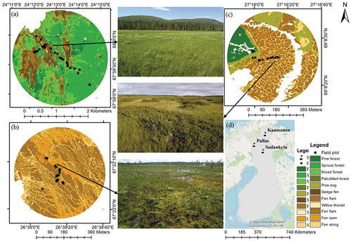
The Pallas site () consists of a rather open, nutrient-rich sedge fen-dominated peatland (Lompolojänkkä, 67°59.835′N, 24°12.546′E, 269 m a.s.l.) and a mixed, spruce-dominated forest (Kenttärova, 67°59.237’ N, 24°14.579’ E, 347 m a.s.l.). The peatland is characterized by four major VTs: pine bog, sedge fen, willow thicket, and flark fen (). The pine bog VT is located in the marginal area between the fen and the forest, covering dwarf shrubs (e.g. Vaccinium myrtillus, V. vitis-idaea, V. oxycoccos, and V. uliginosum), feather mosses (e.g. Pleurozium schreberi and Dicranum majus), and Sphagnum. The sedge fen is dominated by Carex rostrata and Sphagnum lindbergii; willow thickets (Salix phylicifolia and S. lapponum) approximately 60 cm in height line the narrow stream running through the fen; and wet flarks are covered in Carex spp. and brown mosses, especially Scorpidium scorpioides. The main tree species in the upland forest site Kenttärova is Norway spruce (Picea abies) mixed with deciduous trees e.g. Betula pubescens, Populus tremula, and Salix caprea. The field layer primarily consists of dwarf shrubs, and the ground layer is covered by feather mosses with occasional liverworts and lichens (Table S1; (Aurela et al. Citation2015; Lohila et al. Citation2015; Pearson et al. Citation2015)).
Table 1. Summary of vegetation inventories and Sentinel-2 image collections. Bolded dates indicate matched field-Sentinel-2 records.
The Halssiaapa site in Sodankylä (67°22.117’ N, 26°39.244’ E, 180 m a.s.l.) is a patterned fen with a shallow string – lawn–flark microtopography (). The narrow (0.5–1 m wide) and interconnected strings are covered by various shrubs, such as Betula nana, and flarks are dominated by wet brown mosses (esp. Sarmentypnum spp.) and sedges, and a few scattered small birches (Betula pubescens) and pine (Pinus sylvestris) are found in the strings. Lawns are covered by Sphagnum and forbs. Flooding water from melting snow inundates the low surfaces from May to early June and occasionally over the summer (Table S1; (Haapala et al. Citation2009; Mörsky et al. Citation2012)).
The Kaamanen site is a patterned fen (69°8.435’ N, 27°16.189 E, 155 m a.s.l., ) characterized by alternating strings and flarks. A pine forest (Pinus sylvestris) surrounds the fen. Pine bog VT is common on fen margins, covered by various ericaceous shrubs and forbs, and with a dense cover of feather mosses and Sphagnum. A stream runs through the fen from north to south. In the middle, dry strings are up to 1 m high and 5 m wide, their vegetation consisting of evergreen shrubs and forbs. Wet flarks with Carex spp. vegetation is influenced by periodical flooding. Intermediate habitats between strings and flarks are shrub-dominated (mostly Betula nana) with abundant Carex spp. and S. lindbergii carpets (Table S1; (Maanavilja et al. Citation2011; Räsänen and Virtanen Citation2019)).
3. Materials and methods
First, we measured the %-cover of plant species and the height of vascular plants to estimate the seasonal development of AGB and LAI in different VTs in the field. Second, we explored the field-measured vegetation seasonal patterns in terms of VTs and PFTs. Third, we upscaled field measurements with S2 time series images and random forest (RF) regressions (Breiman Citation2001) to assess spatiotemporal patterns of total ground vegetation AGB and LAI. Additionally, we compared the differences in field- and satellite-estimated vegetation patterns ().
Figure 2. Flowchart of the data acquisition and analysis processes. In the figure, S2 L2A refers to Sentinel 2 Level 2A product, 3D %-cover to three-dimensional %-cover, AGB to aboveground biomass, LAI to leaf area index, VTs to vegetation types, and PFTs to plant functional types.
3.1. Field inventories and vegetation data processing
We inventoried ground vegetation over a growing season, from May to October, in Kaamanen in 2017 and in Pallas and Sodankylä in 2019 ( and ). We sampled 84 (Pallas), 43 (Sodankylä), and 18 (Kaamanen) circular plots with a 50-cm diameter, representing the main local VTs (Fig. S2). We visited plots biweekly; and in total, we obtained 1147 inventory records (). During inventories, we aimed to identify the plant species but, in some cases, only the genera level was achieved (Table S1). We visually estimated the three-dimensional %-cover for each plant taxa (3D %-cover, since the ground and field layer were estimated separately, typically the sum of all taxa > 100%) (Figs. S3 and S4). We further divided the 3D %-cover into the green, photosynthesizing part and the brown, woody fraction. We measured the average height of each vascular plant species or genus with a ruler. Plot locations were measured with a Trimble R10 GPS device with a 5-cm accuracy.
We examined how a five-degree (>5°C) day temperature sum (DD5) development relates with AGB and LAI across sites and between years. For analyzing the vegetation data by specific growing periods, we categorized our field inventories into three temporal windows by DD5 developments, including early- (May to the first week of July, i.e. DD5 was ca. 600°C, at one-third of its highest level), mid- (mid-July to the first week of August, i.e. DD5 was ca. at half of its highest level), and late- (mid-August to October, i.e. DD5 approached its top level) seasons ( and Fig. S1).
We grouped the plant species and genera into seven PFTs: evergreen shrubs, deciduous shrubs, forbs, graminoids, brown mosses, feather mosses, and Sphagnum (Table S1). Lichens were lacking or were scarce in our study plots, so we omitted them from the analyses. We estimated the plot- and PFT-specific AGB and LAI by using our established empirical equations (), which were modified from Räsänen et al. (Citation2020), Räsänen et al. (Citation2021) and our unpublished data. In , 3D %-cover and PFT heights were predictors and AGB or LAI from previously harvested samples response variables.
Table 2. Equations to estimate the above-ground biomass (AGB) and leaf area index (LAI) of specific plant functional types (PFTs). c refers to three-dimensional (3D) %-cover, gc to the green fraction of 3D %-cover and h to plant height.
3.2. Sentinel-2 datasets and image processing
We collected multi-temporal S2 Level-2A (L2A, bottom of atmosphere reflectance) images () and processed them in the Google Earth Engine (GEE) platform (Gorelick et al. Citation2017). We obtained several cloudless S2 L2A GEE images for Pallas and Sodankylä in 2019 () but only a few for Kaamanen in 2017. After a pre-evaluation of the regressions for Kaamanen, we decided to discard this site from the S2 analyses.
To build the S2 time series datasets, we used 12 spectral bands (Table S2) and calculated 33 vegetation indices (Table S3). As irregular collection intervals () caused fluctuations in the S2 time series metrics, we followed suggestions made by previous studies (e.g. (Malamiri et al. Citation2020; Maleki et al. Citation2020; Zhou, Jia, and Menenti Citation2015), and applied the harmonic analysis of time series (HANTS) function to filter outliers and fill temporal gaps within the data (Fig. S5). HANTS reconstructs the original data with a Fast Fourier Transform-based decomposition into sinusoidal components. This step has been developed for processing noisy time-series remote sensing data (Zhou, Jia, and Menenti Citation2015). Therefore, we independently implemented HANTS algorithm to S2 spectral bands and calculated vegetation indices in GEE (Zhou et al. Citation2023).
3.3. Statistical analyses
The RF algorithm has demonstrated robust performance in handling non-linear patterns, outliers, and missing data in time-series remote sensing data for predicting AGB and LAI (Fan et al. Citation2022; Powell et al. Citation2010; Wang et al. Citation2019). Furthermore, RF has proven to be effective in providing landscape-level estimates of environmental characteristics in complex environments involving various VTs (Bhatti et al. Citation2022; Fassnacht et al. Citation2021). Thereby, we applied RF to build regression models between time-series field-measured total AGB and LAI (response variables) with the aforementioned S2 bands and vegetation indices (explanatory variables). We used 500 trees and set the number of tested features at each node to one-third of the total number of predictors (i.e. mtry: 15) and the minimum size of terminal nodes to three.
To train the regressions, we searched for S2 images that matched our field inventories by using an eight-day search window for corresponding field inventory dates. Consequently, we obtained four and five paired images in Pallas and Sodankylä, respectively (). We conducted both single-site and two-site regressions for total AGB and LAI (). We calculated three validation parameters: the percentage of variance explained (pseudo R2 = 1 – (mean squared error)/variance (response)), root-mean-square error (RMSE), and normalized RMSE (nRMSE = RMSE/range (response)) based on the out-of-bag (OOB) evaluation (Breiman Citation2003; Canovas-Garcia et al. Citation2017). We ran 20 loops for each regression and calculated the mean, minimum, and maximum values for the validation parameters. We conducted these processes in R with the randomForest package (Liaw and Wiener Citation2002).
In addition, to evaluate the prediction reliability of the built RF regression models, we performed an uncertainty analysis. There are multiple techniques for quantifying the uncertainty of RF regression-type models, including Jackknife-after-Bootstrap, U-statistics, Monte Carlo simulations, and Quantile Regression Forests (QRF) (Hengl et al. Citation2018). QRF (Meinshausen Citation2006) has been indicated as one of the most viable uncertainty quantification methods, particularly in a spatial context (Mentch and Hooker Citation2016; Poggio et al. Citation2021; Vaysse and Lagacherie Citation2017). With QRF, the complete conditional distribution of the target variable at prediction points is estimated, allowing computation of prediction intervals on any probability level. Here, we set the 0.025 and 0.975 quantiles to derive the lower and upper limits of a symmetric 95% prediction interval for our constructed regular RF regression models. We implemented QRF in R with ranger package (Wright and Ziegler Citation2017).
Finally, we applied the established regression models to the S2 time series data date by date () to yield seasonal trends and maps of AGB and LAI in GEE. We adopted the cubic spline to interpolate the continuous seasonal curves of AGB and LAI in R using the ggplot2 package (Wickham, Chang, and Wickham Citation2016). This allowed us to compare the seasonal patterns between field- and S2-based results. To further examine the S2 predictions, we integrated AGB and LAI maps with vegetation classification maps (), generating the average seasonal trend by VTs.
4. Results
4.1. Measured seasonal developments of AGB and LAI
The seasonal trajectories of AGB and LAI were similar, even though their peaks varied among sites (). Pallas and Sodanklä got near peaking dates of AGB and LAI around mid-July, when the DD5 was ca. 750°C, while Kaamanen reached the value about two-weeks later, at the end of July. DD5 approached its highest value of 1500°C by mid-September in Pallas and Sodankylä, while DD5 at Kaamanen peaked at ca. 1250°C approximately two weeks later. Due to the shorter field measurement duration in Pallas, we were unable to record the AGB decline during the late growing season as we did at the other two sites.
Figure 3. The seasonal development of air temperature accumulation of degree-days > 5°C (DD5, °C), average aboveground biomass (AGB, g m−2), and leaf area index (LAI, m2 m−2) at the study sites.
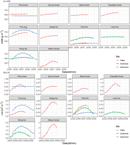
Among the VTs, pine forest, mixed forest, and lawn fens had nearly stable AGBs throughout the growing season, while the other VTs composed mostly of deciduous species showed a strong seasonal amplitude (). Seasonal amplitudes of AGB and LAI varied within the VTs from different sites. For instance, LAIs of string fens had greater seasonal amplitude in Kaamanen than in Sodankylä, i.e. 1 and 0.5 m2 m−2, respectively.
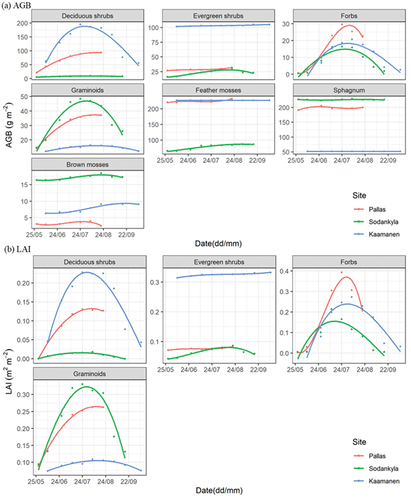
Figure 4. The seasonal development of (a) aboveground biomass (AGB) and (b) leaf area index (LAI) by vegetation types (VTs) at the study sites.
The three deciduous vascular plant PFTs (deciduous shrubs, forbs, graminoids) had clear seasonal trajectories in both AGB and LAI, while little changes were observed in the seasonal patterns of AGB and LAI of evergreen shrubs and mosses (). The seasonality of individual PFTs still differed between sites. For example, the AGB and LAI of forbs peaked at an earlier date at the southernmost site, i.e. Sodankylä, where DD5 accumulated more rapidly and to a higher level than at the other sites ( and Fig. S1).
Figure 5. The seasonal development of (a) aboveground biomass (AGB) and (b) leaf area index (LAI) by plant functional types (PFTs) at the study sites.
4.2. Predictive performance of random forest regressions
The RF regressions yielded a mean R2 of 48.5–56.1% for LAI and 24.2–50.2% for AGB (). The Sodankylä models had a higher R2 and lower error rates than the Pallas models ( and ). The AGB model for Pallas performed well only for certain VTs, while the LAI model had a better fit (). The two-site models had a performance in between the single-site models, with their performance closer to that of the Pallas models. However, they failed to reach acceptable prediction rates in Sodankylä, so we finally adopted single-site regression models to generate the following spatiotemporal AGB and LAI maps. In general, RF predicted relatively inaccurately low (<500 g m−2) and high AGB (>750 g m−2) and high LAI (>2 m2 m−2) ().
Figure 6. Scatterplots of field- and S2- estimated aboveground biomass (AGB) and leaf area index (LAI), which are color-coded by vegetation types (VTs). The S2 estimations derived from two types of RF regression models: the single-site model (single-site M) and two-site model (two-site M), respectively. In the figure, the solid lines represent the 1:1 line; and the dashed lines indicate linear regression fits between predicted and observed values.
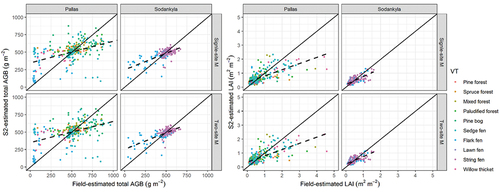
Table 3. Random Forest regression results for ground vegetation total aboveground biomass (AGB) and leaf area index (LAI).
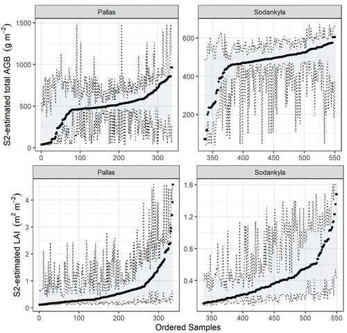
The prediction uncertainty for single-site RF models, measured by 0.025 (the lower boundary) and 0.0975 (the upper boundary) quantiles with QRF in , indicates that Sodankylä had relatively narrower prediction interval widths (the dashed grey shadows in ) for both AGB and LAI compared to Pallas. Furthermore, the estimated AGB and LAI in the middle value range appeared to have a relatively narrower range of prediction possibilities compared particularly to low AGB (<500 g m2 at both sites) and high LAI (>0.8 m2 m2 in Pallas or >0.4 m2 in Sodankylä).
Figure 7. The 95% prediction intervals of S2-estimated aboveground biomass (AGB) and leaf area index (LAI) based on single-site RF regression models, which are shown in . The grey shaded regions represent the lower and upper boundaries of the 0.025 and 0.975 quantiles, respectively. For better visualization, the estimated samples are sorted by their AGB or LAI values.
4.3. Modelled spatiotemporal patterns of AGB and LAI
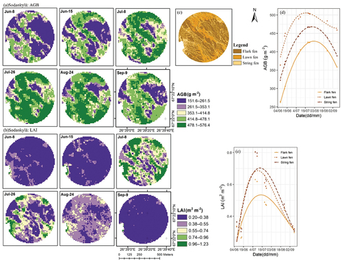
Sentinel-2-based modelled AGB and LAI peaked approximately 21 d and 10 d later than the field-measured ones, respectively (). The seasonal development of AGB and LAI in Pallas was mostly stable in forest VTs, though spruce forests in the south-eastern corner of Pallas showed slight variations in AGB, with accumulation beginning in mid-June and senescence in August (). On the contrary, AGB and LAI within peatland-dominated areas were low in June, gradually increased until late July, and were senescent in August (). In Sodankylä, AGB and LAI had rather visible spatial patterns, with lowest values recorded in flarks (). The three VTs had similar temporal AGB trends, while LAI was spatially uniform before July, but strings and lawns subsequently had higher LAIs than flarks did ().
Figure 8. Comparison between field-measured and S2-modelled (based on single-site models) seasonal patterns of (a) aboveground biomass (AGB) and (b) leaf area index (LAI).

Figure 9. Sentinel-2-based spatiotemporal maps (with 10-m spatial resolution) of (a) aboveground biomass (AGB), and (b) leaf area index (LAI); (c) land cover classification map, which is the same as in ; and Sentinel-2-based average seasonal line trends of (d) AGB and (e) LAI by VTs (vegetation types), at Pallas.
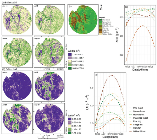
Figure 10. Sentinel-2-based spatiotemporal maps (with 10-m spatial resolution) of (a) aboveground biomass (AGB) and (b) leaf area index (LAI); (c) land cover classification map, which is the same as in ; and Sentinel-2-based average seasonal line trends of (d) AGB and (e) LAI by VTs (vegetation types), at Sodankylä.
5. Discussion
5.1. Field-measured AGB and LAI patterns
We found the ground vegetation total AGB and LAI to follow a unimodal seasonality and their peaking dates to differ (), which is in line with previous studies (Heiskanen et al. Citation2012; Juutinen et al. Citation2017; Wang et al. Citation2019; Wilson et al. Citation2007). For example, the LAI peaking date of Lompojänkkä in this study corroborates the results of Raivonen et al. (Citation2015), and various AGB peaks within boreal forests are consistent with the results of Ding et al. (Citation2021). AGB and LAI had distinct seasonal patterns among VTs (), echoing other studies (Arndal et al. Citation2009; Heiskanen et al. Citation2012; Korrensalo et al. Citation2020; Raivonen et al. Citation2015). Specifically, we identified that fen VTs have greater seasonal variations than forest VTs, which is attributed to the phenology of dominated PFT, i.e. a larger proportion of deciduous vegetation in fens vs. evergreen shrub forests (Fig. S4) (Arndal et al. Citation2009; Rautiainen and Heiskanen Citation2013). Moreover, peatland VTs still vary considerably from each other, as also previously reported by (Korrensalo et al. Citation2020), who showed string fens (or hummocks) to have higher AGB and LAI peaking values and stronger seasonal variation than lawns (Figs. S6 and S7).
PFT-specified AGB and LAI exhibited apparent seasonal trajectories. Apart from evergreen shrubs, vascular PFTs had unimodal curves, while moss AGB remained almost steady throughout the season (). However, our moss height field measurements were not planned to measure differences of some millimetres, which are evidently occurring during the growing season. On the one hand, vascular PFTs showed differences; for example, graminoid LAI had a later peaking date than that of forbs and deciduous shrubs. On the other hand, seasonal trends of PFT-specific AGB and LAI were still disparate by sites and VTs (). For instance, shrubs abundantly prevail in Kaamanen, while forbs and mosses form the major VTs in Sodankylä (Figs. S3 and S4). Also, vascular PFTs store more AGB in strings than in lawns, while Sphagnum in flarks accumulate more mass than species in drier areas (Fig. S6), corresponding with earlier studies (Gunnarsson Citation2005; Kosykh et al. Citation2008; Laine et al. Citation2012; Mäkiranta et al. Citation2018; Murphy, Mckinley, and Moore Citation2009). In this study, we did not include the moss component in the LAI estimations, as there is neither a generally accepted method for measuring this in the field nor can their LAI be directly compared with that of vascular plants. Mosses with foliage consisting of miniature leaves actually have a very large input on LAI (Niinemets and Tobias Citation2019); thus, their role obviously needs more attention in future remote sensing-based vegetation and carbon exchange studies (Shi et al. Citation2021).
5.2. Spatiotemporal patterns of AGB and LAI based on Sentinel-2
In S2-analysis, single-site models performed generally better than two-site ones (). Due to the high spatial heterogeneity and contrasting vegetation composition within boreal ecosystems, it is reasonable that two-site models did not yield acceptable prediction rates (Alexandridis, Ovakoglou, and Clevers Citation2020; Junttila et al. Citation2021; Räsänen et al. Citation2021). Sodankylä models had better prediction performance than Pallas models, probably related to Sodankylä being nearly entirely a treeless peatland, while Pallas includes both treeless peatland areas and forests with relatively dense tree crown cover (typically 20–50%). The tree canopy layer greatly hampers the remote detectability of ground layer vegetation (Eriksson et al. Citation2006; Rautiainen and Heiskanen Citation2013). Moreover, covering broader landscapes from boreal forests to peatlands implies higher spatial variations, while a limited number and manual selection of field plots do not perfectly represent ground vegetation conditions ( and ). In other words, the study area in Pallas was five times larger than that of Sodankylä, and the number of plots in forest VTs in Pallas was relatively low.
Despite S2-modelled AGB and LAI following a similar unimodal trend with field-based patterns, the modelled ones had earlier seasonal peaks (). Due to the difference between field-measured and S2 variables, i.e. the %-cover and number of PFTs representing photosynthetic productivity vs. remotely sensed reflectance, field-measured vegetation seasonal dynamics differ from S2 modelled ones (Tian et al. Citation2021; Vrieling et al. Citation2018). AGB and LAI measured in the field rely on human visual observations and are limited to a few plant individuals, while the dozens of remote sensing metrics applied reflect a mixed response to vegetation changes, leading to internal discrepancies between these two data types. Moreover, field-measured AGB and LAI directly express the ground layer vegetation () within 0.2-m2 plots but 100-m2 S2 pixels are a mixture of vegetation information (e.g. leaf area, leaf colour, and the VT mixture), other land covers, and background noises (e.g. periodical flooding). The spatial resolution mismatch therefore brings uncertainty to regression modelling. Furthermore, the seasonal trajectory differences between boreal forests and peatlands and the combined effect of ground flooding conditions indicate considerable difficulties in catching vegetation phenological phases using remote sensing (Thapa, Millan, and Eklundh Citation2021). Overall, the phenological date variations of AGB (21 d) and LAI (10 d) between field- and S2-based estimations () correspond with previous reports (Descals et al. Citation2020; Thapa, Millan, and Eklundh Citation2021; Tian et al. Citation2021; Vrieling et al. Citation2018), which have reported a temporal difference of 8–30 d.
We adopted site-specific models for predicting and generating AGB and LAI maps, and their accuracy was close to previous results, where R2 has been 47–89% (Amin et al. Citation2018; Fassnacht et al. Citation2021; Pang et al. Citation2022; Puliti et al. Citation2020; Räsänen et al. Citation2021; Wang et al. Citation2019). Regression models performed poorly with low and high AGB and LAI values (). Similar issues have also been pointed out by other studies. Some studies have indicated that RF may not predict extreme values accurately (Fassnacht et al. Citation2021; Wang et al. Citation2022), while others have reported that S2-based estimations were relatively inaccurate during vegetation green-up and senescence periods (Tian et al. Citation2021; Vrieling et al. Citation2018). On the one hand, following the vegetation phenological cycle, low AGB values occurred in the early or late growing season (in early June or mid-August), when vascular plant leaves have just begun turning green or senescencing, storing low amounts of AGB (), but the presence of a non-photosynthetic top layer (flowers, stems, seed heads) may interfere with ground radiance, delivering systematic errors to regression models. On the other hand, high ground vegetation AGB values were found in forest areas. Due to rather small seasonal amplitudes of evergreen boreal forest phenology along with the dense canopy layer (Misra, Cawkwell, and Wingler Citation2020), S2 data seem to overestimate ground vegetation AGB in these areas. Generally, S2 models performed fairly well for extracting seasonal trends and phenological dates in Sodankylä, suggesting the great potential of applying S2 data to open peatlands. Furthermore, echoing early studies (Majasalmi and Rautiainen Citation2016; Räsänen et al. Citation2020; Wang et al. Citation2019), we also clarified that LAI was detected with higher accuracy than AGB; clear seasonal patterns in LAI maps were observed especially in peatland-dominated areas ().
6. Conclusions
We have explored ground vegetation phenology with field observations and S2 satellite images across boreal ecosystems. Our results show that the seasonality of AGB and LAI vary greatly between VTs, particularly in fens, depending on whether the dominant PFTs are deciduous or evergreen. Besides evergreen shrubs and mosses, the seasonality of other PFTs follow a unimodal curve. Our results also indicate that LAI peaks ca. two weeks earlier than AGB. Our results further reveal that the field measurements can be upscaled with S2 regression models with acceptable accuracy. With the help of satellite-data-based upscaling, we illustrate that there is a good ability to capture spatiotemporal patterns of AGB and LAI and that the AGB and LAI phenology differs between VTs at the landscape scale. Therefore, we suggest that S2 time series data, with a 10-m spatial resolution, allows monitoring ground vegetation seasonality in treeless boreal ecosystems.
With the advancements in artificial intelligence, machine and deep learning, and remote sensing sensors, future research can further explore how to improve the prediction accuracy in seasonal AGB and LAI estimates. Particularly, the inclusion of other remote sensing or ancillary data could enhance model performance. Possible data sources include Sentinel-1 or other SAR data sensitive to soil moisture conditions and surface structure, lidar capable for capturing 3D topographical and vegetation information, and higher spatial resolution optical data. However, when producing spatial estimates of the AGB and LAI development over a growing season, majority of the data should have multiple observations from a single growing season.
Pang_Yuwen_Appendix_Revised_finnal.docx
Download MS Word (2.5 MB)Acknowledgements
We thank all who participated in the field data collection: Jani Antila, Holtti Hakonen, Viivi Lindholm, and Pauliina Wäli. YP acknowledges the support of the China Scholarship Council for her PhD research [grant number 202008330336] at the University of Helsinki. MV acknowledges funding from the Academy of Finland [grant number 338631]. Field data collection was funded by the Academy of Finland [grant numbers 296423, 308513]. Open access was funded by the Helsinki University Library.
Disclosure statement
No potential conflict of interest was reported by the author(s).
Data Availability statement
The Sentinel-2 data used in this study is available at https://developers.google.com/earth-engine/datasets/catalog/COPERNICUS_S2_SR. An example JavaScript code of generating AGB and LAI spatiotemporal maps is available at https://code.earthengine.google.com/d402cc0f59cb90f8d53a802871f5010d. The field vegetation inventory data and the produced AGB and LAI maps are available from the corresponding author upon reasonable request.
Supplementary material
Supplemental data for this article can be accessed online at https://doi.org/10.1080/01431161.2023.2234093.
Additional information
Funding
References
- Alexandridis, T. K., G. Ovakoglou, and J. G. P. W. Clevers. 2020. “Relationship Between MODIS EVI and LAI Across Time and Space.” Geocarto International 35 (13): 1385–1399. https://doi.org/10.1080/10106049.2019.1573928.
- Amin, E., J. Verrelst, J. P. Rivera-Caicedo, N. Pasqualotto, J. Delegido, A. R. Verdu, and J. Moreno 2018. “The Sensagri Sentinel-2 Lai Green and Brown Product: From Algorithm Development Towards Operational Mapping.” IGARSS 2018 - 2018 IEEE International Geoscience and Remote Sensing Symposium, 1822–1825. Valencia, Spain. https://doi.org/10.1109/IGARSS.2018.8518938
- Arndal, M. F., L. Illeris, A. Michelsen, K. Albert, M. Tamstorf, and B. U. Hansen. 2009. “Seasonal Variation in Gross Ecosystem Production, Plant Biomass, and Carbon and Nitrogen Pools in Five High Arctic Vegetation Types.” Arctic, Antarctic, and Alpine Research 41 (2): 164–173. https://doi.org/10.1657/1938-4246-41.2.164.
- Arroyo-Mora, J. P., M. Kalacska, R. Soffer, G. Ifimov, G. Leblanc, E. S. Schaaf, and O. Lucanus. 2018. “Evaluation of Phenospectral Dynamics with Sentinel-2A Using a Bottom-Up Approach in a Northern Ombrotrophic Peatland.” Remote Sensing of Environment 216:544–560. https://doi.org/10.1016/j.rse.2018.07.021.
- Astola, H., T. Hame, L. Sirro, M. Molinier, and J. Kilpi. 2019. “Comparison of Sentinel-2 and Landsat 8 Imagery for Forest Variable Prediction in Boreal Region.” Remote Sensing of Environment 223:257–273. https://doi.org/10.1016/j.rse.2019.01.019.
- Aurela, M., A. Lohila, J. P. Tuovinen, J. Hatakka, T. Penttila, and T. Laurila. 2015. “Carbon Dioxide and Energy Flux Measurements in Four Northern-Boreal Ecosystems at Pallas.” Boreal Environment Research 20 (4): 455–473.
- Bhatti, S., S. R. Ahmad, M. Asif, I. U. Farooqi, and F. Fassnacht. 2022. “Estimation of Aboveground Carbon Stock Using Sentinel-2A Data and Random Forest Algorithm in Scrub Forests of the Salt Range, Pakistan.” Forestry: An International Journal of Forest Research 96 (1): 104–120. https://doi.org/10.1093/forestry/cpac036.
- Bradshaw, C. J. A., and I. G. Warkentin. 2015. “Global Estimates of Boreal Forest Carbon Stocks and Flux.” Global and Planetary Change 128:24–30. https://doi.org/10.1016/j.gloplacha.2015.02.004.
- Breiman, L. 2001. “Random Forests.” Machine Learning 45 (1): 5–32. https://doi.org/10.1023/A:1010933404324.
- Breiman, L. 2003. Manual for Setting Up, Using, and Understanding Random Forest V4. 0. https://www.stat.berkeley.edu/~breiman/Using_random_forests_v4.0.pdf.
- Canovas-Garcia, F., F. Alonso-Sarria, F. Gomariz-Castillo, and F. Onate-Valdivieso. 2017. “Modification of the Random Forest Algorithm to Avoid Statistical Dependence Problems When Classifying Remote Sensing Imagery.” Computers & Geosciences 103:1–11. https://doi.org/10.1016/j.cageo.2017.02.012.
- Chen, J. M., and T. A. Black. 1992. “Defining Leaf-Area Index for Non-Flat Leaves.” Plant Cell and Environment 15 (4): 421–429. https://doi.org/10.1111/j.1365-3040.1992.tb00992.x.
- Czapiewski, S., and D. Szuminska. 2022. “An Overview of Remote Sensing Data Applications in Peatland Research Based on Works from the Period 2010–2021.” Land 11 (1). https://doi.org/10.3390/land11010024.
- Descals, A., A. Verger, G. F. Yin, and J. Penuelas. 2020. “Improved Estimates of Arctic Land Surface Phenology Using Sentinel-2 Time Series.” Remote Sensing 12 (22). https://doi.org/10.3390/rs12223738.
- Ding, Y. Y., J. Leppalammi-Kujansuu, M. Salemaa, P. Schiestl-Aalto, L. Kulmala, L. Ukonmaanaho, P. Nojd, et al. 2021. “Distinct Patterns of Below- and Aboveground Growth Phenology and Litter Carbon Inputs Along a Boreal Site Type Gradient.” Forest Ecology and Management 489:119081. https://doi.org/10.1016/j.foreco.2021.119081.
- Eriksson, H. M., L. Eklundh, A. Kuusk, and T. Nilson. 2006. “Impact of Understory Vegetation on Forest Canopy Reflectance and Remotely Sensed LAI Estimates.” Remote Sensing of Environment 103 (4): 408–418. https://doi.org/10.1016/j.rse.2006.04.005.
- Fan, X. Y., G. J. He, W. Y. Zhang, T. F. Long, X. M. Zhang, G. Z. Wang, G. Sun, et al. 2022. “Sentinel-2 Images Based Modeling of Grassland Above-Ground Biomass Using Random Forest Algorithm: A Case Study on the Tibetan Plateau.” Remote Sensing 14 (21): 5321. https://doi.org/10.3390/rs14215321.
- Fassnacht, F. E., J. Poblete-Olivares, L. Rivero, J. Lopatin, A. Ceballos-Comisso, and M. Galleguillos. 2021. “Using Sentinel-2 and Canopy Height Models to Derive a Landscape-Level Biomass Map Covering Multiple Vegetation Types.” International Journal of Applied Earth Observation and Geoinformation 94:102236. https://doi.org/10.1016/j.jag.2020.102236.
- Gorelick, N., M. Hancher, M. Dixon, S. Ilyushchenko, D. Thau, and R. Moore. 2017. “Google Earth Engine: Planetary-Scale Geospatial Analysis for Everyone.” Remote Sensing of Environment 202:18–27. https://doi.org/10.1016/j.rse.2017.06.031.
- Gunnarsson, U. 2005. “Global Patterns of Sphagnum Productivity.” Journal of Bryology 27 (3): 269–279. https://doi.org/10.1179/174328205X70029.
- Haapala, J. K., S. K. Morsky, S. Saarnio, R. Rinnan, H. Suokanerva, E. Kyro, K. Latola, P. J. Martikanen, T. Holopainen, and J. Silvola. 2009. “Carbon Dioxide Balance of a Fen Ecosystem in Northern Finland Under Elevated UV-B Radiation.” Global Change Biology 15 (4): 943–954. https://doi.org/10.1111/j.1365-2486.2008.01785.x.
- Heiskanen, J., M. Rautiainen, P. Stenberg, M. Mottus, V. H. Vesanto, L. Korhonen, and T. Majasalmi. 2012. “Seasonal Variation in MODIS LAI for a Boreal Forest Area in Finland.” Remote Sensing of Environment 126:104–115. https://doi.org/10.1016/j.rse.2012.08.001.
- Helbig, M., J. M. Waddington, P. Alekseychik, B. D. Amiro, M. Aurela, A. G. Barr, T. A. Black, et al. 2020. “Increasing Contribution of Peatlands to Boreal Evapotranspiration in a Warming Climate.” Nature Climate Change 10 (6): 555–560. https://doi.org/10.1038/s41558-020-0763-7.
- Hengl, T., M. Nussbaum, M. N. Wright, G. B. M. Heuvelink, and B. Graler. 2018. “Random Forest as a Generic Framework for Predictive Modeling of Spatial and Spatio-Temporal Variables.” PeerJ 6:6. https://doi.org/10.7717/peerj.5518.
- Junttila, S., J. Kelly, N. Kljun, M. Aurela, L. Klemedtsson, A. Lohila, M. B. Nilsson, et al. 2021. “Upscaling Northern Peatland CO2 Fluxes Using Satellite Remote Sensing Data.” Remote Sensing 13 (4): 818. https://doi.org/10.3390/rs13040818.
- Juutinen, S., T. Virtanen, V. Kondratyev, T. Laurila, M. Linkosalmi, J. Mikola, J. Nyman, A. Rasanen, J. P. Tuovinen, and M. Aurela. 2017. “Spatial Variation and Seasonal Dynamics of Leaf-Area Index in the Arctic Tundra-Implications for Linking Ground Observations and Satellite Images.” Environmental Research Letters 12 (9): 095002. https://doi.org/10.1088/1748-9326/aa7f85.
- Koebsch, F., O. Sonnentag, J. Jarveoja, M. Peltoniemi, P. Alekseychik, M. Aurela, A. N. Arslan, et al. 2020. “Refining the Role of Phenology in Regulating Gross Ecosystem Productivity Across European Peatlands.” Global Change Biology 26 (2): 876–887. https://doi.org/10.1111/gcb.14905.
- Korhonen, L., P. Packalen, and M. Rautiainen. 2017. “Comparison of Sentinel-2 and Landsat 8 in the Estimation of Boreal Forest Canopy Cover and Leaf Area Index.” Remote Sensing of Environment 195:259–274. https://doi.org/10.1016/j.rse.2017.03.021.
- Korrensalo, A., L. Kettunen, R. Laiho, P. Alekseychik, T. Vesala, I. Mammarella, E.-S. Tuittila, S. Roxburgh, and S. Roxburgh. 2018. “Boreal Bog Plant Communities Along a Water Table Gradient Differ in Their Standing Biomass but Not Their Biomass Production.” Journal of Vegetation Science 29 (2): 136–146. https://doi.org/10.1111/jvs.12602.
- Korrensalo, A., L. Mehtatalo, P. Alekseychik, S. Uljas, I. Mammarella, T. Vesala, and E. S. Tuittila. 2020. “Varying Vegetation Composition, Respiration and Photosynthesis Decrease Temporal Variability of the CO2 Sink in a Boreal Bog.” Ecosystems 23 (4): 842–858. https://doi.org/10.1007/s10021-019-00434-1.
- Kosykh, N. P., N. G. Koronatova, N. B. Naumova, and A. A. Titlyanova. 2008. “Above-And Below-Ground Phytomass and Net Primary Production in Boreal Mire Ecosystems of Western Siberia.” Wetlands Ecology and Management 16 (2): 139–153. https://doi.org/10.1007/s11273-007-9061-7.
- Laine, A. M., J. Bubier, T. Riutta, M. B. Nilsson, T. R. Moore, H. Vasander, and E. S. Tuittila. 2012. “Abundance and Composition of Plant Biomass as Potential Controls for Mire Net Ecosytem CO2 Exchange.” Botany 90 (1): 63–74. https://doi.org/10.1139/b11-068.
- Laitinen, J., J. Oksanen, E. Kaakinen, M. Parviainen, M. Kuttim, and R. Ruuhijarvi. 2017. “Regional and Vegetation-Ecological Patterns in Northern Boreal Flark Fens of Finnish Lapland: Analysis from a Classic Material.” Annales Botanici Fennici 54 (1–3): 179–195. https://doi.org/10.5735/085.054.0327.
- Liaw, A., and M. Wiener. 2002. “Classification and Regression by randomForest.” R News 2 (3): 18–22.
- Linkosalmi, M., J. P. Tuovinen, O. Nevalainen, M. Peltoniemi, C. M. Tanis, A. N. Arslan, J. Rainne, A. Lohila, T. Laurila, and M. Aurela. 2022. “Tracking Vegetation Phenology of Pristine Northern Boreal Peatlands by Combining Digital Photography with CO2 Flux and Remote Sensing Data.” Biogeosciences 19 (19): 4747–4765. https://doi.org/10.5194/bg-19-4747-2022.
- Lohila, A., T. Penttila, S. Jortikka, T. Aalto, P. Anttila, E. Asmi, M. Aurela, et al. 2015. “Preface to the Special Issue on Integrated Research of Atmosphere, Ecosystems and Environment at Pallas.” Boreal Environment Research 20 (4): 431–454.
- Lyons, C. L., B. A. Branfireun, J. Mclaughlin, and Z. Lindo. 2020. “Simulated Climate Warming Increases Plant Community Heterogeneity in Two Types of Boreal Peatlands in North–Central Canada.” Journal of Vegetation Science 31 (5): 908–919. https://doi.org/10.1111/jvs.12912.
- Maanavilja, L., T. Riutta, M. Aurela, M. Pulkkinen, T. Laurila, and E. S. Tuittila. 2011. “Spatial Variation in CO2 Exchange at a Northern Aapa Mire.” Biogeochemistry 104 (1–3): 325–345. https://doi.org/10.1007/s10533-010-9505-7.
- Macdonald, R. L., J. M. Burke, H. Y. H. Chen, and E. E. Prepas. 2012. “Relationship Between Aboveground Biomass and Percent Cover of Ground Vegetation in Canadian Boreal Plain Riparian Forests.” Forest Science 58 (1): 47–53. https://doi.org/10.5849/forsci.10-129.
- Majasalmi, T., and M. Rautiainen. 2016. “The Potential of Sentinel-2 Data for Estimating Biophysical Variables in a Boreal Forest: A Simulation Study.” Remote Sensing Letters 7 (5): 427–436. https://doi.org/10.1080/2150704X.2016.1149251.
- Mäkiranta, P., R. Laiho, L. Mehtatalo, P. Strakova, J. Sormunen, K. Minkkinen, T. Penttila, H. Fritze, and E. S. Tuittila. 2018. “Responses of Phenology and Biomass Production of Boreal Fens to Climate Warming Under Different Water-Table Level Regimes.” Global Change Biology 24 (3): 944–956. https://doi.org/10.1111/gcb.13934.
- Malamiri, H. R. G., H. Zare, I. Rousta, H. Olafsson, E. I. Verdiguier, H. Zhang, and T. D. Mushore. 2020. “Comparison of Harmonic Analysis of Time Series (HANTS) and Multi-Singular Spectrum Analysis (M-SSA) in Reconstruction of Long-Gap Missing Data in NDVI Time Series.” Remote Sensing 12 (17): 2747. https://doi.org/10.3390/rs12172747.
- Maleki, M., N. Arriga, J. M. Barrios, S. Wieneke, Q. Liu, J. Penuelas, I. A. Janssens, and M. Balzarolo. 2020. “Estimation of Gross Primary Productivity (GPP) Phenology of a Short-Rotation Plantation Using Remotely Sensed Indices Derived from Sentinel-2 Images.” Remote Sensing 12 (13): 12. https://doi.org/10.3390/rs12132104.
- Mcpartland, M. Y., R. A. Montgomery, P. J. Hanson, J. R. Phillips, R. Kolka, and B. Palik. 2020. “Vascular Plant Species Response to Warming and Elevated Carbon Dioxide in a Boreal Peatland.” Environmental Research Letters 15 (12): 124066. https://doi.org/10.1088/1748-9326/abc4fb.
- Meinshausen, N. 2006. “Quantile Regression Forests.” Journal of Machine Learning Research 7 (35): 983–999.
- Mentch, L., and G. Hooker. 2016. “Quantifying Uncertainty in Random Forests via Confidence Intervals and Hypothesis Tests.” Journal of Machine Learning Research 17 (1): 841–881.
- Misra, G., F. Cawkwell, and A. Wingler. 2020. “Status of Phenological Research Using Sentinel-2 Data: A Review.” Remote Sensing 12 (17): 2760. https://doi.org/10.3390/rs12172760.
- Mörsky, S. K., J. K. Haapala, R. Rinnan, S. Saarnio, H. Suokanerva, K. Latola, E. Kyro, J. Silvola, T. Holopainen, and P. J. Martikainen. 2012. “Minor Long-Term Effects of Ultraviolet-B Radiation on Methane Dynamics of a Subarctic Fen in Northern Finland.” Biogeochemistry 108 (1–3): 233–243. https://doi.org/10.1007/s10533-011-9593-z.
- Murphy, M. T., A. Mckinley, and T. R. Moore. 2009. “Variations in Above- and Below-Ground Vascular Plant Biomass and Water Table on a Temperate Ombrotrophic Peatland.” Botany 87 (9): 845–853. https://doi.org/10.1139/B09-052.
- Niinemets, U., and M. Tobias. 2019. “Canopy Leaf Area Index at Its Higher End: Dissection of Structural Controls from Leaf to Canopy Scales in Bryophytes.” New Phytologist 223 (1): 118–133. https://doi.org/10.1111/nph.15767.
- Pang, Y. W., A. Rasanen, V. Lindholm, M. Aurela, and T. Virtanen. 2022. “Detecting Peatland Vegetation Patterns with Multi-Temporal Field Spectroscopy.” Giscience & Remote Sensing 59 (1): 2111–2126. https://doi.org/10.1080/15481603.2022.2152303.
- Pearson, M., T. Penttila, L. Harjunpaa, R. Laiho, J. Laine, T. Sarjala, K. Silvan, and N. Silvan. 2015. “Effects of Temperature Rise and Water-Table-Level Drawdown on Greenhouse Gas Fluxes of Boreal Sedge Fens.” Boreal Environment Research 20 (4): 489–505.
- Peichl, M., M. Gazovic, I. Vermeij, E. De Goede, O. Sonnentag, J. Limpens, and M. B. Nilsson. 2018. “Peatland Vegetation Composition and Phenology Drive the Seasonal Trajectory of Maximum Gross Primary Production.” Scientific Reports 8 (1). https://doi.org/10.1038/s41598-018-26147-4.
- Peterka, T., M. Hajek, M. Jirousek, B. Jimenez-Alfaro, L. Aunina, A. Bergamini, D. Dite, et al. 2017. “Formalized Classification of European Fen Vegetation at the Alliance Level.” Applied Vegetation Science 20 (1): 124–142. https://doi.org/10.1111/avsc.12271.
- Poggio, L., L. M. De Sousa, N. H. Batjes, G. B. M. Heuvelink, B. Kempen, E. Ribeiro, and D. Rossiter. 2021. “SoilGrids 2.0: Producing Soil Information for the Globe with Quantified Spatial Uncertainty.” Soil 7:217–240. https://doi.org/10.5194/soil-7-217-2021.
- Pohjanmies, T., N. Genikova, J. P. Hotanen, H. Ilvesniemi, A. Kryshen, S. Moshnikov, J. Oksanen, et al. 2021. “Site Types Revisited: Comparison of Traditional Russian and Finnish Classification Systems for European Boreal Forests.” Applied Vegetation Science 24 (1). https://doi.org/10.1111/avsc.12525.
- Powell, S. L., W. B. Cohen, S. P. Healey, R. E. Kennedy, G. G. Moisen, K. B. Pierce, and J. L. Ohmann. 2010. “Quantification of Live Aboveground Forest Biomass Dynamics with Landsat Time-Series and Field Inventory Data: A Comparison of Empirical Modeling Approaches.” Remote Sensing of Environment 114 (5): 1053–1068. https://doi.org/10.1016/j.rse.2009.12.018.
- Puliti, S., M. Hauglin, J. Breidenbach, P. Montesano, C. S. R. Neigh, J. Rahlf, S. Solberg, T. F. Klingenberg, and R. Astrup. 2020. “Modelling Above-Ground Biomass Stock Over Norway Using National Forest Inventory Data with ArcticDem and Sentinel-2 Data.” Remote Sensing of Environment 236:111501. https://doi.org/10.1016/j.rse.2019.111501.
- Raivonen, M., P. Makiranta, A. Lohila, S. Juutinen, T. Vesala, and E. S. Tuittila. 2015. “A Simple CO2 Exchange Model Simulates the Seasonal Leaf Area Development of Peatland Sedges.” Ecological Modelling 314:32–43. https://doi.org/10.1016/j.ecolmodel.2015.07.008.
- Räsänen, A., M. Aurela, S. Juutinen, T. Kumpula, A. Lohila, T. Penttila, T. Virtanen, N. Horning, and J. Zhang. 2020. “Detecting Northern Peatland Vegetation Patterns at Ultra-High Spatial Resolution.” Remote Sensing in Ecology and Conservation 6 (4): 457–471. https://doi.org/10.1002/rse2.140.
- Räsänen, A., S. Juutinen, M. Kalacska, M. Aurela, P. Heikkinen, K. Maenpaa, A. Rimali, and T. Virtanen. 2020. “Peatland Leaf-Area Index and Biomass Estimation with Ultra-High Resolution Remote Sensing.” Giscience & Remote Sensing 57 (7): 943–964. https://doi.org/10.1080/15481603.2020.1829377.
- Räsänen, A., T. Manninen, M. Korkiakoski, A. Lohila, and T. Virtanen. 2021. “Predicting Catchment-Scale Methane Fluxes with Multi-Source Remote Sensing.” Landscape Ecology 36 (4): 1177–1195. https://doi.org/10.1007/s10980-021-01194-x.
- Räsänen, A., and T. Virtanen. 2019. “Data and Resolution Requirements in Mapping Vegetation in Spatially Heterogeneous Landscapes.” Remote Sensing of Environment 230:111207. https://doi.org/10.1016/j.rse.2019.05.026.
- Räsänen, A., J. Wagner, G. Hugelius, and T. Virtanen. 2021. “Aboveground Biomass Patterns Across Treeless Northern Landscapes.” International Journal of Remote Sensing 42 (12): 4536–4561. https://doi.org/10.1080/01431161.2021.1897187.
- Rautiainen, M., and J. Heiskanen. 2013. “Seasonal Contribution of Understory Vegetation to the Reflectance of a Boreal Landscape at Different Spatial Scales.” Ieee Geoscience and Remote Sensing Letters 10 (4): 923–927. https://doi.org/10.1109/LGRS.2013.2247560.
- Richardson, A. D., T. F. Keenan, M. Migliavacca, Y. Ryu, O. Sonnentag, and M. Toomey. 2013. “Climate Change, Phenology, and Phenological Control of Vegetation Feedbacks to the Climate System.” Agricultural and Forest Meteorology 169:156–173. https://doi.org/10.1016/j.agrformet.2012.09.012.
- Schiefer, F., S. Schmidtlein, A. Frick, J. Frey, R. Klinke, K. Zielewska-Büttner, S. Junttila, A. Uhl, and T. Kattenborn. 2023. “UAV-Based Reference Data for the Prediction of Fractional Cover of Standing Deadwood from Sentinel Time Series.” ISPRS Open Journal of Photogrammetry and Remote Sensing 8:100034. https://doi.org/10.1016/j.ophoto.2023.100034.
- Shi, X. Y., D. M. Ricciuto, P. E. Thornton, X. F. Xu, F. M. Yuan, R. J. Norby, A. P. Walker, et al. 2021. “Extending a Land-Surface Model with Sphagnum Moss to Simulate Responses of a Northern Temperate Bog to Whole Ecosystem Warming and Elevated CO2.” Biogeosciences 18:467–486. https://doi.org/10.5194/bg-18-467-2021.
- Skidmore, A. K., N. C. Coops, E. Neinavaz, A. Ali, M. E. Schaepman, M. Paganini, W. D. Kissling, et al. 2021. “Priority List of Biodiversity Metrics to Observe from Space.” Nature Ecology & Evolution 5:896–906. https://doi.org/10.1038/s41559-021-01451-x.
- Thapa, S., V. E. G. Millan, and L. Eklundh. 2021. “Assessing Forest Phenology: A Multi-Scale Comparison of Near-Surface (UAV, Spectral Reflectance Sensor, PhenoCam) and Satellite (MODIS, Sentinel-2) Remote Sensing.” Remote Sensing 13 (8): 1597. https://doi.org/10.3390/rs13081597.
- Tian, J., B. A. Branfireun, and Z. Lindo. 2020. “Global Change Alters Peatland Carbon Cycling Through Plant Biomass Allocation.” Plant and Soil 455 (1–2): 53–64. https://doi.org/10.1007/s11104-020-04664-4.
- Tian, F., Z. Z. Cai, H. X. Jin, K. Hufkens, H. Scheifinger, T. Tagesson, B. Smets, et al. 2021. “Calibrating Vegetation Phenology from Sentinel-2 Using Eddy Covariance, PhenoCam, and PEP725 Networks Across Europe.” Remote Sensing of Environment 260. https://doi.org/10.1016/j.rse.2021.112456.
- Vaysse, K., and P. Lagacherie. 2017. “Using Quantile Regression Forest to Estimate Uncertainty of Digital Soil Mapping Products.” Geoderma 291:55–64. https://doi.org/10.1016/j.geoderma.2016.12.017.
- Verwijst, T., and B. Telenius. 1999. “Biomass Estimation Procedures in Short Rotation Forestry.” Forest Ecology and Management 121 (1–2): 137–146. https://doi.org/10.1016/S0378-11279800562-3.
- Vrieling, A., M. Meroni, R. Darvishzadeh, A. K. Skidmore, T. J. Wang, R. Zurita-Milla, K. Oosterbeek, B. O’Connor, and M. Paganini. 2018. “Vegetation Phenology from Sentinel-2 and Field Cameras for a Dutch Barrier Island.” Remote Sensing of Environment 215:517–529. https://doi.org/10.1016/j.rse.2018.03.014.
- Wang, Q., N. A. Putri, Y. Gan, and G. M. Song. 2022. “Combining Both Spectral and Textural Indices for Alleviating Saturation Problem in Forest LAI Estimation Using Sentinel-2 Data.” Geocarto International 37 (25): 10511–10531. https://doi.org/10.1080/10106049.2022.2037730.
- Wang, J., X. M. Xiao, R. Bajgain, P. Starks, J. Steiner, R. B. Doughty, and Q. Chang. 2019. “Estimating Leaf Area Index and Aboveground Biomass of Grazing Pastures Using Sentinel-1, Sentinel-2 and Landsat Images.” Isprs Journal of Photogrammetry and Remote Sensing 154:189–201. https://doi.org/10.1016/j.isprsjprs.2019.06.007.
- Wickham, H., W. Chang, and M. H. Wickham. 2016. “Package ‘Ggplot2’. Create Elegant Data Visualisations Using the Grammar of Graphics.” Version 2 (1): 1–189.
- Wilson, D., J. Alm, T. Riutta, J. Laine, K. A. Byrne, E. P. Farrell, and E.-S. Tuittila. 2007. “A High Resolution Green Area Index for Modelling the Seasonal Dynamics of CO2 Exchange in Peatland Vascular Plant Communities.” Plant Ecology 190 (1): 37–51. https://doi.org/10.1007/s11258-006-9189-1.
- Wright, M. N., and A. Ziegler. 2017. “Ranger a Fast Implementation of Random Forests for High Dimensional Data in C++ and R.” Journal of Statistical Software 77 (1): 1–17. https://doi.org/10.18637/jss.v077.i01.
- Zhou, J., L. Jia, and M. Menenti. 2015. “Reconstruction of Global MODIS NDVI Time Series: Performance of Harmonic ANalysis of Time Series (HANTS).” Remote Sensing of Environment 163:217–228. https://doi.org/10.1016/j.rse.2015.03.018.
- Zhou, J., M. Menenti, L. Jia, B. Gao, F. Zhao, Y. L. Cui, X. Q. Xiong, X. Liu, and D. C. Li. 2023. “A Scalable Software Package for Time Series Reconstruction of Remote Sensing Datasets on the Google Earth Engine Platform.” International Journal of Digital Earth 16 (1): 988–1007. https://doi.org/10.1080/17538947.2023.2192004.
- Zhu, J. W., and X. D. Zeng. 2017. “Influences of the Seasonal Growth of Vegetation on Surface Energy Budgets Over Middle to High Latitudes.” International Journal of Climatology 37 (12): 4251–4260. https://doi.org/10.1002/joc.5068.