Habitat modelling of escolar fish (Lepidocybium flavobrunneum, Smith 1843) in the southwestern Indian Ocean using remote sensing data

ABSTRACT

Escolar (Lepidocybium flavobrunneum) belongs to Gempylidae family, is a top predator species that plays a crucial role in the marine ecosystem. However, limited information is available regarding their spatial-temporal variations in habitat, while habitat suitability index (HSI) modelling has been widely used in recent years for conservation, fisheries, and ecology. We compared an Arithmetic Mean Model (AMM) and a Geometric Mean Model (GMM) to gain insights into their habitat distribution. Fishery data were collected from the southwestern Indian Ocean between 2010 and 2014. Ten oceanographic remote sensing data sets were compiled, and four of them were selected based on their higher R² values obtained from Generalized Additive Model (GAM), Boosted Regression Trees (BRT), and Random Forest (RF) analyses for constructing the model combination. Meanwhile, Suitability Index (SI) curves were employed to determine the habitat suitability range for escolar. Environmental parameters were combined using a step-wise approach and applied for both AMM and GMM. The models were evaluated based on the Lowest Akaike Information Criterion (AIC) value. Eventually, AMM was chosen over GMM with the AIC value was 28.49 and 31.25, respectively. The selected model combination of AMM was Sea Surface Height (SSH), Oxygen (O), and Sea Surface Temperature (SST) meaning these parameters influenced the distribution of escolar. The SI curve of the chosen model indicated the habitat range for each parameter as follows: SSH (0.61–0.69 m), O (222–230 mmol m⁻³), and SST (18.7–21.1°C). The most suitable habitat for escolar was observed within the coordinates 36 ºS-30 ºS and 28 ºE-36 ºE. Thus, this method is demonstrated in a case study where just presence data are provided and the incorporation of remote sensing environmental factors is gathered. This result could help improve escolar fishery management in the southwestern Indian Ocean.

KEYWORDS:

• Satellite remote sensing data
• escolar
• habitat suitability model
• southwestern Indian Ocean

1. Introduction

Escolar is a cosmopolitan species that can be found in a wide range from 40 ºS to 40 ºN. Escolar is commonly known by various names such as butterfish, walu, and oilfish which are related species to escolar. These fishes primarily inhabit the benthopelagic zone and are typically found at depths ranging from 200 to 900 metres. The suitable temperature range of escolars is between 16°C and 25°C (Brendtro, McDowell, and Graves 2008; Massuti et al. 1998; Nakamura and Parin 1993). As top predators, escolars play a crucial role in maintaining the balance of food webs by exerting pressure on their prey species. Their diet mainly consists of large fish and crustacean (Quigley and Flannery 2005).

Remote sensing is the process of gathering data from a distance utilizing remote sensors and aircraft. It provides a reliable means of gathering oceanographic data, such as SST, Sea Surface Chlorophyll (SSC), and SSH with high spatial and temporal resolution (Chang et al. 2012; Polovina and Howell 2005). Remote sensing data is widely used and has found broad applications in understanding the preferred habitats of fish and predicting their potential distribution in fishing zones. In reaction to seasonal and environmental changes, fish frequently seek out suitable habitats and migrate. They do so because either the distribution of their prey organisms or the environmental circumstances required for spawning shift (Runcie, et al., 2019; Mondal et al. 2021; Vayghan and Lee 2022).

To assess the suitability of a species’ habitat, habitat modelling techniques are commonly employed. One frequently used model in habitat modelling is the Habitat Suitability Index (HSI) model. This model helps identify locations where fish species are highly distributed. The two commonly used models in HSI modelling are GMM and AMM. These models are frequently compared in order to discover the best one. The models utilize a combination of oceanographic remote sensing data, which provides information on environmental factors, and fishery data recorded by fishermen during fishing operations, including location, time, fish measurements, and fishing vessel information (Chen et al. 2009; Zajac et al. 2015). The AMM and GMM models have been widely used to better understand optimal habitats for a variety of fish species, including albacore tuna (Mondal et al. 2021), yellowfin tuna (Yen et al. 2012), bigeye tuna (Feng, Xinjun, and Liuxiong 2007), chub mackerel (Chen et al. 2009), and swordfish (Chang et al. 2012). However, relatively few research on escolar habitat suitability have been done, particularly in the southwestern Indian Ocean.

Considering the Indian Ocean’s significant fishing activities and complex oceanography, which significantly influence the fish distribution, the objective of the current research is to identify the habitat suitability of escolar in the southwest Indian Ocean using environmental remote sensing data and the HSI model. The results of this research will be taken into consideration for conservation and fishery management.

2. Materials and Method

2.1. The fishery data

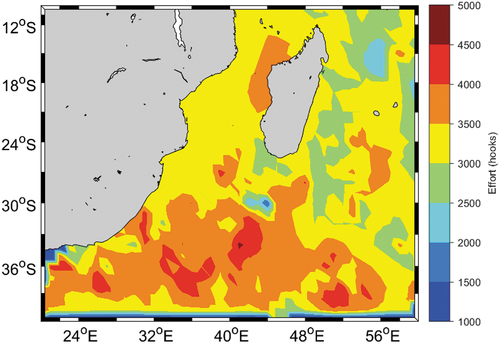
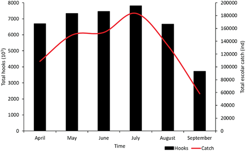
Escolar fishery data of Taiwanese tuna longline fishery in the Indian Ocean were collected from January 2010 to December 2014 supplied by the Overseas Fisheries Development Council of Taiwan. The monthly catch constantly showed an increase from February to July and gradually experienced a decrease from September to December for finding out the habitat suitability of escolar, we used the fishery data from April to September during 2010–2014 because these months were the peak fishing season of escolar (Figure 1). These data were 1º × 1º latitude and longitude. The fishing effort was spanned from 10 ºS-40 ºS and 20 ºE-60 ºE (Figure 2). The fishery data contained the number of hooks used, number of catches, year, latitude, and longitude. The stock abundance of escolar fish was determined by the Catch Per Unit Effort (CPUE) or called Nominal Catch Per Unit Effort (NCPUE) (Equation. 1) (Su et al. 2008; Vayghan et al. 2020).

(1) $CPU{E}_{ijk}=\sum C_{ijk}/\sum E_{ijk}$(1)

Figure 1. Total monthly catch trend of escolar in the southwestern Indian Ocean from 2014 to 2019.

Figure 2. The distribution of fishing effort of escolar for all vessels in the southwestern Indian Ocean between 2010 and 2014.

Where $C_{ijk}$ corresponds to the total catch with 1000 hooks, $E_{ijk}$ symbolizes the total fishing effort with 1000 hooks; i, j, and, k are symbolized the month, longitude, and latitude, respectively.

2.2. The standardization of Catch per Unit Effort (S.CPUE)

CPUE was standardized in order to remove accidentally biased estimation from fishery data with 1° grid data. NCPUE was standardized by using a generative linear model (GLM) in R (version 4.1.2), the computation of GLM equation as follows Equation (2)(2) $\begin{array}{rl}& \mathrm{l}\mathrm{o}\mathrm{g}\left(\mathrm{C}\mathrm{P}\mathrm{U}\mathrm{E}+\mathrm{c}\right)=\mathrm{Y}\mathrm{e}\mathrm{a}\mathrm{r}+\mathrm{M}\mathrm{o}\mathrm{n}\mathrm{t}\mathrm{h}+\mathrm{L}\mathrm{a}\mathrm{t}\mathrm{i}\mathrm{t}\mathrm{u}\mathrm{d}\mathrm{e}+\mathrm{L}\mathrm{o}\mathrm{n}\mathrm{g}\mathrm{i}\mathrm{t}\mathrm{u}\mathrm{d}\mathrm{e}+\mathrm{H}\mathrm{o}\mathrm{o}\mathrm{k}\mathrm{s}+\mathrm{I}\mathrm{n}\mathrm{t}\mathrm{e}\mathrm{r}\mathrm{a}\mathrm{c}\mathrm{t}\mathrm{i}\mathrm{o}\mathrm{n}\\ & \left(\mathrm{Y}\mathrm{e}\mathrm{a}\mathrm{r}\ast \mathrm{L}\mathrm{a}\mathrm{t}\mathrm{i}\mathrm{t}\mathrm{u}\mathrm{d}\mathrm{e}\right)+\text{isin}\end{array}$(2) (Su et al. 2008):

(2) $\begin{array}{rl}& \mathrm{l}\mathrm{o}\mathrm{g}\left(\mathrm{C}\mathrm{P}\mathrm{U}\mathrm{E}+\mathrm{c}\right)=\mathrm{Y}\mathrm{e}\mathrm{a}\mathrm{r}+\mathrm{M}\mathrm{o}\mathrm{n}\mathrm{t}\mathrm{h}+\mathrm{L}\mathrm{a}\mathrm{t}\mathrm{i}\mathrm{t}\mathrm{u}\mathrm{d}\mathrm{e}+\mathrm{L}\mathrm{o}\mathrm{n}\mathrm{g}\mathrm{i}\mathrm{t}\mathrm{u}\mathrm{d}\mathrm{e}+\mathrm{H}\mathrm{o}\mathrm{o}\mathrm{k}\mathrm{s}+\mathrm{I}\mathrm{n}\mathrm{t}\mathrm{e}\mathrm{r}\mathrm{a}\mathrm{c}\mathrm{t}\mathrm{i}\mathrm{o}\mathrm{n}\\ & \left(\mathrm{Y}\mathrm{e}\mathrm{a}\mathrm{r}\ast \mathrm{L}\mathrm{a}\mathrm{t}\mathrm{i}\mathrm{t}\mathrm{u}\mathrm{d}\mathrm{e}\right)+\text{isin}\end{array}$(2)

where CPUE indicates the nominal catch per unit effort, c is an indicator of the entire nominal catch mean used in the standardization with a constant value of 0.1, $\mu$ is the intercept and $\text{isin}$ is a variable of a normal distribution with zero means.

2.3. Remotely-sensed data

Ten remotely-sensing environmental data were compiled for environmental parameter selections from 2010 to 2014. The fishing data used in this study ranged from 2010 to 2014. To collect the required remote sensing data, we used the marine.copernicus.eu dataset, which covered the period 1993 to 2020. We chose a time frame of remote sensing data (2010–2014) that corresponded to the availability of fishing data within this dataset. This ensured that we had the required environmental data to match with the fishery records for our analysis. They were SSC, O, SST, SSH, Sea Surface Salinity (SSS), Mixed Layer Depth (MLD), eastward velocity (U), northward velocity (V), the potential of hydrogen (pH), and Eddie Kinetic Energy. EKE data were calculated according to Wang et al. (2017). These environmental parameters were selected for detecting the habitat suitability of escolar fish. Many studies have used them to understand the distribution, abundance, and prediction of fishes. SSH, SSS, SST, U, V, and MLD were collected from GLOBAL_REANALYSIS_PHY_001_031 product ID with spatial extent was categorized into global ocean Lat 80° to 90° Lon −180° to 180°, a fine resolution spatial grid ${0.25}^{\circ }\times {0.25}^{\circ }$, temporal extent 1 January 1993 to 15 December 2020, elevation (depth) levels 75, level 4 of processing, and all the parameters were daily data except MLD was monthly. These environmental data were retrieved in 2 May 2022. Meanwhile, O, pH, and SSC were collected from GLOBAL_REANALYSIS_BIO_001_029 product ID replaced with GLOBAL_MULTIYEAR_BGC_001_029 product ID with spatial extent was categorized into global ocean Lat −90° to 90° Lon −180° to 180°, a fine resolution spatial grid ${0.25}^{\circ }\times {0.25}^{\circ }$, temporal extent 1 January 1993 to 15 December 2020, elevation (depth) levels 75, level 4 of processing, and all the parameters were monthly data (Table 1). These environmental data were retrieved in 2 May 2022. All parameters were converted to the spatial resolution of fishery data (1° × 1º) by Matlab R(2019a).

Table 1. Remote sensing data resources and their description.

Parameter	Product ID	Spatial extent	Spatial resolution	Temporal extent	Elevation (depth) levels	Temporal resolution	Processing level
SSH	GLOBAL_REANALYSIS_PHY_001_031 https://data.marine.copernicus.eu/product/GLOBAL_REANALYSIS_PHY_001_031/description	Global Ocean Lat −80° to 90° Lon −180° to 180°	0.25° × 0.25°	1 January 1993 to 15 December 2020	75	Daily	4
SSS
SST
U
V
MLD						Monthly
O	GLOBAL_REANALYSIS_BIO_001_029 replaced with GLOBAL_MULTIYEAR_BGC_001_029 https://data.marine.copernicus.eu/product/GLOBAL_MULTIYEAR_BGC_001_029/description	Global Ocean Lat −90° to 90° Lon −180° to 180°	0.25° × 0.25°	1 January 1993 to 31 December 2020	75	Monthly
Ph
SSC

The environmental selections were conducted by GAM, RF, and BRT in R (version 4.1.2). The environmental parameters were selected according to R² that had more than 0.1 value for GAM, BRT, and RF for building model combinations to determine the preference environmental parameters of escolar in the southwestern Indian Ocean.

2.4. Suitability index curves of remotely-sensed variables

Suitability index (SI) curves indicate the relationship between each environmental variable and escolar. The optimal suitable habitat is considered SI > 0.6, and the equation of index is as follows (Equation (3) (Mondal et al. 2021; Vayghan et al. 2020).

(3) $\mathrm{S}\mathrm{I}=\frac{{\stackrel{\wedge }{\mathrm{Y}}}_{ijk}-{\stackrel{\wedge }{\mathrm{Y}}}_{ijkmin}}{{\stackrel{\wedge }{\mathrm{Y}}}_{ijkmax}-{\stackrel{\wedge }{\mathrm{Y}}}_{ijkmin}}$(3)

Where Ŷ indicates the predicted CPUE or remotely-sensed variables; Ŷ min and max indicate the minimum and maximum of remotely-sensed variables or CPUE prediction, i, j, and k denote the month, longitude, and latitude, respectively. For each environmental variable, SI scale ranges from 0 to 1, indicating the lowest suitable range to the highest range of environmental factors, respectively. SI curves were generated by calculating the SI value of each environmental variable as well as the midpoints of each class interval. Lastly, this below formula (Equation. 4) was used to calculate the combination of the selected environmental parameters and SI (Lee et al. 2020).

(4) $S{I}_m=e^{\alpha \left(m+\beta \right)2}$(4)

Where, m indicates the response variable, $\alpha and\beta$ is the least square estimate for minimizing the residual between the measured and estimated SI.

2.5. HSI model development

Two empirical HSI models, AMM and GMM, were used to analyse escolar fish habitat preference using the SI values of each environmental variable. The HSI value ranges from 0 to 1. The lowest value indicates unsuitability, while the highest value indicates suitability. The following formulas were used to calculate the HSI (Lee et al. 2020; Mondal et al. 2021).

(5) $HS{I}_{AMM=}\frac{1}{m}\sum _{n=1}^{m}S{I}_n$(5)

(6) $HS{I}_{GMM}={\left(\prod _{n=1}^{m}S{I}_n\right)}^{1/m}$(6)

Where, $S{I}_n$ indicates the SI for nth environmental parameters, and m denotes the number of environmental factors added into the model. In each empirical habitat model, the selected environmental parameter was used individually and together for habitat data. SI values higher than 0.6 were obtained through various habitat factor integrations and then integrated into the HSI model.

2.6. Model selection and validation of the HSI model

The selected environmental variables were combined to make combination models. The selected combination models were tested and validated by the lowest AIC. The lowest AIC indicates a good estimator to predict the accuracy (Abdul Azeez et al. 2021; Maydeu-Olivares and Garcia-Forero 2010). The model was considered the best-combined model to determine the habitat suitability of escolar fish. The correlation between S.CPUE and SI was evaluated for the prediction of habitat suitability of escolar fish in the southwestern Indian Ocean (Lee et al. 2020). Six-month data were analysed for predicting the spatial distribution of HSI values as aforementioned. Matlab R(2019a) was used to overlay the HSI model.

3. Results

3.1. The selection of the oceanographic parameters for model combinations

Ten environmental variables were evaluated for parameter selections as follows: SSC, O, SST, SSH, SSS, MLD, U, V, EKE, and pH according to R² value. Five out of ten environmental parameters were selected because R² that have more than 0.1 value to construct the environmental model combinations. The five parameters were SSC, O, SST, SSH, and SSS, among these five variables, SSC shows a higher R² in GAM (0.68), RF (0.38), and BRT (0.53) (Table 2).

Table 2. The selection of 10 environmental parameters by using GAM, RF, and BRT for constructing the model combinations.

	GAM				RF			BRT
Parameter	AIC	R^2	Dev. explained	DF	R^2	RMSE	MAE	R^2	RMSE	MAE
SSC	1553.41	0.68***	45.6	10.65	0.38***	0.86	0.52	0.53***	0.73	0.47
O	1663.62	0.62***	38.7	10.41	0.24***	0.97	0.62	0.41***	0.82	0.53
SST	1674.14	0.61***	37.9	9.51	0.23***	0.98	0.63	0.4***	0.82	0.53
SSH	1679.49	0.61***	37.6	10.60	0.21***	0.99	0.64	0.4***	0.82	0.54
SSS	1899.9	0.46***	20.5	10	0.05	1.14	0.75	0.23***	0.93	0.63
MLD	2048.09	0.06	5.78	3	0.01	1.18	0.82	0.09	1.01	0.73
U	2084.4	0.02	2.17	5.04	0	1.2	0.83	0.07	1.03	0.75
V	2085.16	0.02	2.42	8.16	0	1.22	0.85	0.06	1.03	0.76
EKE	2096.35	0.01	0.69	3.27	0	1.22	0.85	0.05	1.03	0.77
pH	2103.41	0	−0.11	3	0	1.23	0.86	0.04	1.04	0.77

Significant code: 0 ‘***’ 0.001 ‘**’ 0.01 ‘*’ 0.05 ‘.’ 0.1 ‘ ’ 1

3.2. NCPUE and S.CPUE

The temporal variability of NCPUE and S.CPUE show similar trends between 2010 and 2014 with fluctuating value. The year 2013 performed higher on both CPUE and S.CPUE and 2012 was lower (Figure 3). The analysed six-month data from April to September showed S.CPUE increased from April to July, however decreasing dramatically from August to September (Figure 4). Meanwhile, fishing effort was higher in 2013 and lower in 2012. July consistently exhibited higher fishing effort throughout all years, except in 2012, while September had the lowest fishing effort from 2010 to 2014 (Figure 5). According to the monthly pattern of hooks and escolar catches, it appears that the high catch depends on the fishing effort. When a greater number of hooks were utilized, the escolar catch was high from April to August. However, the catch declined when the fishing effort decreased (Figure 6).

Figure 3. The temporal variability of escolar fish in the southwestern Indian Ocean in 2010–2014.

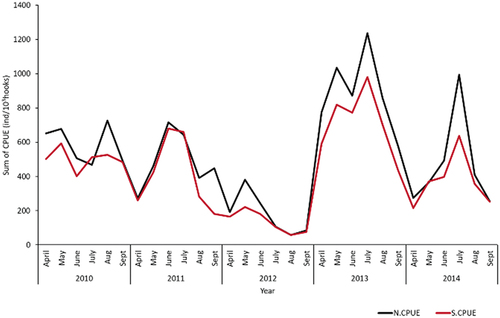
Figure 4. The averaged six analysed months (April–September) of N.CPUE and S.CPUE for escolar fish between 2010 and 2014.

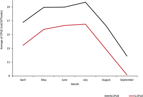
Figure 5. The sum of hooks used for escolar fish during fishing from 2010 to 2014 in the southwestern Indian Ocean.

Figure 6. Monthly hooks and escolar catch in the southwest Indian Ocean between 2010 and 2014.

3.3. SI curve

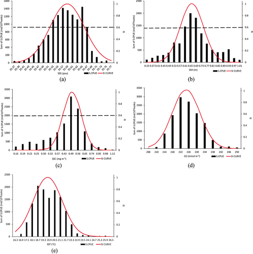
The escolar exhibited a preference for a specific range of environmental conditions. In terms of SSC, its optimal range was observed between 0.49 and 0.56 mg m⁻³, with a higher peak at 0.49 mg m⁻³. Likewise, the preferred O concentration was between 222 and 230 mmol m⁻³. Regarding SST, a slight variability of suitable habitat was identified within the range of 18.7–21.1°C, with a tendency towards the lower end at 18.7°C. SSH ranges between 0.61 and 0.69 m. SSS had a wider optimum range than other factors, ranging from 35.53 to 35.67 psu (practical salinity unit). Within this range, the higher peak was 35.65 psu. These findings highlight the specific environmental conditions that the escolar fish shows a preference for, emphasizing the importance of these factors in determining their suitable habitat (Figure 7).

Figure 7. SI curve of all environmental variables; (a) Sea Surface Salinity (SSS); (b) Sea Surface Height (SSH); (c) Sea Surface Chlorophyll (SSC); (d) Oxygen (O); and (e) Sea Surface Temperature (SST) for escolar fish in the southwestern Indian Ocean.

3.4. Model selection

A total of 29 model combinations were constructed using five parameters for the analysis, comparing AMM and GMM. The results indicate that AMM outperformed GMM in terms of its performance. The lowest AIC value of 28.49 was observed in AMM, specifically with a combination of SSH, SST, and O parameters. GMM, on the other hand, generated a higher AIC value of 31.25 using solely SSH and SST parameters (Table 2). These findings suggest that SSH, SST, and O are the most significant oceanographic factors for determining the habitat suitability of escolar in the southwestern Indian Ocean. The importance of these factors is further supported by the strong correlation between S.CPUE and SI for AMM, which was measured at R² 0.917 (Figure 8). This correlation validates that SSH, SST, and O play a crucial role in shaping the habitat preferences and distribution of escolar in the studied region.

Figure 8. The association between the number of hooks and escolar capture at a fishing ground in the southwestern Indian Ocean.

3.5. The spatial distribution and Predicted Habitat Suitability Index (PHSI)

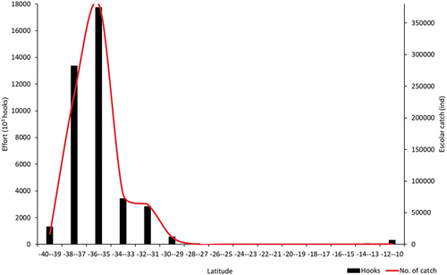
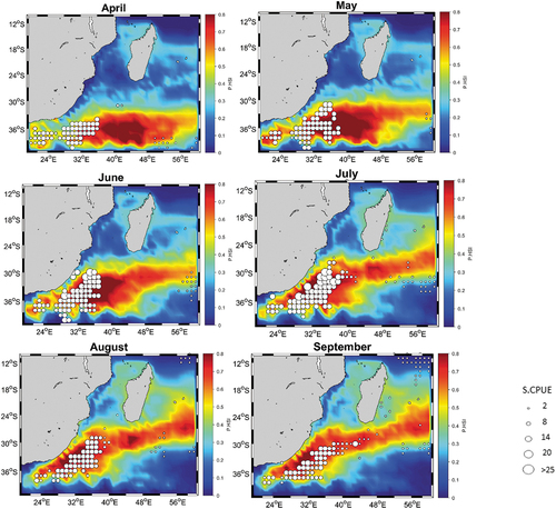
In June and July, a higher catch of escolar fish was observed, coinciding with their movement towards the northern part of the fishing ground from May to August. September, on the other hand, had the lowest escolar fish presence (Figure 10). The distribution of higher escolar fish concentrations was observed at coordinates 38 °S-30 °S and 28 °E-36 °E. Within this area, the fishing operation between 35 °S-38 °S exhibited both a high fishing effort and a high amount of escolar capture. In contrast, the fishing operation at 10 °S-34 °S experienced a significant decrease in activity (Figure 9). The presence of high escolar fish corresponds to with PHSI values greater than 0.6, indicating a favourable habitat. Moreover, the PHSI overlaid with the current catch distribution, emphasizing the areas where high escolar fish concentrations were found (Figure 10). These findings suggest that the observed high catch of escolar fish is likely due to their favourable habitat during the fishing period, in combination with the utilization of fishing efforts.

Figure 9. The association between S.CPUE of escolar and suitability index (SI) in the southwestern of Indian Ocean.

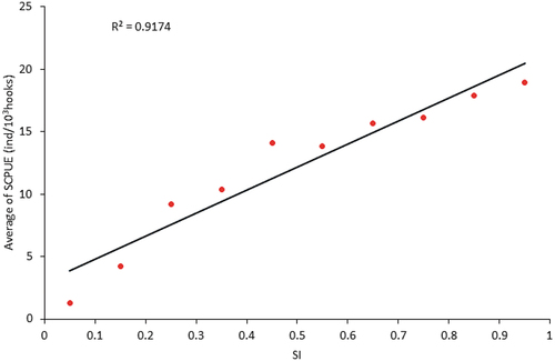
Figure 10. Spatial distribution of escolar fish in the southwestern Indian Ocean and the PHSI. The different sizes of circles in maps showed the average of S.CPUE, the smallest S.CPUE category was 2 and the highest was > 25.

4. Discussion

4.1. Time series

The abundance of escolar showed a significant increase in 2013 compared to a decrease in abundance in 2012 in the southwestern Indian Ocean (Figure 1). The high catch in 2013 can be linked to increased fishing effort during that time period (Figure 6). Fishermen are more likely to fish in areas with a high density of fish, frequently returning to the same fishing grounds as long as catch rates (measured in CPUE), remain high. If a high catch rate cannot be maintained and the catch rate falls to a level that would result in financial loss, fishermen prefer to move to area that can provide higher catch rates (Figure 2) (Li et al. 2014). The preference for fishing in locations with high concentrated fish populations is strongly influenced by the migratory routes of fish species. The seasonal movements and habitat distribution of fish are heavily influenced by oceanic conditions and the abundance of food resources (Hoolihan et al. 2014; Song et al. 2009). However, we did not determine immature and mature escolar to have better understanding either aggregate escolar in this fishing ground come for feeding or spawning ground. This is the limitation of this study. As a result, the spatio-temporal distribution of a fishing fleet should correspond to the suitable habitat or hotspots of fish (Li et al. 2014). Furthermore, the Indian Ocean has a strongly fluctuating environment so that it is possible that the favourable conditions at the time contributed to the abundant catch (Lumban-Gaol et al. 2021; Marsac 2006). This current study emphasizes the importance of three environmental factors, SSH, SST, and O, in shaping the distribution of escolar habitats, probably leading to the higher catch rates observed in the southwestern Indian Ocean (Table 3).

Table 3. The description of two HSI models – AMM and GMM with 29 environmental parameter combinations.

Model combination	AMM					GMM
	α (Intercept)	β	Adj R^2	DF	AIC	α (Intercept)	β	Adj R^2	DF	AIC
SSC+O	6.63	13.58	0.6	3	55.75	12.75	5.22	0.39	3	44.20
SSC+SSH	9.40	10.12	0.56		51.23	14.15	3.44	0.23		42.03
SSC+SST	6.11	14.03	0.78		48.18	12.50	5.63	0.42		44.44
SSC+SSS	8.27	10.88	0.62		50.54	12.62	5.58	0.43		44.20
O+SSH	6.07	13.66	0.73		44.81	10.55	7.23	0.75		32.41
O+SST	2.59	17.70	0.89		44.95	5	14.75	0.87		42.66
O+SSS	2.83	16.92	0.92		40.23	4.72	15.20	0.81		48.10
SSH+SST	6.11	13.90	0.83		44.60	10.13	8.59	0.88		31.25
SSH+SSS	8.36	10.26	0.81		40.26	10.63	7.95	0.79		36.18
SST+SSS	5.41	13.17	0.89		38.95	6.86	11.77	0.82		42.17
SSC+O+SSH	4.55	16.86	0.7		49.98	13.65	4.02	0.16		42.85
SSC+O+SST	2.25	19.40	0.8		48.08	12.37	5.89	0.29		44.63
SSC+O+SSS	2.25	19.40	0.8		48.08	12.11	6.42	0.4		42.80
SSC+SSH+SST	4.20	17.08	0.73		49.06	13.64	4.04	0.15		43.17
SSC+SSH+SSS	5.29	15.54	0.74		46.68	13.68	4.19	0.19		42.14
SSC+SST+SSS	4.37	15.67	0.85		41.09	12.22	5.94	0.33		43.70
O+SSH+SSS	3.76	16.49	0.86		41.39	10.01	8.67	0.74		36.45
O+SST+SSH	3.38	17.02	0.82		44.51	9.94	8.23	0.74		35.38
O+SSS+SST	1.50	18.32	0.89		40.21	4.62	15.14	0.82		36.45
SSH+SST+O	3.28	13.66	0.95		28.49	9.94	8.23	0.74		35.38
SSH+SST+SSS	4.52	15.46	0.92		37.86	9.62	9.25	0.87		33.83
SSH+SSS+O	3.61	16.95	0.91		41.83	9.80	9.35	0.85		35.71
SSC+O+SSH+SST	2.29	19.42	0.85		50.21	13.50	5.11	0.37		44.59
SSC+O+SSH+SSS	2.29	19.10	0.8		53.34	13.16	5.10	0.31		46.73
SSC+O+SST+SSS	0.98	20.13	0.85		50.90	11.72	6.81	0.46		47.15
SSC+SSH+SST+SSS	2.49	18.81	0.84		50.37	12.98	5.38	0.35		46.36
SSC+SSH+SSS+SST	2.49	18.81	0.84		50.37	12.98	5.38	0.35		46.36
SSH+SST+O+SSS	1.70	19.66	0.92		42.76	8.53	11.33	0.89		35.36
SSC+O+SSH+SST+SSS	1.27	20.45	0.88		48.97	12.49	6.35	0.38		48.37

bold numbers have 0 sig code

4.2. HSI model

HSI model performed AMM had lower AIC than GMM (Table 3). Other studies also showed AMM was the suitable model for the selection of the most suitable model and indicator (Lee et al. 2020; Yen et al. 2012). The outputs of empirical models were compared to the abundance density to assess their performance. It is critical to include both habitat characteristics and habitat selection in the interconnection between environmental features and target species’ habitat preferences when evaluating habitat suitability because an accurate HSI model can provide a reliable assessment. Uncertainty in HSI model prediction typically comes from three different sources. The first is the SI curve’s reliability. It is critical to obtain a reliable, single-variable SI curve representing species’ suitable environmental range is obtained. The second is the source of the input data representation. The distribution of variables in the study area must be reflected in the samples. As a result, the model can be examined and validated in order to optimize its goodness-of-fit for the HSI curve. The data collection can be boosted to minimize data input uncertainty. The third component is the HSI model structure. There is a significant difference between the outputs of various models. Information criterion such as AIC and Bayesian information Criterion can be used for best model selection. AIC is considered to have the advantage of testing the significance of differences in model specification’s functions (Chen et al. 2009; Van der Lee et al. 2006; Wang and Liu 2006).

4.3. Habitat preferences of escolar

Two phenomena occur in the Indian Ocean that influenced the number of fish biomass: positive and negative Indian Ocean Dipole (IOD) events that take place annually. During a positive IOD, upwelling and anomalies in Sea Surface Temperature (SST) occur, resulting in increased biological productivity and an abundance of food in location experiencing upwelling. This can cause a higher catch during fishing operation. Conversely, negative IOD events can lead to decreased fish populations due to downwelling, which results in lower biological productivity. Changes in temperature also impact biological production, thereby influencing fish behaviour and distribution (Lumban-Gaol et al. 2021). This correlation between negative IOD events and fish catch has also been observed in albacore studies which caused low catch in 2012 (Mondal et al. 2021). This finding aligns with the presence result with the lower catch rate observed in 2012 (Figure 3). Understanding of climate variability in this current fishing ground should be done in the future to investigate how IOD impacts on escolar catch at this sampling time frame.

Additionally, three environmental habitats were preferred by escolar were SST, SSH, and O (Table 3). A few studies have been done for determining whether SST is important for mesopelagic species such as yellowfin tuna, bigeye, Atlantic bluefin, and albacore tuna for influencing preying, diurnal migration, spawning, and reproduction (Alemany et al. 2010; Chen, Lee, and Tzeng 2005; Yang et al. 2020; Yen et al. 2012). SSH affects thermocline depth change which causes deeper thermocline (Liu et al. 2001). SSH has been previously linked to ocean current heat exchange. The convergence or divergence of ocean currents is caused by the rise and fall of sea level, which promotes bottom nutrient upwelling and so hence the fishery. Furthermore, the spatial distribution of fishing grounds had a strong relation to SSH (Wang et al. 2020). Oxygen is needed for metabolic, respiration, and swimming speed (Brill 1994). A study in the Caribbean found escolar spending in depths greater than 250 m and hours at night in shallower waters at 250 m depth that show a strong relationship between depth and temperature.

According to this present result, the oceanographic remote sensing data aforementioned performed their relation to spatial distribution and the predicted habitat suitability fit in the high distribution of escolar fish in the southwestern Indian Ocean (Figure 10). This indicates that satellite remote sensing is very powerful to gather data on oceanographic parameters. However, unavailable remote sensing dataset at particular time and location, and spatial temporal resolution of fishery data (1º) can be the limit of this method. Satellite oceanographic data can also be applied to create ecosystem indicators, regional ocean dynamics, ocean features, and larval transport (Tseng et al. 2010). Moreover, the detection habitat hot spot of albacore tuna was discovered by a multi-sensor satellite in the northwestern North Pacific. The hot spot habitat was associated with hydrographic features, frontal zones, and eddy fields so that distribution patterns and abundant tuna can be understood (Zainuddin et al. 2006).

4.4. Ecosystem-based fisheries management

Ecosystem-based fisheries management is crucial for the effective management of escolar in the southwestern Indian Ocean. The ultimate goal of ecosystem-based management in marine fisheries is to minimize the potential impacts of fishing activities while still allowing for sustainable fish extraction (Atkinson and Cools 2017). Escolar is commonly caught as bycatch by tuna longline fishing vessels operating in the Indian Ocean (Milessi and Defeo 2002). Given that the Indian Ocean is a significant supplier of commercial fisheries, particularly tuna, understanding the habitat requirements and distribution patterns of escolar becomes essential for improving fishery management and reducing unwanted escolar catch in the certain region. In order to reduce bycatch and ensure sustainable fishing practices, it is crucial to consider the environmental factors that influence escolar habitat conditions. By studying these factors, we can gain a better understanding of the relationship between environmental conditions and fish catch rates (Yen et al. 2012). This understanding forms an important foundation for implementing effective ecosystem-based fisheries management measures in the future. Furthermore, it is critical to recognize the influence of climate change on the marine environment, including rising temperatures, which can potentially alter fish habitat and distribution patterns. Therefore, it is imperative to evaluate and adapt climate change implementation in fisheries management strategies in the southwestern Indian Ocean to address the challenges posed by climate change (Bahri et al. 2021). In addition, understanding the spawning behaviour of escolar is essential. Promethichthys prometheus (Gempylidae) or roudi escolar starts the spawning time from April to September with the peak spawning season in June and July (Gonzalez-Pajuelo and Lorenzo Nespereira 1995). These months also coincide with high catch of escolar, especially in July (Figure 6) with the highest escolars were distributed at 30 ºS-36 ºS (Figure 10). This suggests that the identified area likely serves as a spawning or nursery habitat, emphasizing the need for its conservation to maintain escolar abundance. Considering the establishment of closed areas can help gain support for biodiversity conservation and protect critical spawning or nursery habitats (Van Overzee and Rijnsdorp 2015)

Furthermore, the conservation and sustainable use of marine resources align with the United Nations Sustainable Development Goal (SDG) 14, which aims to conserve and sustainably utilize oceans, seas, and marine resources (Virto 2018). As a top predator, escolar plays a crucial role in shaping marine food webs and responding to environmental changes (Hazen et al. 2019). Thus, managing the escolar fishery and protecting the marine ecosystem contribute directly to achieving SDG 14.

5. Conclusion

The AMM was determined to be the optimal model, having been selected based on three oceanographic parameters. The potential habitat of escolar fish in the southwestern Indian Ocean was showed to be influenced by SSH, SST, and O. The year 2013 exhibited a greater quantity of catch, whereas in all years, 2012 demonstrated a lesser amount of catch. The highest level of catch was observed in the month of July. This study suggested that the number of escolar catch are influenced by environmental conditions in the southwestern Indian Ocean. Thus, this information can be important to understand escolar fishery management.

Abbreviation words

AMM	=	Arithmetic Mean Model
GMM	=	Geometric Mean Model
GAM	=	Generalized Additive Model
BRT	=	Boosted Regression Trees
RF	=	Random Forest
AIC	=	Akaike Information Criterion
SI curve	=	Suitability Index curve
HSI model	=	Habitat Suitability Index model
CPUE/N.CPUE	=	Catch Per Unit Effort/Nominal Catch Per Unit Effort
S.CPUE	=	Standardized Catch Per Unit Effort
SSC	=	sea surface chlorophyll
O	=	Oxygen
SSS	=	Sea Surface Salinity
MLD	=	Mixed Layer Depth
U	=	eastward velocity
V	=	northward velocity
pH	=	the potential of hydrogen
EKE	=	Eddie Kinetic Energy
adj R2	=	adjusted R-squared
R2	=	R-squared
PHSI	=	Predicted Habitat Suitability Index

Acknowledgements

The authors thank the National Science and Technology Council of Taiwan for the funding. We thank the fishery agency of Taiwan for supplying the fishery data.

Disclosure statement

No potential conflict of interest was reported by the author(s).

Additional information

Funding

This research was funded by the Fisheries Agency, Council of Agriculture, Executive Yuan, Taiwan (112-2.31–03).

References

- Abdul Azeez, P., M. Raman, P. Rohit, L. Shenoy, A. K. Jaiswar, K. Mohammed Koya, and D. Damodaran. 2021. “Predicting Potential Fishing Grounds of Ribbonfish (Trichiurus lepturus) in the North-Eastern Arabian Sea, Using Remote Sensing Data.” International Journal of Remote Sensing 42 (1): 322–342. https://doi.org/10.1080/01431161.2020.1809025.
- Alemany, F., L. Quintanilla, P. Velez-Belchí, A. García, D. Cortés, J. Rodríguez, M. F. de Puelles, C. González-Pola, and J. López-Jurado. 2010. “Characterization of the Spawning Habitat of Atlantic Bluefin Tuna and Related Species in the Balearic Sea (Western Mediterranean).” Progress in Oceanography 86 (1–2): 21–38. https://doi.org/10.1016/j.pocean.2010.04.014.
- Atkinson, J., and L. Cools. 2017. “Sustainability of Capture Fisheries and SDG 14: Life Below Water.” Asian International Studies Review 18 (1): 23–50. https://doi.org/10.1163/2667078X-01801002.
- Bahri, T., M. Vasconcellos, D. J. Welch, J. Johnson, R. I. Perry, X. Ma, and R. Sharma, eds. 2021. Adaptive management of fisheries in response to climate change. FAO Fisheries and Aquaculture Technical Paper No. 667. Rome, FAO.
- Brendtro, K. S., J. R. McDowell, and J. E. Graves. 2008. “Population Genetic Structure of Escolar (Lepidocybium flavobrunneum).” Marine Biology 155 (1): 11–22. https://doi.org/10.1007/s00227-008-0997-9.
- Brill, R. W. 1994. “A Review of Temperature and Oxygen Tolerance Studies of Tunas Pertinent to Fisheries Oceanography, Movement Models and Stock Assessments.” Fisheries Oceanography 3 (3): 204–216. https://doi.org/10.1111/j.1365-2419.1994.tb00098.x.
- Chang, Y. J., C. L. Sun, Y. Chen, S. Z. Yeh, and G. Dinardo. 2012. “Habitat Suitability Analysis and Identification of Potential Fishing Grounds for Swordfish Xiphias gladius, in the South Atlantic Ocean.” International Journal of Remote Sensing 33 (23): 7523–7541. https://doi.org/10.1080/01431161.2012.685980.
- Chen, I. C., P. F. Lee, and W. N. Tzeng. 2005. “Distribution of Albacore (Thunnus alalunga) in the Indian Ocean and Its Relation to Environmental Factors.” Fisheries Oceanography 14 (1): 71–80. https://doi.org/10.1111/j.1365-2419.2004.00322.x.
- Chen, X., G. Li, B. Feng, and S. Tian. 2009. “Habitat Suitability Index of Chub Mackerel (Scomber japonicus) from July to September in the East China Sea.” Journal of Oceanography 65 (1): 93–102. https://doi.org/10.1007/s10872-009-0009-9.
- Feng, B., C. Xinjun, and X. Liuxiong. 2007. “Study on Distribution of Thunnus obesus in the Indian Ocean Based on Habitat Suitability Index.” jfc 31 (6): 805–812.
- Gonzalez-Pajuelo, J. M., and J. M. Lorenzo Nespereira. 1995. “Population Biology of the Roudi Escolar Promethichthys Prometheus (Gempylidae) off the Canary Islands.” Scientia Marina 59 (3–4): 235–240.
- Hazen, E. L., B. Abrahms, S. Brodie, G. Carroll, M. G. Jacox, M. S. Savoca, K. L. Scales, W. J. Sydeman, and S. J. Bograd. 2019. “Marine Top Predators as Climate and Ecosystem Sentinels.” Frontiers in Ecology and the Environment 17 (10): 565–574. https://doi.org/10.1002/fee.2125.
- Hoolihan, J. P., R. J. D. Wells, J. Luo, B. Falterman, E. D. Prince, and J. R. Rooker. 2014. “Vertical and Horizontal Movements of Yellowfin Tuna in the Gulf of Mexico.” Marine and Coastal Fisheries 6 (1): 211–222. https://doi.org/10.1080/19425120.2014.935900.
- Lee, M.-A., J.-S. Weng, K.-W. Lan, A. H. Vayghan, Y.-C. Wang, and J.-W. Chan. 2020. “Empirical Habitat Suitability Model for Immature Albacore Tuna in the North Pacific Ocean Obtained Using Multisatellite Remote Sensing Data.” International Journal of Remote Sensing 41 (15): 5819–5837. https://doi.org/10.1080/01431161.2019.1666317.
- Li, G., X. Chen, L. Lei, and W. Guan. 2014. “Distribution of Hotspots of Chub Mackerel Based on Remote-Sensing Data in Coastal Waters of China.” International Journal of Remote Sensing 35 (11–12): 4399–4421. https://doi.org/10.1080/01431161.2014.916057.
- Liu, Q., Y. Jia, P. Liu, Q. Wang, and P. C. Chu. 2001. “Seasonal and Intraseasonal Thermocline Variability in the Central South China Sea.” Geophysical Research Letters 28 (23): 4467–4470. https://doi.org/10.1029/2001GL013185.
- Lumban-Gaol, J., E. Siswanto, K. Mahapatra, N. M. N. Natih, I. W. Nurjaya, M. T. Hartanto, E. Maulana, L. Adrianto, H. A. Rachman, and T. Osawa. 2021. “Impact of the Strong Downwelling (Upwelling) on Small Pelagic Fish Production During the 2016 (2019) Negative (Positive) Indian Ocean Dipole Events in the Eastern Indian Ocean off Java.” Climate 9 (2): 29. https://doi.org/10.3390/cli9020029.
- Marsac, F. 2006. “Indices of Environmental Variability in the Indian Ocean 1970-2005.” 8th Session of the Working Party of Tropical Tuna IOTC-2006-WPTT–08.
- Massuti, E., S. Deudero, P. Sanchez, and B. Morales-Nin. 1998. “Diet and Feeding of Dolphin (Coryphaena hippurus) in Western Mediterranean Waters.” Bulletin of Marine Science 63 (2): 329–341.
- Maydeu-Olivares, A., and C. Garcia-Forero. 2010. “Goodness-Of-Fit Testing.” International Encyclopedia of Education 7 (1): 190–196.
- Milessi, A. C., and O. Defeo. 2002. “Long-Term Impact of Incidental Catches by Tuna Longlines: The Black Escolar (Lepidocybium flavobrunneum) of the Southwestern Atlantic Ocean.” Fisheries Research 58 (2): 203–213. https://doi.org/10.1016/S0165-7836(01)00365-4.
- Mondal, S., A. H. Vayghan, M. A. Lee, Y. C. Wang, and B. Semedi. 2021. “Habitat Suitability Modeling for the Feeding Ground of Immature Albacore in the Southern Indian Ocean Using Satellite-Derived Sea Surface Temperature and Chlorophyll Data.” Remote Sensing 13 (14): 2669. https://doi.org/10.3390/rs13142669.
- Nakamura, I., and N. V. Parin. 1993. “FAO Species Catalogue, Snake Mackerels and Cutlassfishes of the World (Families Gempylidae and Trichiuridae).” FAO 2 (125): 1–136.
- Polovina, J. J., and E. A. Howell. 2005. “Ecosystem Indicators Derived from Satellite Remotely Sensed Oceanographic Data for the North Pacific.” ICES Journal of Marine Science 62 (3): 319–327. https://doi.org/10.1016/j.icesjms.2004.07.031.
- Quigley, D. T. G., and K. Flannery. 2005. “First Record of Escolar Lepidocybium Flavobrunneum (Smith, 1849) (Pisces: Gempylidae) from Irish Waters, Together with a Review of NE Atlantic Records.” The Irish Naturalists’ Journal 28 (3): 128–130.
- Runcie, R. M., B. Muhling, E. L. Hazen, S. J. Bograd, T. Garfield, and G. DiNardo. 2019. “Environmental Associations of Pacific Bluefin Tuna (Thunnus orientalis) Catch in the California Current System.” Fisheries Oceanography 28 (4): 372–388. https://doi.org/10.1111/fog.12418.
- Song, L., J. Zhou, Y. Zhou, T. Nishida, W. Jiang, and J. Wang. 2009. “Environmental Preferences of Bigeye Tuna Thunnus obesus, in the Indian Ocean: An Application to a Longline Fishery.” Environmental Biology of Fishes 85 (2): 153–171. https://doi.org/10.1007/s10641-009-9474-7.
- Su, N.-J., S.-Z. Yeh, C.-L. Sun, A. E. Punt, Y. Chen, and S.-P. Wang. 2008. “Standardizing Catch and Effort Data of the Taiwanese Distant-Water Longline Fishery in the Western and Central Pacific Ocean for Bigeye Tuna, Thunnus Obesus.” Fisheries Research 90 (1–3): 235–246. https://doi.org/10.1016/j.fishres.2007.10.024.
- Tseng, C.-T., C.-L. Sun, S.-Z. Yeh, S.-C. Chen, and W.-C. Su. 2010. “Spatio-Temporal Distributions of Tuna Species and Potential Habitats in the Western and Central Pacific Ocean Derived from Multi-Satellite Data.” International Journal of Remote Sensing 31 (17–18): 4543–4558. https://doi.org/10.1080/01431161.2010.485220.
- Van der Lee, G. E., D. T. Van der Molen, H. F. Van den Boogaard, and H. Van der Klis. 2006. “Uncertainty Analysis of a Spatial Habitat Suitability Model and Implications for Ecological Management of Water Bodies.” Landscape Ecology 21 (7): 1019–1032. https://doi.org/10.1007/s10980-006-6587-7.
- Van Overzee, H. M., and A. D. Rijnsdorp. 2015. “Effects of Fishing During the Spawning Period: Implications for Sustainable Management.” Reviews in Fish Biology and Fisheries 25 (1): 65–83. https://doi.org/10.1007/s11160-014-9370-x.
- Vayghan, A. H., and M. A. Lee. 2022. “Hotspot Habitat Modeling of Skipjack Tuna (Katsuwonus pelamis) in the Indian Ocean by Using Multisatellite Remote Sensing.” Turkish Journal of Fisheries and Aquatic Sciences 22 (9): TRJFAS19107. https://doi.org/10.4194/TRJFAS19107.
- Vayghan, A. H., M.-A. Lee, J.-S. Weng, S. Mondal, C.-T. Lin, and Y.-C. Wang. 2020. “Multisatellite-Based Feeding Habitat Suitability Modeling of Albacore Tuna in the Southern Atlantic Ocean.” Remote Sensing 12 (16): 2515. https://doi.org/10.3390/rs12162515.
- Virto, L. R. 2018. “A Preliminary Assessment of the Indicators for Sustainable Development Goal (SDG) 14 'Conserve and Sustainably Use the Oceans, Seas and Marine Resources for Sustainable development'.” Marine Policy 98:47–57. https://doi.org/10.1016/j.marpol.2018.08.036.
- Wang, M., Y. Du, B. Qiu, X. Cheng, Y. Luo, X. Chen, and M. Feng. 2017. “Mechanism of Seasonal Eddy Kinetic Energy Variability in the Eastern Equatorial Pacific Ocean.” Journal of Geophysical Research: Oceans 122 (4): 3240–3252. https://doi.org/10.1002/2017JC012711.
- Wang, J., Y. Jiang, J. Zhang, X. Chen, and D. Kitazawa. 2020. “Catch per Unit Effort (CPUE) Standardization of Argentine Shortfin Squid (Illex argentinus) in the Southwest Atlantic Ocean Using a Habitat-Based Model.” International Journal of Remote Sensing 41 (24): 9309–9327. https://doi.org/10.1080/01431161.2020.1798550.
- Wang, Y., and Q. Liu. 2006. “Comparison of Akaike Information Criterion (AIC) and Bayesian Information Criterion (BIC) in Selection of Stock–Recruitment Relationships.” Fisheries Research 77 (2): 220–225. https://doi.org/10.1016/j.fishres.2005.08.011.
- Yang, S., L. Song, Y. Zhang, W. Fan, B. Zhang, Y. Dai, H. Zhang, S. Zhang, and Y. Wu. 2020. “The Potential Vertical Distribution of Bigeye Tuna (Thunnus obesus) and Its Influence on the Spatial Distribution of CPUEs in the Tropical Atlantic Ocean.” Journal of Ocean University of China 19 (3): 669–680. https://doi.org/10.1007/s11802-020-4264-0.
- Yen, K. W., H. J. Lu, Y. Chang, and M. A. Lee. 2012. “Using Remote-Sensing Data to Detect Habitat Suitability for Yellowfin Tuna in the Western and Central Pacific Ocean.” International Journal of Remote Sensing 33 (23): 7507–7522. https://doi.org/10.1080/01431161.2012.685973.
- Zainuddin, M., H. Kiyofuji, K. Saitoh, and S.-I. Saitoh. 2006. “Using Multi-Sensor Satellite Remote Sensing and Catch Data to Detect Ocean Hot Spots for Albacore (Thunnus alalunga) in the Northwestern North Pacific.” Deep Sea Research Part II: Topical Studies in Oceanography 53 (3–4): 419–431. https://doi.org/10.1016/j.dsr2.2006.01.007.
- Zajac, Z., B. Stith, A. C. Bowling, C. A. Langtimm, and E. D. Swain. 2015. “Evaluation of Habitat Suitability Index Models by Global Sensitivity and Uncertainty Analyses: A Case Study for Submerged Aquatic Vegetation.” Ecology and Evolution 5 (13): 2503–2517. https://doi.org/10.1002/ece3.1520.