Estimation of tropical forest aboveground biomass in Nepal using multiple remotely sensed data and deep learning

ABSTRACT

This study assessed the prediction accuracy of the forest aboveground biomass (AGB) model using remotely sensed data sources (i.e. airborne laser scanning (ALS), RapidEye, Landsat), and the combination of ALS with RapidEye/Landsat using parametric weighted least squares (WLS) regression. We also analysed the AGB model using random forests, extremely randomized trees, and deep learning stacked autoencoder (SAE) network from nonparametric statistics to compare the performance with WLS regression. We also compared the widths of the 95% confidence intervals for estimates of the mean AGB per unit area using the model-based estimator. The study site in the Terai Arc Landscape, Nepal, comprised 14 protected areas extending from the southern part of Nepal to India and encompassed mosaics of continuous dense forest and tall grassland. The ALS data provided the largest prediction accuracy (0.30–0.35 relative root mean squared error (rRMSE)), whereas RapidEye and Landsat had smaller prediction accuracies (0.48‒0.54 and 0.47‒0.55 rRMSE, respectively) for the estimation of AGB. The combined use of ALS and RapidEye predictors in the AGB model reduced the rRMSE and narrowed the confidence interval compared with ALS alone, but the improvements were minor. The SAE prediction technique provided the largest prediction accuracy, with inputs of combined ALS and RapidEye predictors that yielded an R² of 0.80, an rRMSE of 0.30, and a confidence interval of 176‒184 compared to other tested prediction techniques. The SAE prediction technique can become more powerful than other tested prediction techniques if properly adjusted and tuned for accurate forest AGB mapping applications. To our knowledge, this is the first study assessing the performance of the SAE in AGB modelling with a range of hyper-parameter values.

KEYWORDS:

• Aboveground biomass
• RapidEye
• Landsat
• hyper-parameter
• deep learning
• random forests

1. Introduction

Forest aboveground biomass (AGB) estimation is pivotal in several forestry-related activities, such as silviculture, environmental management, biodiversity conservation, and restoration (Araza et al. 2022; Duncanson et al. 2021). Forest AGB estimation is also directly linked to carbon sequestration and carbon storage and plays a key role in climate change mitigation. The importance of the accurate estimation of forest AGB has been highlighted in international activities such as reducing emissions from deforestation and forest degradation in developing countries (REDD+) (Latifi et al. 2015), and the challenges to the successful implementation of these initiatives have been shown to arise from the need for reporting forest AGB stocks (Næsset et al. 2016). Advancements in remote sensing (RS) technology have enabled more accurate and precise estimation of AGB stocks (Araza et al. 2022; Duncanson et al. 2021). Among all carbon pools, AGB is the most dynamic and variable, quickly reflecting management-related changes (Duncanson et al. 2021; Houghton, Hall, and Goetz 2009).

Enhanced tropical forest AGB estimates could provide crucial information for global carbon accounting since the degradation and deforestation of tropical forests account for 10% of the total anthropogenic carbon emissions (IPCC, MassonDelmotte et al. 2021). Also, tropical forests store approximately 55% of the total carbon (Pan et al. 2011; Urbazaev et al. 2018) and contribute to 70% of the total global forest carbon sink (Urbazaev et al. 2018). The Intergovernmental Panel on Climate Change (IPCC) encouraged countries to carry out inventories on greenhouse gas, and REDD+ reporting should provide an accurate estimate of forest AGB (Hou et al. 2013; Rana 2016; Xu et al. 2018; Xu, Hou, and Tokola 2012). In turn, this will contribute to global efforts to combat climate change and preserve the vital role that tropical forests play in maintaining the Earth’s carbon balance.

Forest AGB has traditionally been estimated using field inventory methods (such as national forest inventories (NFIs)), which are expensive and restricted in time and space. A combination of RS data and field-based surveys can offer a practical and cost-efficient alternative for forest AGB estimation (e.g. Urbazaev et al. 2018). In the recent decade, a number of RS-based studies have been conducted at local (Hou, Xu, and Tokola 2011), national (Rodríguez-Veiga et al. 2016), continental (Baccini et al. 2008), and intercontinental scales (Avitabile et al. 2016). Among the RS sources, three-dimensional airborne laser scanning (ALS) data have frequently been reported to achieve a larger prediction accuracy across various geographical units (e.g. at the national level) for reducing the cost of large-scale forest AGB inventories (see Næsset et al. 2016). The ALS technology is now acknowledged to be the state-of-the-art preference for the RS-based assessment of AGB in extremely dense tropical forests (Chan, Fung, and Wong 2021). The accuracy and precision of ALS-based AGB estimation have varied from model to model and from area to area (Chan, Fung, and Wong 2021; Xu et al. 2018), although the ALS prediction technique had a larger estimation error for tropical forests compared to other biomes, such as boreal forests (Rana et al. 2014). The coarse-resolution RS data (e.g. Landsat) may over- or underestimate AGB stock in dense mixed-species tropical forests, whereas fine-resolution RS data (e.g. ALS) can overcome this problem by providing an accurate and precise estimate of AGB stock (Chan, Fung, and Wong 2021).

AGB estimation using RapidEye data has been reported infrequently in the literature (but see Rana et al. 2014), although it has been claimed that a 5-metre pixel size with an additional red-edge band (0.69–0.73 µm) is potentially effective in tropical AGB estimation over time and space (Næsset et al. 2016). The RapidEye and Landsat optical data provide only limited information on forest structure in the vertical direction, and they do not provide cloud-free datasets on a large scale (Rana 2016). The use of ALS data overcame the cloud problem, although the availability of temporally and radiometrically corrected datasets at a large scale could be an issue (Abbas et al. 2020; Avitabile et al. 2012).

One approach to reducing the AGB estimation error could be the combined use of ALS and optical data, such as RapidEye and Landsat. This approach is reasonable because wall-to-wall AGB estimation using multiple sources of RS data, e.g. at the landscape level, have to meet even greater accuracy standards for AGB estimates over time and space as compared with single-source AGB estimates (Næsset et al. 2016). On the other hand, a number of issues need to be resolved, including the spatio-temporal variation and the unique profiles of individual sensors, i.e. differences in spectral and radiometric resolution depending on the data (Rana 2016). The integration of various remote sensing data sources, like ALS, RapidEye, and Landsat, holds promise for improving AGB estimation accuracy in tropical forests. By addressing the challenges and limitations of each data source, this approach could provide a more precise and cost-effective method for monitoring forest AGB and carbon stocks over time and space, ultimately contributing to better global carbon accounting.

Machine learning algorithms have become widespread as a substitute for the parametric approach (e.g. Ghosh and Behera 2021; Hudak et al. 2008; Niemi et al. 2015). Such algorithms (e.g. random forests (RF), Breiman (2001) can retain the variance structure of the predictions or estimates with respect to the field data (Dong et al. 2020; Verrelst et al. 2012) and effectively handle diverse environmental characteristics, achieving a reasonable prediction accuracy (Niemi et al. 2015; Zhang et al. 2019). These machine learning algorithms do not make assumptions about distributional characteristics for either auxiliary predictors (e.g. ALS metrics) or the predictors of interest (AGB) in the machine learning algorithms (e.g. Bousquet, Luxburg, and Ratsch 2004; Cao et al. 2018; Verrelst et al. 2012). However, they may produce a significant mean difference between observed and predicted values (LeMay and Temesgen 2005; Zhang et al. 2020).

Deep learning, a subset of machine learning techniques, excels at uncovering complex, nonlinear patterns in forest AGB (Zhang et al. 2019). It has also demonstrated the potential for classifying tree species, forest type, and land-use change detection (Nezami et al. 2020). Recently, the stacked autoencoder (SAE) network, a deep learning algorithm, has been employed for forest AGB estimation (Zhang et al. 2019) and image classification (Zhang, Ma, and Zhang 2016). The superior performance of the deep learning algorithm compared to the traditional parametric regression, other machine learning algorithms, e.g. RF and the extremely randomized trees (ERT) for AGB estimation, have been mentioned in some recent studies (Ayrey and Daniel 2018; Zhang et al. 2019). The combined use of ALS and RapidEye/Landsat predictors with the deep learning algorithms has the potential to reduce the estimation error compared to the other machine learning algorithms (Cao et al. 2018).

A plausible candidate model with a greater prediction accuracy may be deceptive if it is used to estimate population parameters or confidence intervals on data different from the ones used to fit the model (Hou et al. 2017). Confidence intervals for estimates of mean AGB per unit area depict the evaluation of the degree of accuracy of these products in geographical areas outside the calibration area (Baccini et al. 2012) or carbon policy development at various resolutions (Herold et al. 2019). Therefore, model comparisons of population estimation properties or confidence intervals are always preferred over-relying on prediction accuracy (Hou et al. 2017). In this paper, we compared the widths of the 95% confidence intervals for estimates of the mean AGB per unit area using the model-based estimator.

Our study assessed the prediction accuracy of the AGB model from RS data sources (i.e. ALS, RapidEye, Landsat) and the combination of ALS with RapidEye/Landsat using parametric multiple linear regression (weighted least squares, WLS). The study also analysed the AGB prediction techniques (ALS, RapidEye, Landsat, ALS+RapidEye, ALS+Landsat) using RF, ERT, and SAE from nonparametric statistics to compare the performance with WLS regression. The overall goal of this study was to improve the accuracy of AGB estimates using ALS and satellite imagery. The specific objectives were two-fold, namely 1) to select the optimum predictor variables among ALS, RapidEye, Landsat, and combinations of ALS and optical predictors; and 2) to select the optimum models to use with predictor variables to improve AGB estimates. To our knowledge, this is the first study to assess the performance of the SAE prediction technique in AGB modelling with a range of hyper-parameter values.

2. Materials and methods

2.1. Study area and experimental data

The study area is located in the Terai Arc Landscape (TAL) in southern Nepal (27.14°−29.08° N and 80.15°−85.49° E), as shown in Figure 1. The TAL area is a chain of 14 protected areas located in the southern part of Nepal, close to the boundary with India. It covers 23,000 km² and consists of a mosaic of patches of continuous dense forest. The region encompasses a flat plateau with an elevation range between 60 and 300 metres. The climate ranges from tropical to subtropical, with most tropical areas in the east and drier areas in the west. Typical precipitation ranges between 600 millimetres in the west and 1,300 millimetres in the east, with winter rain occurring in the west. A total of 22% of the country’s land area belongs to this zone (Rana 2016). Several ecosystem services are provided by the region, including those related to production, ecology, and protection, as well as sustainable livelihoods. The major tree species are Sal (Shorea robusta), Chir Pine (Pinus roxburghii), Marking Nut (Semecarpus anacardium), Axle Wood (Anogeissus latifolia), Schima (Schima wallichii), Karmal (Dillenia pentagyna), Java plum (Syzygium cumini). Other trees include Indian Gooseberry (Phyllanthus emblica), Indian Laurel (Terminalia tomentosa), and Malabar Plum (Syzygium jambos).

Figure 1. Map of the Terai Arc Landscape (TAL) area in Nepal and airborne laser scanning blocks.

The field sample data and RS data were compiled from previous studies in the same area (see Rana 2016; Rana et al. 2017). For more information on the datasets, see Rana (2016) and Rana et al. (2017). A total of 960 sample plots were initially designed, however, 632 sample plots (radius 12.5 m) were surveyed from March to May 2011 (Table 1). Systematic cluster sampling was used to place the sample plots within rectangular blocks. Each rectangular block (a size 5 km × 10 km) contained six clusters, with eight plots in each cluster. It is worth noting that there was none or a small spatial correlation between sample plots within the same cluster in the study area (Rana 2016; Tokola and Shrestha 1999), but observations and measurements might be correlated. A total of 328 plots were unmeasured or partially measured due to GPS positioning errors and inaccessibility. As a handheld GPS was difficult to use in mountainous Nepal with inaccessible conditions, such as steep slopes and dense forests, the positioning errors were included in the unmeasured or partially measured sample plots. The average AGB values were 302 tons/hectare for partly measured sample plots and 188 tons/hectare for fully measured sample plots. The species and diameter at breast height (DBH) of all trees with DBH ≥5 cm were assessed in each plot. Every 5^th tallied tree was measured in the plot and used to calibrate height models for estimating the heights of the remaining tally trees. The AGB values (tons/hectare) were estimated from tree-level attributes (e.g. height, DBH, species, wood density factor) using standard models and methods described in detail in Rana (2016).

Table 1. Forest attributes in the sample plots. SD − Standard deviation, DBH − Diameter at breast height and AGB −Aboveground biomass of all trees per hectare.

Forest attributes	Range	Mean±SD
Height (m)	5 − 47	17 ± 6
DBH (cm)	6 − 100	33 ± 16
Stem volume (m^3/hectare)	1 − 526	144 ± 97
AGB (tones/hectare)	1 − 675	183 ± 122

The ALS data were acquired between 14 March and 2 April 2011, using a Leica ALS50-II scanner. The ALS flight was operated at an altitude of 2,200 m above ground level, which yielded nominal ALS echoes with a density of 0.8/m². The ALS points were classified as ground and non-ground points following the methodology of Axelsson (2000). A 1 m digital terrain model (DTM) was created from the ground points, and the DTM was used to normalize the heights (z values) of the ALS points. A total of 12 RapidEye satellite image tiles, with a spatial resolution of 5 m consisting of five spectral bands, were acquired between 15 and 25 March, 2011. Radiometric and geometrical corrections were performed on the RapidEye images according to the RapidEye manual (RapidEye 2020). Four Landsat 5 TM satellite images were acquired in January 2010 and February 2011 and corrected radiometrically and geometrically. Multiple linear regression analyses were performed to calibrate Landsat images, as demonstrated by Tokola, Löfman, and Erkkilä (1999). Calibration was primarily concerned with the effects of sun sensor angle and atmospheric conditions (Tokola, Löfman, and Erkkilä 1999).

2.2. Predictors derived from the RS data

Predictors were extracted from the ALS data using the area-based approach (Cao et al. 2018; Latifi et al. 2015; Næsset 2002). A total of 30 ALS predictors related to the height and density of the ALS pulse returns were calculated from the first and last echoes. The above predictors have been used in other recent studies (e.g. Cao et al. 2018; Latifi et al. 2015; Rana 2016). First echoes comprised of echo categories ‘first of many’, and ‘only’ and last echoes comprised of ‘last of many’ and ‘only’. The first and last echoes contained most of the information about the upper and lower canopy (Hou, Xu, and Tokola 2011; Næsset et al. 2016; Rana 2016). The use of a threshold value for ALS predictor extraction was based on previous studies (see Kauranne et al. 2017; Rana et al. 2017). The ALS predictors were extracted using R and Python programming and were as follows:

• Height percentiles of first echoes at 10, 20, 30, … 100^th.

• Height percentiles of last echoes at 10, 20, 30, … 100^th.

• Mean height of first echoes over a threshold of 5 m.

• Standard deviation of first echo height.

• Proportion of first echoes less than 5 m to all first echoes.

• Proportion of last echoes less than 5 m to all last echoes.

• Proportion of last echoes with a height less than 1.5 m + i × 3 m for i = 0…7 and total number of last echoes.

• Logarithm of the first echo height less than 5 m to all first echo heights.

• Average height of the highest three echoes from the first echoes.

A total of 21 predictors from RapidEye data were extracted. The predictors were the means of the five spectral bands as well as a near-infrared-based normalized difference vegetation index (NIR NDVI) and a red-edge NDVI (Xie et al. 2018). In addition, NIR-based NDVI for individual sample plots was used to extract 14 textural predictors, namely angular second moment, contrast, correlation, sum of squares or variance, inverse difference moment, sum average, sum variance, entropy, sum entropy, difference variance, difference entropy, information measures of correlation, second information measures of correlation, and maximal correlation coefficient (Haralick, Dinstein, and Shanmugam 1973). We used the haralick function in the mahotas library in Python programming to extract the textural predictors. Textural features from NIR-based NDVI helped to describe the spatial distribution of biomass in the region of interest (Hou, Xu, and Tokola 2011; Rana 2016). In addition to calculating the mean values of the six Landsat TM bands, we also derived two vegetation indices, i.e. NDVI and atmospherically resistant vegetation index (ARVI, Kaufman and Tanre 1994). In total, eight Landsat predictors were used in building the AGB model. If the sample plot polygon boundary was covered in more than one raster pixel, the average value of raster pixels was used.

2.3. Development of the AGB model

The term ‘AGB model’ here refers to the combination of the mathematical expression representing the relationship between field-measured AGB and RS predictors. In the AGB model, RS predictors were compiled using a hybrid approach. First, a correlation filter (findCorrelation function, R Core Team 2020) was used to ensure that the multicollinearity among the predictors was minimized. A correlation filter refined the list of candidate predictors using a pair-wise correlation among the predictors. If two predictors had a correlation value greater than 0.8, the findCorrelation function excluded the predictor with the largest absolute mean correlation. An exhaustive search of the predictors using an efficient branch-and-bound algorithm was also performed. The regsubsets function in leaps packages was used, which applied the Bayesian Information Criterion (BIC) for selecting a subset of predictors (R Core Team 2020). In addition to the above steps, the maximum R² (coefficient of determination) improvement approach was used to select the RS predictors to be included in the models (Latifi et al. 2015; Næsset et al. 2016).

The AGB model was developed using WLS regression which was easy to understand and interpret the correlation between AGB and predictors derived from ALS/RapidEye/Landsat. The weights were constructed in such a way that the sample plot measurements with smaller variances were given greater weight. However, nonparametric statistics, i.e. RF, ERT, and SAE prediction techniques, were also used individually in building the AGB model. The AGB models from these two families (i.e. parametric and nonparametric statistics) may behave quite differently (Hou, Xu, and Tokola 2011; Latifi and Koch 2012; Zhang et al. 2019), and it was crucial to assess how the estimation error varies from parametric WLS regression to deep learning SAE.

The RF makes final decisions using ensemble decision trees based on a majority vote (Breiman 2001). The parameters used in the RF were 501 decision trees (ntree), three predictors at each split (mtry), and 100 times iterations. We validated these parameter choices through a series of cross-validation experiments, in which we systematically varied the parameters and evaluated the performance of the resulting models. The chosen configuration delivered the best balance of predictive accuracy and model complexity in these experiments. The ERT is similar in manner to RF but reduces the variance and the mean difference by increasing randomization and using the whole original sample rather than bootstrap replicas (Geurts, Ernst, and Wehenkel 2006). While splitting a tree node, the ERT randomly chooses both attributes and cut-points (Geurts, Ernst, and Wehenkel 2006). As with the RF, ntry = 501 and mtry = 3 were used (Table 2).

Table 2. Hyperparameter range and optimal value for each machine learning algorithm.

Algorithm	Hyperparameter ID	Range	Optimal value
RF	mtry	1 − 5	3
	ntree	2 − 1000	501
ERT	mtry	1 − 5	3
	ntree	2 − 1000	501
	numRandomCuts	1 − 10	3
SAE	hidden layers	1 − 3	2
	neurons	list(c(32,16), c(64,32), c(128,64), c(264,128))	c(264,128)
	activation	Tanh, Rectifier	Tanh
	learning rate	c(0.01,0.02)	0.01
	input dropout ratio	c(0,0.2,0.4,0.5)	0.2
	rate decay	c(1e-4, 3e-4, 6e-4)	6e-4
	momentum start	c(0.1,0.2)	0.1
	momentum stable	c(0.3,0.5,0.7)	0.5
	L1 (lasso) regularization	seq(0,1e-4,1e-6)	1e-4
	L2 (ridge) regularization	seq(0,1e-4,1e-6)	1e-5
	Loss function	Absolute, Quadratic, Huber,	Huber

The SAE, a deep learning algorithm, was used in AGB model development. It automatically extracts features through multiple layers of nonlinear processing to make them flexible in modelling the complex relationships with AGB compared to the classical prediction techniques (i.e. WLS) (Shao, Zhang, and Wang 2017). The SAE uses a hierarchical approach to build a deep neural network to extract deep features of data; it has an encoder and a decoder. An encoder converts the RS predictors into digital signals, whereas a decoder reconstructs the RS predictors from the digital signals. After each autoencoder is trained and after discarding the decoding layers, an SAE is formed using the encoder to all SAEs in a predictor-by-predictor manner (i.e. stacked). Subsequently, a deep neural network uses these trained SAEs to implement the AGB prediction work. Here, the grid search function of the R program was used to find the optimum value for different parameters of SAE (Table 2). The data were normalized using minimum and maximum values derived from training data to allow the SAE prediction technique to reconstruct the data effectively. Two convolutional layers with 264 and 128 nodes, respectively, were used. Each layer’s output was standardized and passed through an activation function based on the Hyperbolic tangent function (Tanh). An activation function indicates the contribution of the input from the previous layer to the final output. A dropout layer with a rate of 0.2 was used to prevent overfitting and enhance the generalization ability of the network. The dropout rate of 0.2 means 20% of the hidden features were dropped randomly. The initial learning rate of 0.01 with a momentum of 0.5, a rate decay of 0.0006, L1 (Lasso) regularization of 0.0001, and L2 (Ridge) regularization of 0.00001, was used to optimize the SAE network parameters. The SAE used the Huber loss function (Equations 1(1) $L_{HUBER}=\left\{\begin{array}{c}\frac{1}{2}||P^{\left(j\right)}-O^{\left(j\right)}||\begin{array}{c}2\\ 2\end{array}for||P^{\left(j\right)}-{O^{\left(j\right)}||}_1\le 1,\\ ||P^{\left(j\right)}-{O^{\left(j\right)}||}_1-\frac{1}{2}otherwise\end{array}\right.$(1) , L_HUBER) to optimize the learning curve of the AGB model. As a result of the prediction of the final layer, the loss was calculated using the difference between the predicted and observed AGB value:

(1) $L_{HUBER}=\left\{\begin{array}{c}\frac{1}{2}||P^{\left(j\right)}-O^{\left(j\right)}||\begin{array}{c}2\\ 2\end{array}for||P^{\left(j\right)}-{O^{\left(j\right)}||}_1\le 1,\\ ||P^{\left(j\right)}-{O^{\left(j\right)}||}_1-\frac{1}{2}otherwise\end{array}\right.$(1)

where P and O indicate the predicted and observed values for the training example of j, respectively. The SAE was trained over 60 epochs, using a batch size of 10. Nonetheless, to prevent model overfitting, an early stop was used with a patience value of five. This means that if accuracy was not improved (i.e. root mean square error, RMSE) after five iterations, the process would end. The R packages randomForest function from random forests, extraTrees function from extra trees, and h2o.deeplearning function from H2O were used to implement the RF, ERT, and SAE, respectively (R Core Team 2020).

A total of 20 AGB models were developed using WLS, RF, ERT, and SAE from the (i) ALS, (ii) RapidEye, (iii) Landsat, (iv) ALS + RapidEye, and (v) ALS + Landsat, respectively. We presented the width of the confidence intervals (95%) for estimates of the mean AGB per unit area. We used the model-based estimator given in Equation (2)(2) $\hat{\mu }=\frac{1}{K}\sum _{k=1}^K{\hat{y}}_k$(2) , variance (Equation 3(3) $$\widehat{Var}\left(\widehat{\mu }\right)=\frac{1}{K-1}{{\displaystyle \sum _{k=1}^k\left({\widehat{\mu }}^{°}-{\widehat{\mu }}_k^{°}\right)}}^2$$(3) ), and bootstrapping resampling (random) to report the width of the confidence intervals for estimates of the mean AGB per unit area. During the bootstrapping resampling procedure, we used bootstrapping residuals and cluster bootstrapping (Efron and Tibshirani 1994; Field and Welsh 2007). With this approach, we focused on resampling the residual errors and draws a random cluster from N (0,${\hat{\mathrm{\Sigma }}}_{K\times K}$) and adding them back to the prediction techniques to form a resample or bootstrap cluster resample. During the cluster sampling, we used single-stage cluster sampling, which consists of first randomly selecting clusters and then selecting all plots within clusters. With this approach, we retained the spatial structure of the sample data and mimicked the original sampling design. We resampled the original calibration size 632 plots 10,000 times with replacements. Rather than the number of resampling, the most important issue is whether the estimates remained stable. For this study, 10000 repetitions were sufficient because the estimates changed little after 8,000 repetitions.

(2) $\hat{\mu }=\frac{1}{K}\sum _{k=1}^K{\hat{y}}_k$(2)

(3) $$\widehat{Var}\left(\widehat{\mu }\right)=\frac{1}{K-1}{{\displaystyle \sum _{k=1}^k\left({\widehat{\mu }}^{°}-{\widehat{\mu }}_k^{°}\right)}}^2$$(3)

where $\hat{\mu }$ is the mean AGB ($\hat{y}$), $\widehat{Var}\left(\hat{\mu }\right)$ is the variance of AGB, $$\widehat{\mu }°=\frac{1}{K}{\displaystyle \sum _{k=1}^k{\widehat{\mu }}_k^{°}}$$, and $${\widehat{\mu }}_k^{°}$$ is the bootstrap estimate. We used 10,000 (k = 1, … ., K) iterations for bootstrapping resampling. The variable importance function in respective prediction techniques (i.e. WLS, RF, ERT, and SAE) was used to identify the relative importance of various predictors of ALS/RapidEye/Landsat for each AGB model. Each model’s performance was evaluated using RMSE (Equation 4), relative RMSE (rRMSE, Equation 4), MD (mean difference), and R². Using 632 plots, 10-fold cross-validation was employed and repeated 10 times, and the average values were reported in the results (Cao et al. 2018; Chan, Fung, and Wong 2021).

$RMSE\hspace{0.17em}=\sqrt{\frac{{\sum }_{\mathrm{i}=1}^{\mathrm{n}}{\left(\hspace{0.17em}{\mathrm{y}}_{\mathrm{i}}-{\hat{\mathrm{y}}}_{\mathrm{i}}\right)}^2}{\mathrm{n}}}$, $rRMSE\hspace{0.17em}=\frac{\mathrm{R}\mathrm{M}\mathrm{S}\mathrm{E}}{\bar{\mathrm{y}}}$ (4)

where $y_{\mathrm{i}}$ represents the observed value for a specific sample plot and $\widehat{y_i}$ represents the estimated value for the same sample plot i, $\bar{y}$ represents the mean value of the observed sample plots, and n signifies the total count of sample plots.

3. Results

3.1. Relationship between AGB and RS predictors

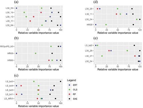
ALS (n = 5, Figure 2), RapidEye (n = 3, Figure 3), and Landsat (n = 5, Figure 4) predictors were statistically significantly correlated with AGB (Spearman’s correlation coefficient, p < 0.05). The importance assigned to different predictors varied among estimation methods (Figure 5). As a result, ERT indicated that some predictors were more important compared to others. A noteworthy finding was that the importance assigned by SAE to each predictor was homogenous (relative importance values of the predictors were similar). In the ALS prediction technique, height values at the 40^th percentile of the first echoes had a larger importance value compared to other predictors. In the combined approaches (ALS + RapidEye, ALS + Landsat), ALS predictors had more importance compared to RapidEye/Landsat predictors (Figure 5).

Figure 2. Correlation between ALS predictors, i.e., (a) L30_04: height values at the 40^th percentile of first echoes, (b) L30_11: height values at the 10^th percentile of last echoes, (c) L30_15: height values at the 50^th percentile of last echoes, (d) L30_16: height values at the 60^th percentile of last echoes, (e) L30_29: density values of the first echoes (between 1 and 5 m), and AGB: aboveground biomass. r: Spearman’s correlation coefficient with a significance level (or p-value) of the correlation.

Figure 3. Correlation between RapidEye predictors, i.e., (a) RE5pcPS_b3: red band means value, (b) HR06: sum average, (c) HR08: sum entropy, and AGB: aboveground biomass. r: Spearman’s correlation coefficient with a significance level (or p-value) of the correlation.

Figure 4. Correlation between Landsat predictors, i.e., (a) LS_bd1: blue band means value, (b) LS_bd3: red band means value, (c) LS_bd4: near-infrared band means value, (d) LS_bd5: short-wave infrared band means value, (e) LS_ARVI: atmospherically resistant vegetation index, and AGB: aboveground biomass. r: Spearman’s correlation coefficient with a significance level (or p-value) of the correlation.

Figure 5. Relative variable importance value used to train weighted least squares (WLS), random forests (RF), extremely randomized trees (ERT), and stacked autoencoder (SAE) prediction techniques for ALS (a), RapidEye (b), Landsat (c), ALS+RapidEye (d), and ALS+Landsat (e). Variable importance values represent the contribution of each variable in the prediction of forest aboveground biomass (AGB). L30_04: height values at the 40^th percentile of first echoes, L30_11: height values at the 10^th percentile of last echoes, L30_15: height values at the 50^th percentile of last echoes, L30_16: height values at the 60^th percentile of last echoes, L30_29: density values of the first echoes (between 1 and 5 m). RE5pcPS_b3: RapidEye red band mean value, HR06: RapidEye sum average, HR08: RapidEye sum entropy, LS_bd1: Landsat blue band mean value, LS_bd3: Landsat red band mean value, LS_bd4: Landsat near-infrared band mean value, LS_bd5: Landsat short-wave infrared band mean value, LS_ARVI: Landsat atmospherically resistant vegetation index.

3.2. AGB model development using WLS

The ALS prediction technique consisted of five predictors related to tree height and density (Table 3). Though both the first and last echoes of ALS data were used to form models, the first echoes had a more correlation with AGB compared to the last echoes (Table 3, Figure 2). It would not have been accurate to form AGB models using only the first echoes as they were mainly derived from the upper canopy (Næsset et al. 2016). For the RapidEye prediction technique, the mean value of the red band and the sum of averages accounted for much more of the variability in AGB than the sum of entropy (Table 3, Figure 3). The model statistics showed that NIR and ARVI explained more of the variability in AGB than the other Landsat predictors (Table 3, Figure 4). Four predictors were used for the combined use of ALS and RapidEye, although three predictors from ALS had explained most of the variability in AGB (Table 3, Figure 2). In the second combined approach to the ALS and Landsat data in the AGB modelling, four predictors were used. Similarly, most of the predictors were derived from ALS data with a significant relationship (Spearman’s correlation coefficient, p < 0.05) with AGB (Table 3, Figure 2).

Table 3. Construction of AGB models for ALS, RapidEye, Landsat, ALS + RapidEye, ALS + Landsat using WLS regression.

Prediction techniques	Predictors	Estimate	Std. Error	t Value	Pr(>|t|)
ALS	(Intercept)	35.5	8.6	4.1	***
	Height values at the 40th percentile of first echoes	11.5	0.8	13.6	***
	Height values at the 10th percentile of last echoes	6.4	0.9	6.1	***
	Height values at the 50th percentile of last echoes	−5.7	2.1	2.9	*
	Height values at the 60th percentile of last echoes	4.8	1.9	4.8	*
	Density values of the first echoes (between 1 to 5 m)	−59.0	9.2	−6.0	***
RapidEye	(Intercept)	178.5	28.1	6.4	***
	Red band	0.1	0.1	−7.0	***
	Sum average	7.7	1.0	7.0	***
	Sum entropy	−41.6	9.3	−4.4	***
Landsat	(Intercept)	105.9	36.1	2.9	**
	Blue band	−0.5	0.1	−4.3	***
	Red band	1.0	0.2	4.2	***
	Near infrared band	−0.3	0.1	−4.2	***
	Short-wave infrared band	−0.1	0.1	−4.2	***
	Atmospherically resistant vegetation index	6014.1	1272.0	4.7	***
ALS + RapidEye	(Intercept)	39.8	13.7	1.9	.
	Height values at the 40th percentile of first echoes	10.9	0.67	16.2	***
	Height values at the 10th percentile of last echoes	5.3	1.0	5.3	***
	Density values of the first echoes (between 1 to 5 m)	−49.7	11.6	−4.3	***
	Sum average	0.8	0.5	1.5	.
ALS + Landsat	(Intercept)	39.8	10.8	3.6	***
	Height values at the 40th percentile of first echoes	12.0	1.0	11.6	***
	Mean height of all first echoes above 5 m	1.7	1.1	1.5	.
	Density values of the first echoes (between 1 to 5 m)	−71.7	11.1	−4.4	***
	Green band	0.1	0.1	0.7	.

Note: Significance codes: 0 ‘***’ 0.001 ‘**’ 0.01 ‘*’ 0.05 ‘’. 0.1 ‘’ 1.

In the comparison of individual sensor results, the ALS prediction technique yielded the smallest estimation error, followed by RapidEye and Landsat (Table 4, Figure 6). Correspondingly, the rRMSE of the ALS prediction technique was 0.35, followed by RapidEye’s 0.54 and Landsat’s 0.55. The ALS prediction technique data had the smallest AIC value compared to the other tested prediction techniques (Table 4).

Figure 6. Field-observed versus model-predicted (fitted) AGB using WLS regression. The regression line is presented in blue colour. rRMSE – relative root mean square error, MD − mean difference, and R² – Adjusted coefficient of determination.

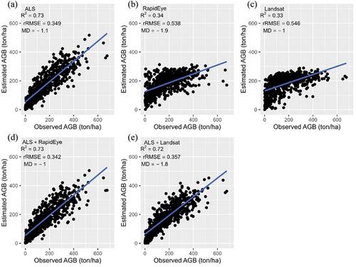
Table 4. Accuracy of the AGB models based on ALS, RapidEye, Landsat, ALS + RapidEye, and ALS + Landsat using WLS regression. rRMSE – relative root mean square error, MD − mean difference, Adj. R² – adjusted coefficient of determination, AIC−Akaike information criterion.

Prediction techniques	RMSE	rRMSE	MD	Adj. R^2	AIC	95% confidence interval bound lower – upper
ALS	62.9	0.349	−1.1	0.73	5622	17.0–194.5
RapidEye	98.0	0.538	−1.9	0.34	6111	167.8–195.1
Landsat	99.7	0.546	−1.0	0.33	6130	164.8–199.4
ALS + RapidEye	62.4	0.342	−1.0	0.73	5613	171.4–19.0
ALS + Landsat	65.3	0.357	−1.8	0.72	5632	171.6–19.3

The best performing was put in bold.

In the combined approach to the ALS predictors with RapidEye/Landsat predictors, the use of ALS and RapidEye predictors in the AGB model reduced the rRMSE by 0.007 compared with ALS alone but the improvements were minor (Cao et al. 2018; Hou, Xu, and Tokola 2011). The combined use of ALS and RapidEye predictors in the AGB model provided narrower confidence intervals compared to the other tested AGB models.

3.3. AGB model development using RF, ERT, and SAE

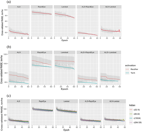
The same predictors (Table 3) were used for building the AGB model applying RF, ERT, and SAE prediction techniques to compare the performance with WLS regression. The hyper-parameter values in the SAE prediction technique affected the AGB model. The performances of few of the important hyperparameters, such as epoch, activation function, and the number of nodes in the hidden layer, are presented in Figure 7. The learning curves of the SAE were stable with the 60 epochs (Figure 7), and the Tanh activation function provided a smaller RMSE than Rectifier (Figure 7). Two hidden layers, with 264 and 128 per layer, provided the optimum result for the AGB model (Figure 7).

Figure 7. Learning curves (a), activation function (b) and nodes in hidden layers (c) of the SAE prediction technique based on the five sets of predictor variables, i.e. ALS, RapidEye, Landsat, ALS+RapidEye, and ALS+Landsat. Solid lines indicate the mean RMSE values, whereas the bounds of the shaded area indicate the minimum and maximum RMSE value per epoch. Each SAE prediction technique was cross-validated 10 times.

The SAE prediction technique provided a smaller rRMSE, followed by the ERT and the RF prediction techniques (Table 5). The RF and ERT prediction techniques, in most cases, produced similar prediction accuracies (i.e. R² and rRMSE values) in AGB estimation (Figures 8 and 9). Furthermore, the prediction accuracy was not necessarily increased by adding variables from RapidEye and Landsat, i.e. the prediction techniques with input of ALS predictors, in most cases, achieved smaller estimation errors than those with ALS+RapidEye and/or ALS+Landsat. The SAE prediction technique with ALS and RapidEye predictors provided the largest R² of 0.80 and the lowest rRMSE of 0.30 (Figure 10). Similarly, the combined use of ALS and RapidEye predictors in the SAE prediction technique provided narrower confidence intervals compared to the other tested prediction techniques.

Figure 8. Field-observed versus model-predicted (fitted) AGB using random forests. The regression line is presented in blue colour. rRMSE – relative root mean square error, MD − mean difference, and R² – Adjusted coefficient of determination.

Figure 9. Field-observed versus model-predicted (fitted) AGB using extremely randomized trees. The regression line is presented in blue colour. rRMSE – relative root mean square error, MD − mean difference, and R² – Adjusted coefficient of determination.

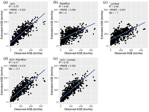
Figure 10. Field-observed versus model-predicted (fitted) AGB using stacked autoencoder. The regression line is presented in blue colour. rRMSE – relative root mean square error, MD − mean difference, and R² – Adjusted coefficient of determination.

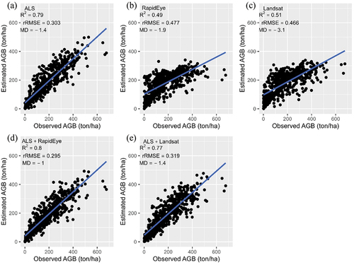
Table 5. Performance of RF, ERT and SAE prediction techniques for AGB estimation. rRMSE – relative root mean square error, MD − mean difference, and Adj. R² – adjusted coefficient of determination.

Prediction techniques		RMSE	rRMSE	MD	Adj. R^2	95% confidence interval bound lower – upper
RF	ALS	61.72	0.337	−0.3	.74	164.5–188.9
	RapidEye	88.42	0.484	−0.2	0.47	166.6–193.3
	Landsat	87.14	0.477	−0.4	0.48	163.9–196.6
	ALS + RapidEye	58.49	0.320	−0.8	0.77	173.5–191.2
	ALS + Landsat	59.53	0.325	−0.2	0.76	171.1–189.1
ERT	ALS	60.84	0.333	0.0	.75	170.2–193.3
	RapidEye	91.2	0.499	0.0	0.43	168.2–194.5
	Landsat	89.83	0.491	−1.0	0.45	165.8–197.8
	ALS + RapidEye	57.80	0.316	−0.7	0.77	173.8–19.4
	ALS + Landsat	59.13	0.323	0.1	0.76	171.5–189.5
SAE	ALS	55.36	0.303	−1.4	.79	176.2–187.3
	RapidEye	87.17	0.477	−1.9	0.49	174.2–187.3
	Landsat	85.23	0.466	−3.1	0.51	171.6–187.0
	ALS + RapidEye	54.01	0.295	−1.0	0.80	176.0–184.7
	ALS + Landsat	58.33	0.319	−1.4	0.77	177.9–187.3

The best performing was put in bold.

4. Discussion

This study considered the prediction accuracy of individual sensor results and the combination of ALS, RapidEye, and Landsat datasets for the estimation of AGB in a dense tropical forest in Nepal. As hypothesized, the ALS prediction technique provided smaller estimation errors in the AGB estimates than the RapidEye or Landsat prediction technique. Deep learning algorithms have recently attracted attention in forest inventory (e.g. Zhang et al. 2019), although many other fields, e.g. image classification and object detection, use deep learning algorithms extensively (Zhang, Ma, and Zhang 2016). This study showed the performance of the SAE prediction technique with a range of hyper-parameter values, which was our novelty compared to an earlier study by Zhang et al. (2019). The advantage of the SAE prediction technique is the automated learning of features. The SAE compresses the input feature (predictors) into a smaller-dimensional feature space and then estimates AGB from this representation. Deep learning algorithms provided smaller estimation errors compared to the nonlinear regression for forest attributes inventory (e.g. Ercanli 2020; Muukkonen and Heiskanen 2005; Ogana and Ercanli 2022; Ozcelik et al. 2013). Furthermore, the ERT prediction technique provided a slightly smaller RMSE than RF (e.g. Barrett et al. 2014). However, some studies, e.g. Latifi and Koch (2012), reported a smaller estimation error of RF over ERT in estimating forest AGB.

Several hyper-parameters influenced the performance of SAE prediction techniques, such as the number of nodes in the hidden layers, epochs, the activation function (result shown), input dropout ratio, and regularization parameters (result not shown) (Ghosh and Behera 2021; Lv et al. 2021; Ogana and Ercanli 2022). Interestingly, the Tanh activation function provided a smaller RMSE than the Rectifier activation function, although it is the default option for many SAE prediction techniques. A probable explanation could be that with Tanh activation, the nodes can learn more complex structures of AGB distribution in the study area (Bengio 2012; Heaton 2008; LeCun et al. 2012). The SAE prediction technique can become more powerful than other tested prediction techniques if properly adjusted and tuned for application in precision forest AGB mapping (Shao, Zhang, and Wang 2017; Zhang et al. 2019).

The ALS prediction technique slightly underestimated certain attributes, especially for larger AGB values, where the residual error increased to a marginal extent. This underestimation may occur in plots with large field-measured values that contain large trees with a small canopy density (Rana et al. 2017), as these plots require a fairly large density of ALS echoes (0.8 pulse/m² in the present case). Despite low-density ALS data (e.g. 1 pulse/m²) being able to reliably estimate typical forest structure, including AGB, at the plot level (Jakubowski, Guo, and Kelly 2013), coverage-related metrics are more sensitive to changes in ALS pulse density. One possible contributing factor in our study cases could be the removal of tree foliage for feeding domestic animals such as cattle or goats, leading to reduced foliage in many trees (Panthi 2013). Another factor could be that ALS echo penetration as far as to the ground was small in areas with dense understory vegetations and complex mountainous forests, as in the area studied here, so some ALS echoes are only reflected from the upper canopy, resulting in the underestimation of tree heights. Similar issues have been observed in boreal forests and tropical forests (Chan, Fung, and Wong 2021; Hou, Xu, and Tokola 2011; Tegel 2011).

Both the RapidEye and Landsat prediction techniques involved a larger degree of error and underestimated the AGB in relation to the field measurements. The reasons for this could be that (i) data saturation occurred for both RapidEye and Landsat when the AGB density reached 100‒150 tons/ha (Tegel 2011), (ii) the seasonal presence or absence of leaves and the fact that RapidEye and Landsat recorded small NDVI values, and (iii) the RapidEye/Landsat sensor records radiance coming mostly from the canopy surface. Fundamentally, although the canopy allows light penetration, a proportion of the incident energy is absorbed. In dense forests with thick foliage, only a portion of this incident energy reaches the ground and reflects to the sensor. Thus, the sensor primarily records energy scattered by the canopy part, leaving variation in AGB beneath unrecorded (Hou, Xu, and Tokola 2011) and (iv), the area concerned here is diverse in its forest characteristics, e.g. there are 253 individual tree species, tree stem diameters (6‒100 cm) and, stand densities (20‒2218 stems/ha) as well as a great diversity in growth stages and phenology which could affect the spectral signatures of the forest trees. Consequently, an AGB model based on RapidEye/Landsat predictors could not be transferred directly to this area for the purposes of AGB mapping (Lu et al. 2016). RapidEye and Landsat sensors can, however, provide archival data for spatio-temporal or time-series analyses of biomass stock change since the availability of extensive databases make national forest biomass mapping entirely feasible (Abbas et al. 2020).

The integration explanatory ALS predictors with RapidEye or Landsat predictors resulted in minor reductions in RMSE for the WLS, RF, ERT, and SAE prediction techniques, indicating that little improvement was achieved with these combined models (Cao et al. 2018; Hou, Xu, and Tokola 2011). One possible reason for this is that the spectral information gained from the 5-m pixels of RapidEye and the 30-m pixels of Landsat did not provide any additional information, which might have been needed to provide separate information on the woody and leafy canopy elements in largely dense tropical forests (Hou, Xu, and Tokola 2011). One possible solution could be using multispectral ALS data (e.g. from Titan), which might help provide the above additional information for assessing AGB distribution in dense mixed-species tropical forests in Nepal (Dalponte et al. 2018).

As technology advances (e.g. multispectral ALS, ICESat, GEDI) and new methods (e.g. deep learning) are developed, the study results could be useful for developing carbon estimation methodologies as well as automating forest AGB monitoring and enabling sustainable forest resource management. This study used monospectral ALS data (wavelength 1,064 nm); however, multispectral ALS (wavelength 532–1,550 nm) data offer a diversity of spectral information which can help to estimate AGB accurately (Dalponte et al. 2018). Multispectral ALS systems offer more radiometric features because different wavelengths can be used (based on return intensity distribution) as compared to monospectral ALS, which can provide key attributes on the structure and branching patterns of tree foliage, foliage density leaf clumping, and leaf size (Korpela et al. 2010; Shi et al. 2018).

5. Conclusions

Three main conclusions were drawn from this study. Firstly, the ALS data provided a larger prediction accuracy compared to the RapidEye and Landsat data and could explain the variation of AGB in large, complex tropical forests in Nepal. Secondly, the results of this study confirmed the findings reported in the literature that using RapidEye/Landsat predictors in addition to ALS predictors has little beneficial effect on increasing accuracy or precision. Finally, the SAE prediction technique is promising for estimating AGB, although it has previously rarely been used in estimating forest parameters. The results of this study can be used to further explore deep learning algorithms for forest inventory mapping and can be applied to the development of carbon accounting methodologies and inventories.

Acknowledgements

We acknowledge the resources provided by the governments of Finland and Nepal for the Forest Resource Assessment (FRA) project. We thank Tuomo Kauranne, Jarno Hämäläinen, Katja Gunia, Petri Latva-Käyrä and Katri Tegel (Arbonaut Ltd, Finland) for data processing. We sincerely appreciate the comments and suggestions of the anonymous reviewers.

Disclosure statement

No potential conflict of interest was reported by the author(s).

Additional information

Funding

This research was funded by the Finnish Cultural Foundation (Regional Funds), Maj and Tor Nessling Foundation [Project # 201900219], Solutions [41007-00183800], and the Peatland biodiversity [41007-00167401] projects.

References

- Abbas, S., M. S. Wong, J. Wu, N. Shahzad, and S. M. Irteza. 2020. “Approaches of Satellite Remote Sensing for the Assessment of Aboveground Biomass Across Tropical Forests: Pan-Tropical to National Scales.” Remote Sensing 12 (20): 1–38. https://doi.org/10.3390/rs12203351.
- Araza, A., S. De Bruin, M. Herold, S. Quegan, N. Labriere, P. Rodriguez-Veiga, V. Avitabile, et al. 2022. “A Comprehensive Framework for Assessing the Accuracy and Uncertainty of Global Above-Ground Biomass Maps.” Remote Sensing of Environment 272:112917. https://doi.org/10.1016/j.rse.2022.112917.
- Avitabile, V., A. Baccini, M. A. Friedl, and C. Schmullius. 2012. “Capabilities and Limitations of Landsat and Land Cover Data for Aboveground Woody Biomass Estimation of Uganda.” Remote Sensing of Environment 117:366–380. https://doi.org/10.1016/j.rse.2011.10.012.
- Avitabile, V., M. Herold, G. B. Heuvelink, S. L. Lewis, O. L. Phillips, G. P. Asner, J. Armston, et al. 2016. “An Integrated Pan‐Tropical Biomass Map Using Multiple Reference Datasets.” Global Change Biology 22 (4): 1406–1420. https://doi.org/10.1111/gcb.13139.
- Axelsson, P. 2000. “DEM Generation from Laser Scanner Data Using Adaptive TIN Models.” International Archives of Photogrammetry and Remote Sensing 33 (4): 110–117. https://www.isprs.org/proceedings/XXXIII/congress/part4/111_XXXIII-part4.pdf.
- Ayrey, E., and J. H. Daniel. 2018. “The Use of Three-Dimensional Convolutional Neural Networks to Interpret LiDar for Forest Inventory.” Remote Sensing 10 (4): 649. https://doi.org/10.3390/rs10040649.
- Baccini, A., S. J. Goetz, W. S. Walker, N. T. Laporte, M. Sun, D. Sulla-Menashe, J. Hackler, et al. 2012. “Estimated Carbon Dioxide Emissions from Tropical Deforestation Improved by Carbon-Density Maps.” Nature Climate Change 2 (3): 182–185. https://doi.org/10.1038/nclim/ate1354.
- Baccini, A., N. Laporte, S. J. Goetz, M. Sun, and H. Dong. 2008. “A First Map of Tropical Africa’s Above-Ground Biomass Derived from Satellite Imagery.” Environmental Research Letters 3 (4): 045011. https://doi.org/10.1088/1748-9326/3/4/045011.
- Barrett, B., I. Nitze, S. Green, and F. Cawkwell. 2014. “Assessment of Multi-Temporal, Multi-Sensor Radar and Ancillary Spatial Data for Grasslands Monitoring in Ireland Using Machine Learning Approaches.” Remote Sensing of Environment 152 (529): 109–124. https://doi.org/10.1016/j.rse.2014.05.018.
- Bengio, Y. 2012. “Practical Recommendations for Gradient-Based Training of Deep Architectures.” In Neural Networks: Tricks of the Trade, edited by G. Montavon, G. B. Orr, and K. R. Müller, 437–478. Berlin: Springer Berlin Heidelberg. https://doi.org/10.1007/978-3-642-35289-8_26.
- Bousquet, O., U. V. Luxburg, and G. Ratsch. 2004. Advanced Lectures on Machine Learning (Lecture Notes in Computer Science). Vol. 3176. New York NY: Springer. https://doi.org/10.1007/b100712.
- Breiman, L. 2001. “Random Forests.” Machine Learning 45 (1): 5–32. https://doi.org/10.1007/978-3-030-62008-0_35.
- Cao, L., J. Pan, R. Li, J. Li, and Z. Li. 2018. “Integrating Airborne LiDar and Optical Data to Estimate Forest Aboveground Biomass in Arid and Semi-Arid Regions of China.” Remote Sensing 10 (4): 532. https://doi.org/10.3390/rs10040532.
- Chan, E. P. Y., T. Fung, and F. K. K. Wong. 2021. “Estimating Aboveground Biomass of Subtropical Forest Using Airborne LiDar in Hong Kong.” Scientific Reports 11 (1): 1–14. https://doi.org/10.1038/s41598-021-81267-8.
- Dalponte, M., L. T. Ene, T. Gobakken, E. Næsset, and D. Gianelle. 2018. “Predicting Selected Forest Stand Characteristics with Multispectral ALS Data.” Remote Sensing 10 (4): 1–15. https://doi.org/10.3390/rs10040586.
- Dong, L., H. Du, N. Han, X. Li, D. Zhu, F. Mao, M. Zhang, et al. 2020. “Application of Convolutional Neural Network on Lei Bamboo Above-Ground-Biomass (AGB) Estimation Using WorldView-2.” Remote Sensing 12 (6): 958. https://doi.org/10.3390/rs12060958.
- Duncanson, L., J. Armston, M. Disney, V. Avitabile, N. Barbier, and K. Calders,… H. Margolis. 2021. “Aboveground Woody Biomass Product Validation Good Practices Protocol. Version 1.0.” In Good Practices for Satellite Derived Land Product Validation, edited by L. Duncanson, M. Disney, J. Armston, J. Nickeson, D. Minor, and F. Camacho, 236. Land Product Validation Subgroup (WGCV/CEOS). https://doi.org/10.5067/doc/ceoswgcv/lpv/agb.001.
- Efron, B., and R. J. Tibshirani. 1994. An Introduction to the Bootstrap. New York: Chapman and Hall. https://doi.org/10.1201/9780429246593.
- Ercanli, I. 2020. “Innovative Deep Learning Artificial Intelligence Applications for Predicting Relationships Between Individual Tree Height and Diameter at Breast Height.” Forest Ecosystems 7 (1): 12. https://doi.org/10.1186/s40663-020-00226-3.
- Field, C. A., and A. H. Welsh. 2007. “Bootstrapping Clustered Data.” Journal of the Royal Statistical Society: Series B (Statistical Methodology) 68 (3): 369–390. https://doi.org/10.1111/j.1467-9868.2007.00593.x.
- Geurts, P., D. Ernst, and L. Wehenkel. 2006. “Extremely Randomized Trees.” Machine Learning 63 (1): 3–42. https://doi.org/10.1007/s10994-006-6226-1.
- Ghosh, S. M., and M. D. Behera. 2021. “Aboveground Biomass Estimates of Tropical Mangrove Forest Using Sentinel-1 SAR Coherence Data - the Superiority of Deep Learning Over a Semi-Empirical Model.” Computers and Geosciences 150:104737. https://doi.org/10.1016/j.cageo.2021.104737.
- Haralick, R. M., I. Dinstein, and K. Shanmugam. 1973. “Textural Features for Image Classification.” IEEE Transactions on Systems, Man and Cybernetics 3 (6): 610–621. https://doi.org/10.1109/TSMC.1973.4309314.
- Heaton, J. 2008. Introduction to Neural Networks with Java. St. Louis, MO, USA: Heaton Research, Inc.
- Herold, M., S. Carter, V. Avitabile, A. B. Espejo, I. Jonckheere, R. Lucas, R. E. McRoberts, et al. 2019. “The Role and Need for Space-Based Forest Biomass-Related Measurements in Environmental Management and Policy.” Surveys in Geophysics 40 (4): 757–778. https://doi.org/10.1007/s10712-019-09510-6.
- Houghton, R. A., F. Hall, and S. J. Goetz. 2009. “Importance of Biomass in the Global Carbon Cycle.” Journal of Geophysical Research: Biogeosciences 114 (3): 1–13. https://doi.org/10.1029/2009JG000935.
- Hou, Z., Q. Xu, R. E. McRoberts, J. A. Greenberg, J. Liu, J. Heiskanen, S. Pitkänen, and P. Packalen. 2017. “Effects of Temporally External Auxiliary Data on Model-Based Inference.” Remote Sensing of Environment 198:150–159. https://doi.org/10.1016/j.rse.2017.06.013.
- Hou, Z., Q. Xu, T. Nuutinen, and T. Tokola. 2013. “Extraction of Remote Sensing-Based Forest Management Units in Tropical Forests.” Remote Sensing of Environment 130:1–10. https://doi.org/10.1016/j.rse.2012.11.006.
- Hou, Z., Q. Xu, and T. Tokola. 2011. “Use of ALS, Airborne CIR and ALOS AVNIR-2 Data for Estimating Tropical Forest Attributes in Lao PDR.” ISPRS Journal of Photogrammetry and Remote Sensing 66 (6): 776–786. https://doi.org/10.1016/j.isprsjprs.2011.09.005.
- Hudak, A. T., N. L. Crookston, J. S. Evans, D. E. Hall, and M. J. Falkowski. 2008. “Nearest Neighbor Imputation of Species-Level, Plot-Scale Forest Structure Attributes from LiDar Data.” Remote Sensing of Environment 112 (5): 2232–2245. https://doi.org/10.1016/j.rse.2007.10.009.
- IPCC. 2021. “Summary for Policymakers”. In: Climate Change 2021: The Physical Science Basis. Contribution of Working Group I to the Sixth Assessment Report of the Intergovernmental Panel on Climate Change. edited by MassonDelmotte, V., P. Zhai, A. Pirani, S. L. Connors, C. Péan, S. Berger, N. Caud, Y. Chen, L. Goldfarb, M. I. Gomis, M. Huang, K. Leitzell, E. Lonnoy, J. B. R. Matthews, T. K. Maycock, T. Waterfield, O. Yelekçi, R. Yu, and B. Zhou. Cambridge, United Kingdom: Cambridge University Press.
- Jakubowski, M. K., Q. Guo, and M. Kelly. 2013. “Tradeoffs Between Lidar Pulse Density and Forest Measurement Accuracy.” Remote Sensing of Environment 130:245–253. https://doi.org/10.1016/j.rse.2012.11.024.
- Kaufman, Y. J., and D. Tanre. 1994. “Direct and Indirect Methods for Correcting the Aerosol Effect on Remote Sensing.” Remote Sensing of Environment 4257 (95): 65–79. https://doi.org/10.1016/0034-4257(95)00193-X.
- Kauranne, T., A. Joshi, B. Gautam, U. Manandhar, S. Nepal, J. Peuhkurinen, J. Hämäläinen, et al. 2017. “LiDAR-Assisted Multi-Source Program (LAMP) for Measuring Above Ground Biomass and Forest Carbon.” Remote Sensing 9 (2): 154. https://doi.org/10.3390/rs9020154.
- Korpela, I., H. O. Ørka, J. Hyyppä, V. Heikkinen, and T. Tokola. 2010. “Range and AGC Normalization in Airborne Discrete-Return LiDar Intensity Data for Forest Canopies.” ISPRS Journal of Photogrammetry and Remote Sensing 65 (4): 369–379. https://doi.org/10.1016/j.isprsjprs.2010.04.003.
- Latifi, H., F. E. Fassnacht, F. Hartig, C. Berger, J. Hernández, P. Corvalán, and B. Koch. 2015. “Stratified Aboveground Forest Biomass Estimation by Remote Sensing Data.” International Journal of Applied Earth Observation and Geoinformation 38:229–241. https://doi.org/10.1016/j.jag.2015.01.016.
- Latifi, H., and B. Koch. 2012. “Evaluation of Most Similar Neighbour and Random Forest Methods for Imputing Forest Inventory Variables Using Data from Target and Auxiliary Stands.” International Journal of Remote Sensing 33 (21): 6668–6694. https://doi.org/10.1080/01431161.2012.693969.
- LeCun, Y. A., L. Bottou, G. B. Orr, and K. R. Müller. 2012. “Efficient Backprop.” In Neural Networks: Tricks of the Trade, edited by G. Montavon, G. B. Orr, and K. R. Müller, 9–48. Berlin: Springer. https://doi.org/10.1007/978-3-642-35289-8_3.
- LeMay, V., and H. Temesgen. 2005. “Comparison of Nearest Neighbor Methods for Estimating Basal Area and Stems per Hectare Using Aerial Auxiliary Variables.” Forest Science 51 (2): 109–119.
- Lu, D., Q. Chen, G. Wang, L. Liu, G. Li, and E. Moran. 2016. “A Survey of Remote Sensing-Based Aboveground Biomass Estimation Methods in Forest Ecosystems.” International Journal of Digital Earth 9 (1): 63–105. https://doi.org/10.1080/17538947.2014.990526.
- Lv, G., G. Cui, X. Wang, H. Yu, X. Huang, W. Zhu, and Z. Lin. 2021. “Signatures of Wetland Impact: Spatial Distribution of Forest Aboveground Biomass in Tumen River Basin.” Remote Sensing 13 (15): 1–13. https://doi.org/10.3390/rs13153009.
- Muukkonen, P., and J. Heiskanen. 2005. “Estimating Biomass for Boreal Forests Using ASTER Satellite Data Combined with Standwise Forest Inventory Data.” Remote Sensing of Environment 99 (4): 434–447. https://doi.org/10.1016/j.rse.2005.09.011.
- Næsset, E. 2002. “Predicting Forest Stand Characteristics with Airborne Scanning Laser Using a Practical Two-Stage Procedure and Field Data.” Remote Sensing of Environment 80 (1): 88–99. https://doi.org/10.1016/S0034-4257(01)00290-5.
- Næsset, E., H. O. Ørka, S. Solberg, O. M. Bollandsås, E. H. Hansen, E. Mauya, E. Zahabu, et al. 2016. “Mapping and Estimating Forest Area and Aboveground Biomass in Miombo Woodlands in Tanzania Using Data from Airborne Laser Scanning, TanDEM-X, RapidEye, and Global Forest Maps: A Comparison of Estimated Precision.” Remote Sensing of Environment 175:282–300. https://doi.org/10.1016/j.rse.2016.01.006.
- Nezami, S., E. Khoramshahi, O. Nevalainen, I. Pölönen, and E. Honkavaara. 2020. “Tree Species Classification of Drone Hyperspectral and RGB Imagery with Deep Learning Convolutional Neural Networks.” Remote Sensing 12 (7): 1070. https://doi.org/10.3390/rs12071070.
- Niemi, M., M. Vastaranta, J. Peuhkurinen, and M. Holopainen. 2015. “Forest Inventory Attribute Prediction Using Airborne Laser Scanning in Low-Productive Forestry-Drained Boreal Peatlands.” Silva Fennica 49 (2): 1–17. https://doi.org/10.14214/sf.1218.
- Ogana, F. N., and I. Ercanli. 2022. “Modelling Height-Diameter Relationships in Complex Tropical Rain Forest Ecosystems Using Deep Learning Algorithm.” Journal of Forestry Research 33 (3): 883–898. https://doi.org/10.1007/s11676-021-01373-1.
- Ozcelik, R., M. J. Diamantopoulou, F. Crecente-Campo, and U. Eler. 2013. “Estimating Crimean Juniper Tree Height Using Nonlinear Regression and Artificial Neural Network Models.” Forest Ecology and Management 306:52–60. https://doi.org/10.1016/j.foreco.2013.06.009.
- Pan, Y., R. A. Birdsey, J. Fang, R. Houghton, P. E. Kauppi, W. A. Kurz,O.L. Phillips, et al. 2011. “A Large and Persistent Carbon Sink in the World’s Forests.” Science: Advanced Materials and Devices 333 (6045): 988–993. https://doi.org/10.1126/science.1201609.
- Panthi, M. P. 2013. “Indigenous Knowledge on Use of Local Fodder Trees in Mid Hills of West Nepal.” Tribhuvan University Journal 28 (1–2): 171–180. https://doi.org/10.3126/tuj.v28i1-2.26239.
- Rana, P. 2016. “Selection of Training Areas for Remote Sensing-Based Forest Aboveground Biomass Estimation.” Dissertationes Forestales (Vol. 2016, Issue 227). PhD dissertation. https://doi.org/10.14214/df.227.
- Rana, P., T. Tokola, L. Korhonen, Q. Xu, T. Kumpula, P. Vihervaara, and L. Mononen. 2014. “Training Area Concept in a Two-Phase Biomass Inventory Using Airborne Laser Scanning and RapidEye Satellite Data.” Remote Sensing 6 (1): 285–309. https://doi.org/10.3390/rs6010285.
- Rana, P., J. Vauhkonen, V. Junttila, Z. Hou, B. Gautam, F. Cawkwell, and T. Tokola. 2017. “Large Tree Diameter Distribution Modelling Using Sparse Airborne Laser Scanning Data in a Subtropical Forest in Nepal.” ISPRS Journal of Photogrammetry and Remote Sensing 134:86–95. https://doi.org/10.1016/j.isprsjprs.2017.10.018.
- RapidEye. 2020. “RapidEye - Delivering the World.” Accessed February 1, 2020. http://www.rapideye.de.
- R Core Team. 2020. R: A Language and Environment for Statistical Computing. Vienna, Austria: R Foundation for Statistical Computing. http://www.R-project.org/.
- Rodríguez-Veiga, P., S. Saatchi, K. Tansey, and H. Balzter. 2016. “Magnitude, Spatial Distribution and Uncertainty of Forest Biomass Stocks in Mexico.” Remote Sensing of Environment 183:265–281. https://doi.org/10.1016/j.rse.2016.06.004.
- Shao, Z., L. Zhang, and L. Wang. 2017. “Stacked Sparse Autoencoder Modeling Using the Synergy of Airborne LiDar and Satellite Optical and SAR Data to Map Forest Above-Ground Biomass.” IEEE Journal of Selected Topics in Applied Earth Observations and Remote Sensing 10 (12): 5569–5582. https://doi.org/10.1109/JSTARS.2017.2748341.
- Shi, Y., T. Wang, A. K. Skidmore, and M. Heurich. 2018. “Important LiDar Metrics for Discriminating Forest Tree Species in Central Europe.” ISPRS Journal of Photogrammetry and Remote Sensing 137:163–174. https://doi.org/10.1016/j.isprsjprs.2018.02.002.
- Tegel, K. A. 2011. “Comparison of Landsat-7 ETM+ and TerraSAR-X Satellite Imagery in Estimating Forest Aboveground Biomass in a Two-Stage Sampling Procedure.” MSc dissertation, University of Helsinki.
- Tokola, T., S. Löfman, and A. Erkkilä. 1999. “Relative Calibration of Multitemporal Landsat Data for Forest Cover Change Detection.” Remote Sensing of Environment 68 (1): 1–11. https://doi.org/10.1016/S0034-4257(98)00096-0.
- Tokola, T., and S. M. Shrestha. 1999. “Comparison of Cluster-Sampling Techniques for Forest Inventory in Southern Nepal.” Forest Ecology and Management 116 (1–3): 219–231. https://doi.org/10.1016/S0378-1127(98)00457-5.
- Urbazaev, M., C. Thiel, F. Cremer, R. Dubayah, M. Migliavacca, M. Reichstein, and C. Schmullius. 2018. “Estimation of Forest Aboveground Biomass and Uncertainties by Integration of Field Measurements, Airborne LiDar, and SAR and Optical Satellite Data in Mexico.” Carbon Balance and Management 13 (1): 1–20. https://doi.org/10.1186/s13021-018-0093-5.
- Verrelst, J., J. Muñoz, L. Alonso, J. Delegido, J. P. Rivera, G. Camps-Valls, and J. Moreno. 2012. “Machine Learning Regression Algorithms for Biophysical Parameter Retrieval: Opportunities for Sentinel-2 and -3.” Remote Sensing of Environment 118:127–139. https://doi.org/10.1016/j.rse.2011.11.002.
- Xie, Q., J. Dash, W. Huang, D. Peng, Q. Qin, H. Mortimer, R. Casa, et al. 2018. “Vegetation Indices Combining the Red and Red-Edge Spectral Information for Leaf Area Index Retrieval.” IEEE Journal of Selected Topics in Applied Earth Observations and Remote Sensing 11 (5): 1482–1493. https://doi.org/10.1109/JSTARS.2018.2813281.
- Xu, Q., Z. Hou, and T. Tokola. 2012. “Relative Radiometric Correction of Multi-Temporal ALOS AVNIR-2 Data for the Estimation of Forest Attributes.” ISPRS Journal of Photogrammetry and Remote Sensing 68:69–78. https://doi.org/10.1016/j.isprsjprs.2011.12.008.
- Xu, Q., A. Man, M. Fredrickson, Z. Hou, J. Pitkänen, B. Wing, C. Ramirez, B. Li, and J. A. Greenberg. 2018. “Quantification of Uncertainty in Aboveground Biomass Estimates Derived from Small-Footprint Airborne LiDar.” Remote Sensing of Environment 216:514–528. https://doi.org/10.1016/j.rse.2018.07.022.
- Zhang, Y., J. Ma, S. Liang, X. Li, and M. Li. 2020. “An Evaluation of Eight Machine Learning Regression Algorithms for Forest Aboveground Biomass Estimation from Multiple Satellite Data Products.” Remote Sensing 12 (24): 4015. https://doi.org/10.3390/rs12244015.
- Zhang, L., W. Ma, and D. Zhang. 2016. “Stacked Sparse Autoencoder in PolSar Data Classification Using Local Spatial Information.” IEEE Geoscience and Remote Sensing Letters 13 (9): 1359–1363. https://doi.org/10.1109/LGRS.2016.2586109.
- Zhang, L., Z. Shao, J. Liu, and Q. Cheng. 2019. “Deep Learning Based Retrieval of Forest Aboveground Biomass from Combined LiDar and Landsat 8 Data.” Remote Sensing 11 (12): 1459. https://doi.org/10.3390/rs11121459.