Windthrow damage detection in Nordic forests by 3D reconstruction of very high-resolution stereo optical satellite imagery

ABSTRACT

We tested whether windthrow damage to Nordic conifer forest stands could be reliably detected as canopy height decrease between a pre-storm LiDAR (Light Detection and Ranging) digital surface model (DSM) and a photogrammetric DSM derived from a post-storm WorldView-3 stereo pair. The post-storm ground reference data consisted of field and unmanned aerial vehicle (UAV) observations of windthrow combined with no-damage areas collected by visual interpretation of the available very high resolution (VHR) satellite imagery. We trained and tested a thresholding model using canopy height change as the sole predictor. We undertook a two-step accuracy assessment by (1) running k-fold cross-validation on the ground reference dataset and examining the effect of the potential imperfections in the ground reference data, and (2) conducting rigorous accuracy assessment of the classified map of the study area using an extended set of VHR imagery. The thresholding model produced accurate windthrow maps in dense, productive forest stands with a sensitivity of 96%, specificity of 71%, and Matthews correlation coefficient (MCC) over 0.7. However, in sparse and high elevation stands, the classification accuracy was poor. Despite certain collection challenges during the winter months in the Nordic region, we consider VHR stereo satellite imagery to be a viable source of forest canopy height information and sufficiently accurate to map windthrow disturbance in forest stands of high to moderate density.

1. Introduction

1.1. Wind as a forest disturbance agent

Wind was a major natural disturbance agent in European forests in 1950–2000, responsible for 53% of the damage in terms of wood volume, followed by fire, bark beetles, and snow (Schelhaas, Nabuurs, and Schuck 2003). A similar figure was reported in Patacca et al. (2023) for 1950–2019, where the average damage caused by wind was found to be 23 million m³ y⁻¹, peaking at 48 and 38 million m³ y⁻¹ in the 1990s and 2000s, respectively. Climate change may make wind damage a more frequent occurrence in European forests in the future, even though Patacca et al. (2023) found only a weak trend in wind disturbance in the past 70 years.

The effect of climate change on windiness in Europe is, however, uncertain. First, extreme winds in Northern Europe are associated with either extratropical cyclones during the winter months or thunderstorms during the summer. In the former case, changes in low-pressure system intensity, frequency, or cyclone tracks caused by a warming climate may affect future wind conditions, while in the latter, a warming climate may bring changes in low-level humidity, which in turn, may have consequences for the frequency and intensity of thunderstorms, being convective weather systems driven by atmospheric instability. Secondly, indications exist that tropical cyclones will more often transform into extratropical cyclones and reach Northern Europe and that increased low-level humidity may give more favourable conditions for thunderstorms and an increase in severe wind gusts during the summer season. An increased risk of wind damage associated with a warming climate can hence not be ruled out. However, Gregow et al. (2020) pointed out that there is a considerable divergence between studies of future storms in Europe, and consequently the future trends in windiness are uncertain. In a review of past and future changes in wind over Northern Europe, they found that studies of trends in wind speed may give slightly different results depending on methods.

Another effect of a warmer climate is the weakening of root anchorage due to wet and unfrozen soils during the winter (Kamimura et al. 2012). One example is the Gudrun storm that caused uprooting of 75 million m³ of forest in Sweden in January 2005 after an abnormal mid-winter thaw combined with heavy rain (Valinger, Kempe, and Fridman 2014). Windstorms produce a range of negative effects in forests beyond reduced timber quality and value, including increased harvesting costs, disruptions to timber supply chains, secondary biotic forest damage, such as subsequent bark beetle outbreaks (Blennow and Persson 2013; Hanewinkel and Peyron 2013; Komonen, Schroeder, and Weslien 2011; Økland and Berryman 2004; Schwarzbauer and Rauch 2013).

On 19 November 2021, a low-pressure system formed outside the west coast of central Norway and, being capped by a jet stream and warmer air aloft above the Scandinavian Mountains, caused westerly flow and gravity waves over southern Norway resulting in catastrophic downslope windstorms on the lee side of the mountains, with measured wind gust speeds exceeding 25 m s⁻¹ at elevations below 600 m above sea level (m.a.s.l.). Wind gust speeds in the hardest affected areas corresponded to a return period of over 25 years (Skattør et al. 2021). The extent of wind damage to forest was estimated at 2.4 to 2.6 million m³, mainly in the form of uprooting (Skogbrand Forsikringsselskap Gjensidig 2022b).

Catastrophic windstorm events and the risk of increased windiness in a warming climate indicate the need for accurate windthrow damage maps within a reasonably short time after a windstorm event to quantify the scope of damage.

1.2. Forest mapping using very high-resolution optical satellite data

The forest disturbance mapping need can be served by multiple remote sensing technologies and platforms, ranging from near-field (e.g., unmanned aerial vehicles (UAVs) equipped with an optical camera or a LiDAR (Light Detection and Ranging) scanner) to airborne (aerial photography or LiDAR) to spaceborne (passive optical and active microwave satellite sensors). Optical remote sensing platforms cover the entire gradient of ground surface area captured and ground sampling distances (GSD, or spatial resolution) – from low resolution satellite instruments with a GSD of >300 m, such as MODIS with a swath width of 2330 km, to UAV cameras with a GSD of <5 cm and a footprint of only several metres. In the context of satellite remote sensing, the designation ‘very high resolution’ (VHR) conventionally refers to sensors with a GSD of <4 m and a typical swath width of 12–20 km.

The origins of VHR optical satellite remote sensing date back to the early 1960s when the Keyhole (KH) 4A and 4B series of reconnaissance satellites were put into operation by the US government (Dowman et al. 2022). In 1999, with the launch of the commercial satellite Ikonos, VHR satellite imagery with a GSD of 0.8 m, four multispectral bands, and stereo capability became available to the research community, including for the monitoring of forest resources (Neigh et al. 2014). Subsequent developments in the VHR sensor technology brought imagery with further improved GSD down to 0.3 m.

Monoscopic, i.e., collected from a single viewpoint, VHR satellite imagery is a well-studied source of data on forest stand attributes and forest disturbances, either for a single point in time or bitemporal for change detection applications. For instance, Fassnacht et al. (2017) used multispectral and panchromatic WorldView-2 imagery to identify tree species composition and estimate tree density and discussed the role of VHR satellite imagery in forest management; Francini et al. (2020) proposed a method for near-real time detection of forest disturbances, and Dalponte et al. (2020) developed a mapping workflow for forest windthrow in northern Italy, both using the PlanetScope imagery; in Schwarz et al. (2003), manual interpretation and supervized classification and segmentation of Ikonos imagery was used for the same purpose in Switzerland. Kislov and Korznikov (2020) and Kislov et al. (2021) applied a convolutional neural network (CNN) to Pléiades-1A/B and WorldView-3 images to identify windthrow areas in dense conifer forests, while Wagner et al. (2019) tested a similar approach on WorldView-3 images to map forest types in the Brazilian Atlantic rainforest. In Brandt et al. (2020), VHR satellite imagery was used to train a CNN to detect previously undocumented individual trees in the non-forest areas of Africa. In Mugabowindekwe et al. (2023), aboveground carbon stocks were estimated on a nation-wide scale in Rwanda and neighbouring countries using SkySat imagery. Shamsoddini, Trinder, and Turner(2013) used World View-2 multispectral bands to estimate stand attributes, such as mean height, mean diameter, standing volume, basal area, and stem count, in a pine plantation in Australia. In Immitzer et al. (2016), regional wall-to-wall mapping of growing stock was undertaken by leveraging WorldView-2-derived spectral and height information in combination and separately.

1.3. Forest height measurement and change detection by VHR satellite photogrammetry

Fassnacht et al. (2017) noted that despite the reasonably good accuracy and the advantages of stereoscopic VHR satellite imagery (such as affordable price, high availability and short lead time, limited need for corrections, straightforward processing workflows) for photogrammetric canopy height reconstruction, conflicting opinions prevailed in the expert community and a limited number of studies were available.

A typical photogrammetric workflow for canopy height reconstruction consists in combining a photogrammetric VHR satellite digital surface model (DSM) with a pre-existing digital terrain model (DTM), typically airborne LiDAR, to produce a normalized DSM (nDSM), representing the per-pixel elevation difference between the DSM and the DTM, which in forested areas is identical to a canopy height model (CHM). This workflow resulting in a ‘hybrid’ CHM was proposed in St‐Onge, Hu, and Vega (2008). By applying the hybrid approach, CHM improved to an RMSE of 4 m in St‐Onge, Hu, and Vega (2008), 3 m in Neigh et al. (2014) (both using Ikonos), 4 m in Piermattei et al. (2019) using Pléiades-1, 2.3 m in Goldbergs (2021) using GeoEye-1, 1.27 m on individual tree level in St-Onge and Grandin (2019) using WorldView-3, and a normalized median absolute deviation (NMAD) of 2.6 m in Ullah et al. (2020) using WV-2. In a number of studies, photogrammetric CHM metrics (mean, maximum, and height percentiles) were additionally regressed on a LiDAR reference to estimate forest height metrics with an RMSE of 1.4–2 m, e.g., in Pearse et al. (2018), Persson (2016), Persson and Perko (2016), Ullah et al. (2020), and Yu et al. (2015).

This study illustrates the photogrammetric applications of the stereo imagery collected by the WorldView-3 (WV-3) satellite operated by Maxar Technologies Inc. WV-3 was launched in 2014 and provides a panchromatic resolution of 0.31 m at nadir. The revisit frequency is 4.5 days at <20° off-nadir or daily at a GSD of 1 m. The WV-3 instrument is a pushbroom scanner rigidly attached to the satellite bus; pointing at the target and collection of stereo imagery is achieved through the spacecraft’s agile design by rotating the entire satellite bus. In addition to the panchromatic band, the WV-3 sensor has two multispectral arrays (MS1: Red, Green, Blue, Near-Infrared 1; MS2: Coastal Blue, Yellow, Red Edge, Near-Infrared 2) with a GSD of 1.24 m, a shortwave infrared (SWIR) detector array for the eight SWIR bands (GSD 3.7 m), and a separate 12-band CAVIS (Clouds, Aerosols, Vapours, Ice and Snow) instrument (GSD 30 m), thus referred to as a ‘super-spectral’ sensor. Swath width is 13.1 km at nadir, making it possible to collect up to 7500 km² of mono and 3000 km² of stereo imagery in a single collection scenario (Maxar Technologies 2020a). WV-3 has a reported absolute geolocation accuracy (circular error 90%) of <3.8 m for the unprojected panchromatic band without the use of ground control (Bresnahan, Powers, and Vazquez 2016).

The proposed workflow applies to any VHR optical satellite with the stereo collection capability. The objective of this study was to evaluate whether windthrow damage to Nordic conifer forest stands can be reliably detected as canopy height decrease between a pre-storm – typically LiDAR – nDSM and a photogrammetric nDSM derived from VHR stereo imagery collected shortly after the windstorm.

2. Study area and materials

2.1. Study area and windthrow damage observations

Study area is the valley of Hedalen in Sør-Aurdal municipality in south-eastern Norway covering 105 km² (Figure 1). It lies in the boreal forest zone at elevations between 290 and 1130 m.a.s.l. and is a flat valley bottom flanked by steep mountain slopes in the west and undulating hilly terrain with a sparse forest cover in the east. The prevailing tree species are Norway spruce (Picea abies, 74% of the forested area), Scots pine (Pinus sylvestris, 19%), and birch (Betula pubescens and B. pendula, 8%). The study area was severely affected by a downslope windstorm caused by mountain waves on 19 November 2021 resulting in extensive forest windthrow damage.

Figure 1. Orthorectified pan-sharpened false-colour infrared WorldView-3 image of the study area (left) with examples of damage and no-damage SR16 cells and salvaged areas (right). Coordinates are given in ETRS89 UTM 32N. (Satellite imagery © 2023 Maxar Technologies).

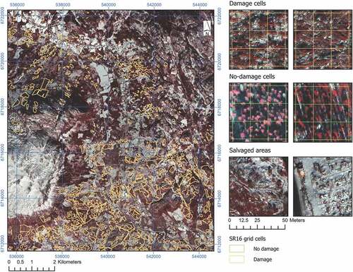
We used a ground reference dataset containing observations of windthrow damage collected during the winter of 2021/2022. The ground reference was a combination of visual interpretation of drone orthomosaics and field observations. Windthrow damage was mapped as vector polygons by the Norwegian forestry insurance company Skogbrand with the goal to identify areas eligible for insurance compensation where the eligibility criteria were overturning and breakage due to strong wind in at least 25% of the pre-storm tree count, excluding patches smaller than 0.2 ha and stands with fewer than 200 stems/ha (Skogbrand Forsikringsselskap Gjensidig 2022a). Since salvage harvesting had been going on for 4 months by the time the satellite stereo images were collected (Section 2.2), we excluded from our analysis 102 salvaged stands (of 853 in total) visually identified in the orthorectified satellite images based on the presence of fresh logging residue and ruts (Figure 1). One-third of the damage polygons were reported as partially damaged, i.e., with less than 50% of the pre-storm tree count felled by wind. Due to the observed inconsistencies in the application of the damage level criterion in the field data, we chose to merge the two damage classes together.

Candidate no-damage areas were identified by combining the areas representing forest estates covered by a wind damage insurance, a forest mask derived from the Norwegian forest resource map SR16 (NIBIO 2022), and the damage polygons, assuming forest areas covered by insurance and not reported as damaged to be free of windthrow damage. No-damage areas smaller than 1 ha were excluded to eliminate artefacts. The resulting 751 damage polygons and the candidate 182 no-damage areas were rasterized on a 16 by 16 m grid aligned with the SR16 map grid as 41,000 damage cells and 168,000 candidate no-damage cells. From the latter, we selected 42,000 (25%) no-damage cells through visual interpretation of the orthorectified VHR satellite images acquired in March 2022 (Section 2.2) by excluding cells containing clear signs of wind damage, cells obviously misclassified as forest, cells that could not be reliably classified due to shadows, and cells representing very sparse woodland and juvenile forest stands. We made sure that the selected no-damage cells contained not only dense forest stands, but also sparser, thinned and higher-elevation forest with narrow crowns, expected to present a challenge for 3D reconstruction of VHR satellite stereo (Goldbergs et al. 2019; Loghin, Otepka-Schremmer, and Pfeifer 2020; Piermattei et al. 2019). The number of no-damage cells was chosen to achieve a prevalence value θ close to 0.5 for the entire dataset. The reference dataset covered 29% of the forest area. Examples of damage and no-damage cells are shown in Figure 1.

We believe that the criteria applied to map windthrow damage in combination with the no-damage cell selection procedure introduced an element of imperfection (false negatives, i.e., wind-damaged patches not recorded as such) into the reference data, which is thus considered imperfect ground reference combining reduced sensitivity (i.e., ability to discriminate against false negatives) with perfect specificity (i.e., ability to discriminate against false positives) (Foody 2010; Yerushalmy 1947).

2.2. VHR satellite imagery

For 3D reconstruction and windthrow damage detection, VHR optical imagery covering the study area was collected by the WV-3 satellite as an along-track stereo pair (one forward- and one backward-looking image) on 6 March 2022. The stereo pair was collected as a combination of one panchromatic (PAN) and eight multispectral (MS) bands and delivered as a View-Ready Standard Stereo (OR2A) product projected onto the WGS-84 ellipsoid with a constant base elevation, calculated as the footprint’s average terrain elevation, and georeferenced using WGS84 UTM Zone 32N (Maxar Technologies 2020c). The OR2A product had a spatial resolution of 0.3 m and 1.2 m for the PAN and MS bands, respectively, and a real dynamic range of 11 bits (stored as 16 bits). Each of the images included rational polynomial coefficients (RPCs) describing the sensor camera model (Grodecki and Dial 2003). Detailed specifications of the stereo pair are given in Table 1.

Table 1. Specifications of the VHR satellite images: WV-3 stereo pair and two GE-1 strips.

Product	WV-3 View-Ready Standard Stereo OR2A		GE-1 System-Ready Basic 1B
Image catalogue ID	104005003EDC4600	104005003EDC4800	10500500FEDD6B00
Collection date and time	6 March 2022, 10 h 39 min 35 s	6 March 2022, 10 h 40 min 19 s	25 November 2021, 10 h 21 min 20 s	25 November 2021, 10 h 21 min 22 s
Cloud cover (%)	0		3	0
Sun azimuth (°)	165.7	165.9	169
Sun elevation (°)	23.2	23.2	8.3	8.2
PAN collected column GSD (m)	0.346	0.324	0.658	0.669
PAN collected row GSD (m)	0.343	0.33	0.816	0.844
PAN product pixel size (m)	0.3	0.3	0.73	0.748
Satellite elevation (°)	68.5	74.6	42	41.1
Satellite azimuth (°)	44.3	153.9	155.3	156.1
Off-nadir view angle (°)	19.5	13.7	42	42.7
Convergence angle (°)	30.1		-

For rigorous accuracy assessment of the classified windthrow damage map of the entire study area, we used an additional VHR product, collected by the GeoEye-1 (GE-1) satellite shortly after the windstorm on 25 November 2021 (Table 1). The collection was a combination of one PAN and four MS (Blue, Green, Red, Near-Infrared) bands, delivered as a System-Ready Basic 1B (L1B) product including RPCs, i.e., ‘raw’ imagery radiometrically and sensor-corrected, but not projected on a plane and thus having a variable pixel resolution (Maxar Technologies 2020b).

2.3. Ground control points, check points and LiDAR digital elevation models (DEMs)

We collected ground control points (GCPs) and independent check points (ICPs) to improve geolocation accuracy and validate the 3D model. WV-3 imagery is reported by the satellite operator Maxar Technologies to possess a horizontal geolocation accuracy of <3.5 m circular error at the 90th percentile (CE90) without the use of GCPs (Maxar Technologies 2020c). This claimed accuracy is in line with the typical geolocation accuracies reported in the literature (e.g., 2.8–2.9 m CE90 for PAN images in Bresnahan, Powers, and Vazquez (2016)). To achieve a root mean square geolocation error of less than 1 pixel (<0.3 m), we collected 33 GCPs and 16 ICPs in an aerial orthomosaic with a spatial resolution of 0.2 m made available by the Norwegian Mapping Authority (Norwegian Mapping Authority and Geovekst 2022). 3D coordinates of the GCPs and ICPs were measured in ETRS89 UTM 32N with orthometric heights using the NN2000 vertical datum.

We used LiDAR-based DSM and DTM from the Norwegian National Digital Elevation Model as the pre-event reference. The LiDAR DSM of the study area had a resolution of 1.08 m and was a combination of three LiDAR surveys flown in 2016–2017 with a point density of 2 to 5 points/m² (Norwegian Mapping Authority 2022); the DTM had a resolution of 1 m.

3. Methods

We implemented the following workflow to detect windthrow damage and conduct rigorous map accuracy assessment:

1. Pre-processing: pan-sharpening of the WV-3 and GE-1 imagery, followed by (1) stereo model generation and refinement of the WV-3 stereo, including accuracy assessment, and (2) orthorectification of the GE-1 imagery.

2. DSM generation by dense image matching of the WV-3 stereo.

3. Assessment of the geolocation and vertical accuracy of the reconstructed DSM on stable ground surfaces.

4. Training and cross-validating a classifier model to predict windthrow damage within the spatial extent of the ground reference dataset.

5. Accuracy assessment of the windthrow damage predictions made for the ground reference dataset using robust performance metrics.

6. Rigorous accuracy assessment using same robust metrics of a windthrow damage map produced by applying the best-performing model to the entire study area.

3.1. Pre-processing of the satellite imagery and bundle adjustment of the stereo pair

We used ENVI ver. 5.6.2 to pre-process the satellite imagery: we pan-sharpened the eight MS bands of the WV-3 stereo pair using the nearest neighbour diffusion-based pan-sharpening algorithm (Sun, Chen, and Messinger 2014) and prepared two band stacks (one per WV-3 image) composed of three pan-sharpened bands each – NIR1, Green, Coastal Blue – for the subsequent 3D reconstruction. The three bands were selected to maximize visual contrast and quality.

We pan-sharpened the GE-1 images by applying two algorithms as implemented in ENVI – the Gram–Schmidt algorithm (Laben and Brower 2000) and the HSV algorithm – to the Red, Green, Blue (RGB) and Near-Infrared, Red, Green (VNIR) band combinations and orthorectified the resulting images using DTM without GCPs (relative orthorectification). The resulting images had a resolution of 0.84 m due to a high off-nadir acquisition angle of 42°.

For bundle adjustment of the stereo pair and 3D reconstruction we used the digital photogrammetry software Agisoft Metashape Pro (ver. 1.8.3). The GCPs and ICPs were first placed in the two WV-3 band stacks to assess geolocation accuracy using the provided RPC model. In the second step, the RPC model was refined to achieve sub-pixel accuracy and another geolocation accuracy assessment was made based on the ICPs alone.

3.2. DSM generation by dense image matching of satellite stereo

Using the two stacks of three pan-sharpened MS bands (Section 3.1), we built two photogrammetric 3D point clouds with two different point densities by using two downscaling factors of 4 and 16 representing the size of the kernel window applied to downsample the original images. Both point clouds had gaps in locations where the dense image matching algorithm (Hirschmüller 2008) failed to match 3D points in object space. As the gaps occurred in different locations depending on the downscaling factor, we merged the two point clouds to fill in the gaps, similarly to the approach taken in Straub et al. (2013), and achieve a point spacing of approximately 0.5 m. We filtered the merged point cloud for low and high noise in ArcGIS Pro ver. 3.0 by applying a minimum and maximum threshold of, respectively, −4 m and 25 m relative to the DTM based on the 90^th percentile of 22.5 m of the dominant tree height in the area of interest (NIBIO 2022) and rasterized it with a spatial resolution of 0.49 m, the highest possible resolution for the merged point cloud.

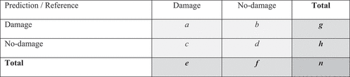
3.3. Accuracy assessment of DSM

We assessed the vertical error ${\mathrm{\Delta }}_h$ on a subsample of 360,000 ground points (86,500 m²) representing snow-free paved road surfaces extracted from the photogrammetric DSM and the reference LiDAR DTM. The effect of road edges and potential misalignment was reduced by buffering to 1.5 m from the centreline. We tested the resulting error distribution for normality using histograms and Q–Q plots and chose to use the four robust statistical metrics suggested by Höhle and Höhle (2009) as less sensitive to non-normal distribution and outliers: the median, the normalized median absolute deviation (NMAD), and the 68.3% and 95% quantiles of the absolute error, i.e., $\left|{\mathrm{\Delta }}_h\right|$. The NMAD was calculated as follows:

(1) $NMAD=1.4826\times {\mathrm{M}}_j\left(\left|{\mathrm{\Delta }}_j-{\mathrm{M}}_{\mathrm{\Delta }}\right|\right),$(1)

where ${\mathrm{\Delta }}_j$ is the individual errors $j=1,\dots ,n$, ${\mathrm{M}}_{\mathrm{\Delta }}$ is the median of the errors, and ${\mathrm{M}}_j$ is the median absolute deviation. The NMAD was chosen as a distribution-free estimator of the scale of distribution, converging with the standard deviation when the distribution is normal, and the 68.3% quantile was chosen to represent the absolute error interval within one standard deviation from the mean, assuming underlying normal distribution (Höhle and Höhle 2009). The uncertainty of the four robust estimators was estimated by finding 95% confidence intervals by bootstrapping with 1000 samples with replacement. All statistical analysis was conducted in the open-source statistical software R (R Core Team 2022).

3.4. Windthrow damage detection

We normalized the photogrammetric and reference DSMs by subtracting the DTM to obtain canopy heights (nDSMs or CHMs) before and after the windstorm, and derived canopy height change between 2017 and 2022 as the difference between the two with same resolution as the WV-3 DSM. We then aggregated canopy height change on the SR16 grid by calculating the height change mean for each SR16 cell. As we expected forest crown closure to affect the performance of 3D canopy reconstruction (Goldbergs et al. 2019; Loghin, Otepka-Schremmer, and Pfeifer 2020; Piermattei et al. 2019), we selected basal area, available from the SR16 map, to represent this effect. In a Nordic boreal forest setting, this variable provides an objective basis for stratifying the forest area into crown closure classes and is commonly available to forest owners.

As the accuracy metric used to optimize the classifier, we chose the Matthews correlation coefficient (MCC, see Equation 4(4) $\widetilde{MCC}=\frac{a\times d-b\times c}{\sqrt{\left(a+b\right)\left(a+c\right)\left(b+d\right)\left(c+d\right)}}$(4) below) (Matthews 1975) – a special case of the phi coefficient, similar to the Pearson correlation coefficient as applied to a matrix of two binary variables (Guilford 1954) – considering its properties of (1) being less sensitive to imbalanced datasets than, e.g., overall accuracy, Cohen’s kappa, and F1 score; and (2) taking into account both true negatives and true positives and thus combining sensitivity and specificity into a single performance score (Chicco and Jurman 2020). MCC has a valid range of [−1, 1], where values above zero indicate performance better than a random classifier.

To produce a binary windthrow map, we trained a thresholding classifier model using canopy height change per SR16 cell as the only input. The threshold value was optimized to maximize the MCC of the resulting two-class confusion matrix (Baldi et al. 2000). For threshold optimization we used the R package cutpointr (Thiele and Hirschfeld 2021). The model was trained and validated by K-fold cross-validation with K = 10. Threshold values were averaged over the ten folds and applied as a binary classification rule to the entire reference dataset.

A stratified version of the model was additionally trained, where we subdivided the reference dataset into three strata according to the basal area (BA) value: low BA (<15 m²/ha, n = 17,873, θ = 0.33), moderate BA (15–30 m²/ha, n = 39,798, θ = 0.49), and high BA (≥30 m²/ha, n = 26,199, θ = 0.6). The threshold was optimized for each of the strata separately, and the stratified model’s performance was compared to that achieved for the given stratum with the non-stratified threshold.

3.5. Classification accuracy assessment

Two-by-two confusion matrices (Figure 2) were built for the classifier and its stratified version, and classification accuracy was reported using three accuracy measures: sensitivity $S_1$, specificity $S_2$, and the Matthews correlation coefficient MCC (Chicco and Jurman 2020). These measures were chosen considering their predictable behaviour in response to the effects of error in the ground reference data at different prevalence levels θ of the damage class (Fielding and Bell 1997; Foody 2010). Additionally, we calculated the value of the area under the receiver operating characteristic (ROC) curve (AUC) for each of the models. The ground reference data was considered to be imperfect (Section 2.1): we arbitrarily set its sensitivity $S_1^{\mathrm{R}}$ to 0.9 and specificity $S_2^{\mathrm{R}}$ to 1. The assumed imperfection is based on the consideration that windthrown patches of forest either under 0.2 ha (Section 2.1) or poorly visible in the VHR imagery were likely to be registered as no-damage areas (error of omission, i.e., less than perfect sensitivity $S_1^{\mathrm{R}}$). The value of $S_1^{\mathrm{R}}$ was chosen arbitrarily to illustrate the direction and magnitude of the effect of imperfect ground reference on sensitivity and specificity at the apparent prevalence level θ of 0.5. Errors in the ground reference and in the classifier predictions were assumed to be conditionally independent (Foody 2010).

Figure 2. Two-by-two (binary) confusion matrix where each observation is placed in one of the four cells based on the relationship between the predicted and reference value.

In addition to the perceived values of $\widetilde{MCC}$, sensitivity $\widetilde{S_1}$ and specificity $\widetilde{S_2}$, we calculated the true values of sensitivity and specificity adjusted for the assumed error ($S_1$, $S_2$,) (Chicco and Jurman 2020; Foody 2011; Staquet et al. 1981) as follows:

(2) $\widetilde{S_1}=\frac{a}{e}$(2)

(3) $\widetilde{S_2}=\frac{d}{f}$(3)

(4) $\widetilde{MCC}=\frac{a\times d-b\times c}{\sqrt{\left(a+b\right)\left(a+c\right)\left(b+d\right)\left(c+d\right)}}$(4)

(5) $S_1=\frac{g{S}_2^{\mathrm{R}}-b}{n\left(S_2^{\mathrm{R}}-1\right)+e}$(5)

(6) $S_2=\frac{h{S}_1^{\mathrm{R}}-c}{n{S}_1^{\mathrm{R}}-e}$(6)

where $a,b,c,d,e,f,g,h,n$ refer to the cell values and totals as shown in Figure 2.

3.6. Map accuracy assessment

We produced a classified windthrow map of the study area by applying the trained classifier to a forest mask derived from the SR16 map. For rigorous map accuracy assessment as described in Olofsson et al. (2014), we chose visual interpretation of an additional set of random points using a combination of the GE-1 and WV-3 imagery (Section 2.2). We randomly selected 400 cells from within the forest mask and visually classified these as either damage or no-damage. If a cell was found to be a mixed cell or a non-forest cell or was hard to interpret because of image quality, it was discarded. After filtering, 283 valid cells (160 damage and 123 no-damage) were used to produce two-by-two confusion matrices, and map accuracy assessment was carried out as described in Section 3.5 using perceived sensitivity $\widetilde{S_1^{\mathrm{M}}}$, specificity $\widetilde{S_2^{\mathrm{M}}}$, and $\widetilde{MC{C}^{\mathrm{M}}}$. We did not correct the accuracy measures for potential error in the ground reference because the magnitude of such error would be difficult to estimate. The map accuracy assessment dataset had a prevalence θ of 0.57.

4. Results

4.1. Geolocation accuracy of the 3D model

The 3D model based on the RPCs alone had a geolocation error (reported as RMSE) of 0.52 m horizontally and 0.14 m vertically when measured using the 33 GCPs and of 0.88 m and 1.12 m, respectively, when measured using the 16 ICPs. After optimization using GCPs, the error was reduced to 0.15 m horizontally and 0.03 m vertically on the GCPs, 0.44 m and 0.46 m on the ICPs (Table 2). Geolocation accuracy was thus <1 image pixel if measured on GCPs and slightly above 1 pixel on ICPs. This is in line with the geolocation accuracy values reported for WorldView-2 by Aguilar, Saldaña, and Aguilar (2014), Poli et al. (2015), Hobi and Ginzler (2012) and for WorldView-3 by St-Onge and Grandin (2019).

Table 2. Geolocation accuracy of the reconstructed 3D model before and after GCP optimization, RMSE in m.

Error measurement locations	Error before RPC optimization (m)		Error after RPC optimization (m)
	Horizontal	Vertical	Horizontal	Vertical
GCPs	0.52	0.14	0.15	0.03
ICPs	0.88	1.12	0.44	0.46

4.2. DSM accuracy

The photogrammetric DSM was found to have a vertical accuracy on the same order of magnitude as the spatial resolution of the WV-3 stereo pair and the geolocation accuracy of the 3D model.

We found that the median height error (systematic shift) of the photogrammetric DSM when compared to the reference DSM on paved road surfaces was −44 cm with multiple strongly positive outliers caused by parts of tree crowns located directly above the road surfaces (Table 3). The mean error (−40 cm) deviated from the median (−44 cm), consistent with a moderate positive skewness of 7.3. The distribution-independent estimator NMAD (49 cm) was found to be narrower than the standard deviation (56 cm), indicating a peaked distribution.

Table 3. Accuracy measures, including robust, distribution-independent ones, for the photogrammetric DSM.

Accuracy measures assuming normal distribution	Notation	Value
Mean error (cm)	$\hat{\mu }$	−40.75
Standard deviation (cm)	$\hat{\sigma }$	55.86
Skewness		7.3
Kurtosis		132.23
Robust accuracy measures	Error type	Value	95% confidence interval (cm)
Median (cm)	Δh	−43.8	[−43.94, −43.67]
NMAD (cm)	Δh	49.29	[49.09, 49.48]
68.3% quantile (cm)	|Δh|	60.96	[60.82, 61.11]
95% quantile (cm)	|Δh|	106	[105.8, 106.6]

Error ${\mathrm{\Delta }}_h$ distribution of the photogrammetric DSM presented as a histogram and a normal Q–Q plot in Figure 3 is non-normal with a strong peak and a long right-hand tail indicating a greater share of severe positive outliers than negative ones. This finding is supported by the NMAD (49 cm) being narrower than the 68.3% quantile (61 cm). Therefore, we consider the four robust metrics – median error, NMAD, 68.3% and 95% quantiles – to be more appropriate accuracy measures.

Figure 3. Histograms (a) and normal Q–Q plot (b) of the photogrammetric DSM error distribution. For readability, the histogram (bin width 10 cm) is also presented for three separate intervals with different scaling of the vertical axis: −4 m to −2 m, −2 m to +1 m, and +1 m to +16 m.

4.3. Windthrow damage classification accuracy

The classifier model demonstrated a reasonable level of accuracy, with a preference for specificity $S_2$ vs. sensitivity $S_1$. As follows from Equations 5(5) $S_1=\frac{g{S}_2^{\mathrm{R}}-b}{n\left(S_2^{\mathrm{R}}-1\right)+e}$(5) and 6(6) $S_2=\frac{h{S}_1^{\mathrm{R}}-c}{n{S}_1^{\mathrm{R}}-e}$(6) , the perceived sensitivity $\widetilde{S_1}$ was unaffected by the less than perfect sensitivity of the ground reference; at the same time, perceived specificity $\widetilde{S_2}$ was substantially underestimated compared to the true value of $S_2$ (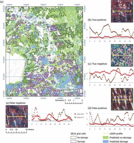0.785 vs. 0.841). Figure 4 presents a classified windthrow map, including examples of correctly classified and misclassified cells.

Figure 4. Classified windthrow map of the study area on the SR16 grid using the non-stratified thresholding classifier (a). Examples of correctly classified and misclassified cells, including respective nDSM profiles extracted from the reference and photogrammetric nDSMs (b) – (e). Axes in (b) – (e) are in m, blue dotted guidelines in indicate ground surface where the photogrammetric nDSM has negative elevations. Coordinates are given in ETRS89 UTM 32N. (Satellite imagery © 2023 Maxar Technologies).

Table 5(a) reports the classification accuracy measures for the thresholding classifier model stratified by BA (Section 3.5) with the threshold value optimized per stratum. For comparison, classification accuracy is also presented in Table 5(b) for the original non-stratified thresholding model with a breakdown into the BA strata. Stratifying the classification threshold failed to materially improve the classification accuracy as measured by $\widetilde{MCC}$ and at the same time, introduced a strong bias towards sensitivity S₁, especially in the low and moderate BA strata. The stratified threshold value differed greatly between the strata – from close to zero (−0.65 m) in the low BA stratum to a strongly negative value of −3.62 m (close to the non-stratified value of −3.56 m) in the high BA stratum.

Table 4. Accuracy measures (perceived values, estimates of real values assuming $S_1^{\mathrm{R}}=0.9$, $S_2^{\mathrm{R}}=1$ are given in brackets, where applicable) of the thresholding classifier using canopy height change as the input.

Model	Threshold value (m)	$\widetilde{MCC}$	$\widetilde{S_1}$ ($S_1$)	$\widetilde{S_2}$ ($S_2$)	AUC
Thresholding classifier	−3.56	0.465	0.677 (0.677)	0.785 (0.841)	0.806

Table 5. Stratum-level accuracy measures (perceived values, estimates of real values assuming $S_1^{\mathrm{R}}=0.9$ are given in brackets, where applicable) of the stratified canopy height change-based classifier (a), compared to a breakdown of the original non-stratified model by BA class (b). AUC values are unaffected by stratification and thus identical in (a) and (b).

Model	Threshold value (m)	$\widetilde{MCC}$	$\widetilde{S_1}$ ($S_1$)	$\widetilde{S_2}$ ($S_2$)	AUC
(a) Stratified classifier
Low BA (n = 17,873, θ = 0.33)	−0.65	0.112	0.920 (0.920)	0.162 (0.166)	0.597
Moderate BA (n = 39,798, θ = 0.49)	−2.73	0.392	0.836 (0.836)	0.540 (0.585)	0.764
High BA (n = 26,199, θ = 0.6)	−3.62	0.641	0.895 (0.895)	0.732 (0.858)	0.867
(b) Non-stratified classifier, breakdown by BA class
Low BA	−3.56	0.095	0.043 (0.043)	0.987 (0.989)	0.597
Moderate BA		0.384	0.690 (0.690)	0.694 (0.740)	0.764
High BA		0.640	0.896 (0.896)	0.729 (0.856)	0.867

We found that the imperfect sensitivity $S_1^{\mathrm{R}}$ of the ground reference resulted in systematic underestimation of the perceived specificity $\widetilde{S_2}$ in all strata when compared to the true specificity $S_2$. The underestimation effect was most pronounced in the moderate and high BA classes, where $S_2$ (0.74 and 0.856) was, respectively, 0.046 and 0.127 higher than $\widetilde{S_2}$ (Table 5(b)).

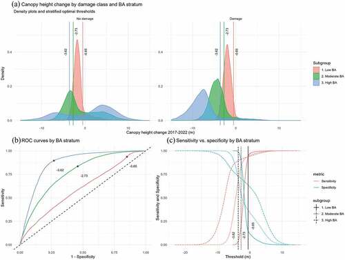
Figure 5(a,b) shows density plots of the damage and no-damage classes grouped by BA stratum and the respective ROC curves of the stratified thresholding classifier. The low BA stratum has a ROC curve close to that of a random classifier (AUC 0.597, see Table 5), explained by the almost identical density distributions of the damage and no-damage classes distinguished solely by the slim right-hand tail of positive canopy height change values in the no-damage class. The shape of the ROC curves (and accordingly, the AUC values of 0.764 and 0.867 in the higher BA strata, see Table 5) improved with increasing BA values, supported by the better separation of the damage and no-damage classes in the moderate and high BA strata. The no-damage class distributions had peaks in the negative height change region (Figure 5(a)), more prominent in the lower BA strata, – these resulted from a combination of the error of omission $\left(S_1^R=0.9\right)$ in the ground reference (Section 3.5) and dense image matching errors (Section 3.2). Figure 5(a) indicates that, based on the relative shape of the density plots for the no-damage class, the high BA stratum was less prone to imperfect $S_1^R$ and reduced $S_2$ compared to the moderate BA stratum.

Figure 5. Density plots of the canopy height change value in the no-damage and damage classes stratified by BA (a); ROC curves for the three BA strata (b); and sensitivity vs. specificity plot of the thresholding classifier, stratified by BA (c). Vertical lines in (a) and (c) and points on the curves in (b) show optimal threshold values in m by BA stratum.

4.4. Classified map accuracy

Table 6 shows map-level and stratum-level perceived accuracy measures resulting from rigorous map accuracy assessment of the non-stratified thresholding classifier. On both levels, there was a slight improvement over the respective values reported in Tables 4 and 5(b) except for the low BA stratum.

Table 6. Map-level (a) and stratum-level (b) rigorous map accuracy assessment (perceived values) on an extended set of imagery (n = 283) of the classified windthrow damage map (Figure 4).

Accuracy assessment	$\widetilde{S_1^{\mathrm{M}}}$	$\widetilde{S_2^{\mathrm{M}}}$	$\widetilde{MC{C}^{\mathrm{M}}}$
(a) Map-level accuracy	0.775	0.732	0.505
(b) Stratum-level accuracy by BA class
Low BA	0.0	0.952	−0.152
Moderate BA	0.785	0.672	0.460
High BA	0.961	0.711	0.718

On the map level, rigorous map accuracy assessment showed a slightly higher $\widetilde{MC{C}^{\mathrm{M}}}$ of 0.505 (Table 6(a)), compared to 0.465 in Table 4. We found the classified windthrow damage map to have a higher sensitivity $\widetilde{S_1^{\mathrm{M}}}$ (0.775) than specificity $\widetilde{S_2^{\mathrm{M}}}$ (0.732), in contrast to our earlier finding of higher specificity $\widetilde{S_2}$ (Table 4).

On the stratum level, map accuracy assessment revealed a negative $\widetilde{MC{C}^{\mathrm{M}}}$ of −0.152 in the low BA stratum (Table 6(b)), caused by the model’s zero sensitivity $\widetilde{S_1^{\mathrm{M}}}$. In the moderate and high BA strata, we found $\widetilde{MC{C}^{\mathrm{M}}}$ to be higher than the respective $\widetilde{MCC}$ values in Table 5(b) − 0.46 vs. 0.384 (moderate BA) and 0.718 vs. 0.64 (high BA). Similarly to the map level, the classified windthrow damage map was consistently more sensitive than specific in denser forest stands, i.e., better able to discriminate against false negatives than false positives.

5. Discussion

This study demonstrated that windthrow damage can be detected as a decrease in forest canopy height from a pre-storm to a post-storm DSM obtained by 3D reconstruction of WV-3 stereo imagery. The utility of the method is limited to moderate-to-high density productive boreal conifer forest stands, where accurate windthrow maps could be produced even under suboptimal imagery collection conditions, such as sun elevation lower than 25° and presence of snow.

5.1. Mapping windthrow with VHR stereo optical satellite imagery

Major windstorms caused by extratropical cyclones forming in the North Atlantic tend to hit the Nordic countries during the late autumn and winter months (Feser et al. 2015; Gregow, Laaksonen, and Alper 2017), posing operational challenges for the collection of optical satellite imagery at higher latitudes due to a combination of persistent cloud cover, low sun elevation, poor lighting conditions, and snow cover. Specifications of the collected GE-1 imagery in Table 1 offer an illustration of such challenges: the GE-1 imagery was acquired during a short cloud-free window within 1 week after the windstorm and had both a high off-nadir angle of 42° and a low sun elevation of slightly above 8°, i.e., conditions considered unfavourable for stereophotogrammetric reconstruction (Piermattei et al. 2018; Qin 2019). Once the location of windthrow damage is known, the spatial extent of the area to be covered by 3D reconstruction-based windthrow mapping does not appear to be a practical limitation as a single stereo collection scenario by, e.g., WV-3 can have a footprint of up to 2900 km² (Maxar Technologies 2020a) and can be combined with collections by other VHR satellites in the same or different constellation.

During the winter months, 3D reconstruction of optical VHR imagery can be combined with bitemporal change detection or time-series analysis using lower-resolution optical satellite imagery collected continuously (e.g., by Sentinel-2 or the PlanetScope constellation) and synthetic aperture radar (SAR) imagery products collected by active spaceborne sensors irrespective of cloud cover and lighting conditions (e.g., TerraSAR-X/TanDEM-X and the Capella Space and ICEYE constellations). Such alternative methods using lower-resolution optical satellite imagery are reported to have classification accuracies close to those achieved in this study (Chehata et al. 2014; Dalponte et al. 2020), but may involve long waiting time until imagery of satisfactory quality is collected over an entire region of interest (Vaglio Laurin et al. 2020). A combination of mutually complementary methods offering different trade-offs regarding the levels of detail, accuracy and acquisition cadence appears thus to be the optimal solution for large-scale windthrow mapping (Schwarz et al. 2003).

In this study, we chose forest canopy height change between two timepoints as the main input variable to the windthrow classification models, rather than the spectral information stored in WV-3’s eight MS bands (Maxar Technologies 2020a) or the spectral indices using those, such as NDVI (Tucker 1979). The rationale behind this choice was to make the proposed windthrow detection workflow insensitive to such effects on the forest canopy spectral properties as species composition and phenological variation, presence of snow, tree crown shadows and lighting conditions, and to make the classification model as generalizable as possible.

Earlier work indicates that forest canopy height can be measured by digital stereophotogrammetry with an error that is one order of magnitude smaller than mean canopy height in a mature boreal conifer forest (Goldbergs 2021; Goldbergs et al. 2019; Loghin, Otepka-Schremmer, and Pfeifer 2020; Montesano et al. 2017; Persson and Perko 2016; Piermattei et al. 2018, 2019; St-Onge and Grandin 2019; St‐Onge, Hu, and Vega 2008), implying the possibility of reliably detecting both uprooting and stem breakage, both causing a major reduction in canopy height exceeding the measurement error.

5.2. Photogrammetric DSM accuracy

Our findings on geolocation accuracy (Section 4.1) are in line with the earlier reports on the high accuracy of photogrammetric DEMs derived from VHR stereo acquisitions, in particular by the WV-2/3 satellites (Aguilar et al. 2019; Aguilar, Saldaña, and Aguilar 2013; Hobi and Ginzler 2012; Poli et al. 2015; Wang et al. 2019). On uniform surfaces and in relatively flat terrain, horizontal and vertical accuracies comparable to image pixel size, i.e., 0.3 m for WV-3, can be achieved by refining the stereo model using as few as 10–15 GCPs (Nowak Da Costa 2010; Perko et al. 2014; Persson 2016; Perko, Raggam, and Roth 2019; Vajsova et al. 2015), compared to the 33 GCPs we chose to collect in this study to account for the complex topography in the study area. The reconstructed 3D model was consistently less accurate when measured on ICPs, compared to GCPs (Table 2); this is an expected finding as RPC optimization fits the 3D model to the GCPs. Still, RPC optimization at least halved both horizontal and vertical error as measured on ICPs (Table 2), resulting in a vertical accuracy close to 0.33 m as reported for WV-2 in Hobi and Ginzler (2012).

Our DSM accuracy assessment results were consistent in terms of error magnitude with the findings on the vertical accuracy of the 3D model as measured on ICPs, and additionally revealed that (1) the photogrammetric DSM underestimated height by a median of 0.44 m (Table 3, Figure 3) and (2) despite some severe positive outliers (Figure 3), the 95% quantile of the absolute vertical error was only slightly greater than 1 m (Table 3). A possible explanation for the observed systematic underestimation of road surface elevations is that very few of the GCPs were located on paved road surfaces, while the DSM subset used for accuracy assessment was a collection of linear features representing a small fraction of the study area. The median elevation error (−0.44 m) in this study was larger than −0.26 m as measured on man-made surface in a photogrammetric DSM derived from a WV-2 stereo pair in Hobi and Ginzler (2012), however the NMAD was lower in this study (0.49 m) compared to 0.86 m in the cited paper, indicating a more peaked error distribution.

We were prevented from comparing the photogrammetric CHM over intact forest with a more accurate reference dataset, such as airborne LiDAR, due to the unavailability of reference data for the study area more recent than 2017–2019. This is a limitation of this study that could potentially be overcome by using, e.g., ICESat-2 spaceborne LiDAR data, similarly to Montesano et al. (2017), subject to the availability of ICESat-2 tracks in intact forest areas. Reported CHM accuracies expressed as RMSE range from 1.4 m to 2.04 m for WV-2 (Persson and Perko 2016; Ullah et al. 2020; Yu et al. 2015). Tian et al. (2017) reported a NMAD of 3.66 m in dense forest and 5.25 m in less dense forest for a WV-2 photogrammetric DSM. When comparing photogrammetric single-tree height measurements using a WV-3 stereopair to the tree heights as measured in field, St-Onge and Grandin (2019) found an RMSE of 1.27 m. We expect thus that the photogrammetric CHM accuracy in this study is no worse than the RMSE values reported for WV-2/3, with potential outliers in sparser forest stands.

Considering the CHM accuracies above, the proposed method appears to be sufficiently accurate, despite the time gap of 5 years between the photogrammetric DSM and the pre-storm LiDAR DEM. Tree uprooting results in a canopy height reduction of up to 15–30 m, which by an order of magnitude exceeds both the typical height increment in mature boreal forest, ranging between 1.5 and 3 m or more over a five-year period (Kvaalen, Solberg, and May 2015), and a conservative canopy height RMSE estimate of 3 m. Same logic applies to stem breakage as tree stems have insufficient cross-section to be photogrammetrically reconstructed as a continuous surface (Goldbergs 2021).

5.3. Windthrow detection accuracy

To the best of our knowledge, few studies exist where 3D reconstruction of VHR satellite stereo imagery is employed to detect and map forest windthrow. One of these is Tian et al. (2017) where a post-storm WV-2 photogrammetric DSM was compared to a pre-storm LiDAR DSM, however the WV-2 imagery was collected 5 years after the windstorm, making their findings less relevant to the operational post-event mapping context.

We consider more realistic the presented scenario where satellite imagery is collected shortly after a windstorm when few alternative VHR sources are available. In that context, the ground reference data can both be expected to be scarce and incomplete and contain error, such as horizontal shift due to improper georeferencing, misclassified transitional cases (Foody 2010), bias introduced by applying arbitrary classification criteria or by generalization techniques used, e.g., morphological operators (Tian et al. 2017). However, the magnitude of error is hard to estimate and can range from 15% (Foody 2010) to 60% (Thompson et al. 2007). It is therefore important to characterize the often-predictable effect on the classification accuracy estimates of imperfections in the ground reference considering that the change class prevalence may vary (Foody 2010, 2011). Finally, we consider it relevant to not only check whether forest stand attributes, such as BA, can improve windthrow detection performance, but also examine how sensitive the classifier is to forest conditions other than fully stocked productive stands.

Loghin, Otepka-Schremmer, and Pfeifer (2020) reported that WV-3 photogrammetric CHMs cannot reliably estimate tree height in conifers with narrow crowns <2.5 m (<8 image pixels) in diameter, resulting in a reconstructed tree height of <50% of the actual height. However, in conifers with crowns >5 m (>16 pixels), >90% of the actual tree height was reconstructed. This is consistent with the findings that dense image matching of VHR stereo is challenging in open-canopy forests (Goldbergs et al. 2019) when the sun elevation angle is above 25° (Montesano et al. 2017). In our study, the clear effect of BA as a proxy for crown closure on the classification performance is evident from Table 6 – with a decreasing BA in boreal thinned or high-elevation forest stands, crown diameter tends also to decrease, and the forest canopy becomes discontinuous, causing a drop in the tree crown detection rate and a false positive classification outcome. While crown closure is not a forest stand metric commonly available as part of national forest inventories, BA is widely available and tends to correlate with the forest stand’s development stage and thus crown closure, becoming a useful sensitivity metric in 3D reconstruction of a forest canopy in a setting similar to the one described in this study.

Figure 5(a) demonstrates that in the low BA stratum, the damage and no-damage classes have an almost identical canopy height change distribution – apart from a more pronounced right-hand tail in the no-damage class, both classes have their peaks at −2 m. This explains the very different $\widetilde{S_1}$ and $\widetilde{S_2}$ values in the stratified and non-stratified models: the former was optimized for the low BA stratum by choosing a sensitive threshold of -0.65 m, while in the latter one, the low BA stratum is a minority class and the single threshold is optimized for the majority class, i.e., the moderate and high BA strata, giving a much less sensitive threshold of -3.56 m and a higher $\widetilde{S_2}$ at the expense of a major increase in false negatives.

The most plausible explanation for the nearly identical canopy height change distribution of the damage and no-damage classes in the low BA stratum is a combined effect of the low tree crown detection rate and the imperfect ground reference (reduced sensitivity $S_1^{\mathrm{R}}$).

The assumed imperfections in the ground reference also affect the moderate and high BA strata, but to a much lower extent Figure 5(a): the no-damage class in the moderate BA stratum exhibits a stronger positive tail and a less pronounced peak in the negative region, and the high BA stratum has a well-expressed bimodal distribution dominated by positive values. Shapes of the ROC curves in Figure 5(b) illustrate the improvement in the model’s ability to discriminate with increasing BA.

Another potential misclassification factor, acting irrespective of the BA, are the smooth edges (e.g., between forest and non-forest) characteristic of photogrammetric satellite DSMs and caused by a combination of a lower GSD as compared to a LiDAR DSM and pixels representing tree crown sides that failed to be reliably matched in the 3D reconstruction process. This edge effect might increase the fraction of false negatives by extending the forest canopy beyond its actual boundary, especially in case of partial wind damage where intact trees are interspersed with uprooted ones. We believe that in this study, the edge effect had only a minor impact on the windthrow classification accuracy because of the severity of the wind damage; however, it is to be taken into consideration when applying the proposed workflow to less severe wind damage events.

This study examines a case of severe windthrow concentrated in a small study area with a prevalence θ of 0.5 across the three BA strata (from 0.33 in the low BA to 0.6 in the high BA stratum), which may not apply to windstorms less severe than the 19 November 2021 event and resulting in a diffuse spatial pattern with a lower prevalence.

Rigorous map accuracy assessment (Table 6) was generally consistent with the findings on model accuracy, confirming that a single threshold makes the model insensitive to windthrow in sparse forest. The choice of whether to stratify the threshold should be governed by the classified map user’s preferences and cost functions associated with false negatives vs. false positives and the expected 3D reconstruction performance (Piermattei et al. 2019).

We chose a grid-based approach for this study since the auxiliary data, such as the SR16-derived forest mask and forest attributes, followed that format. Aggregating canopy height change over a 16 × 16 m cell simplifies the windthrow detection workflow, simultaneously making the classifier more prone to false positives. Alternative workflows would involve applying morphological filters to a canopy height change raster (Honkavaara, Litkey, and Nurminen 2013) or undertaking pre- and post-damage tree crown segmentation to detect canopy height change on a single-tree level (Gomes and Maillard 2016; Skurikhin, McDowell, and Middleton 2016; Tong et al. 2021; Wagner et al. 2018).

6. Conclusion

VHR satellite stereo imagery is a viable source of forest canopy height information sufficiently accurate to map forest disturbances such as windthrow that can be combined with bitemporal change detection and time-series analysis methods for region-scale mapping of wind damage. Using the proposed photogrammetric DSM reconstruction workflow and a simple thresholding model requiring no inputs other than canopy height change, accurate windthrow maps can be produced in moderate-to-high density productive forest stands. One limitation of the proposed workflow is that it is less reliable in sparse and high-elevation forest stands. Another limitation is the dependence on the availability of a relatively recent pre-event DSM and of pre-event data on BA or other measure of crown closure.

Acknowledgements

The authors are grateful to the forestry insurance company Skogbrand Forsikringsselskap Gjensidig for sharing the ground reference data on windthrow damage.

Disclosure statement

No potential conflict of interest was reported by the author(s).

Data availability statement

The data that support the findings of this study are available from the corresponding author, PZ, upon reasonable request. Restrictions may apply to the availability of the source data, which were used under licence for this study and are available from the corresponding author with the permission of Maxar Technologies, Inc.

Additional information

Funding

This work was supported by the Research Council of Norway under Grant 301745.

References

- Aguilar, M. A., A. Nemmaoui, F. J. Aguilar, and R. Qin. 2019. “Quality Assessment of Digital Surface Models Extracted from WorldView-2 and WorldView-3 Stereo Pairs Over Different Land Covers.” GIScience & Remote Sensing 56 (1): 109–129. https://doi.org/10.1080/15481603.2018.1494408.
- Aguilar, M. A., M. D. M. Saldaña, and F. J. Aguilar. 2013. “Assessing Geometric Accuracy of the Orthorectification Process from GeoEye-1 and WorldView-2 Panchromatic Images.” International Journal of Applied Earth Observation and Geoinformation 21:427–435. https://doi.org/10.1016/j.jag.2012.06.004.
- Aguilar, M. A., M. D. M. Saldaña, and F. J. Aguilar. 2014. “Generation and Quality Assessment of Stereo-Extracted DSM from GeoEye-1 and WorldView-2 Imagery.” IEEE Transactions on Geoscience and Remote Sensing 52 (2): 1259–1271. https://doi.org/10.1109/TGRS.2013.2249521.
- Baldi, P., S. Brunak, Y. Chauvin, C. A. F. Andersen, and H. Nielsen. 2000. “Assessing the Accuracy of Prediction Algorithms for Classification: An Overview.” Bioinformatics 16 (5): 412–424. https://doi.org/10.1093/bioinformatics/16.5.412.
- Blennow, K., and Erik, P. 2013. ”Societal Impacts of Storm Damage.” in Living with Storm Damage to Forests. What Science Can Tell Us 3, edited by Barry Gardiner, Andreas Schuck, Mart-Jan Schelhaas, Christophe Orazio, Kristina Blennow and Bruce Nicoll, 70–79. Joensuu, Finland: European Forest Institute. https://efi.int/sites/default/files/files/publication-bank/2018/efi_wsctu3_2013.pdf.
- Brandt, M., C. J. Tucker, A. Kariryaa, K. Rasmussen, C. Abel, J. Small, J. Chave, et al. 2020. “An Unexpectedly Large Count of Trees in the West African Sahara and Sahel.” Nature 587 (7832): 78–82. https://doi.org/10.1038/s41586-020-2824-5.
- Bresnahan, P., R. Powers, and L. H. Vazquez. 2016. “WorldView-3 Geolocation Accuracy and Band Co-Registration Analysis.” Paper presented at the 15th JACIE (Joint Agency Commercial Imagery Evaluation) Workshop, co-located with ASPRS Imaging and Geospatial Technology Forum, April 2016, Fort Worth, Texas.
- Chehata, N., C. Orny, S. Boukir, D. Guyon, and J. P. Wigneron. 2014. “Object-Based Change Detection in Wind Storm-Damaged Forest Using High-Resolution Multispectral Images.” International Journal of Remote Sensing 35 (13): 4758–4777. https://doi.org/10.1080/01431161.2014.930199.
- Chicco, D., and G. Jurman. 2020. “The Advantages of the Matthews Correlation Coefficient (MCC) Over F1 Score and Accuracy in Binary Classification Evaluation.” BMC Genomics 21 (1): 6. https://doi.org/10.1186/s12864-019-6413-7.
- Dalponte, M., S. Marzini, Y. Tatiana Solano-Correa, G. Tonon, L. Vescovo, and D. Gianelle. 2020. “Mapping Forest Windthrows Using High Spatial Resolution Multispectral Satellite Images.” International Journal of Applied Earth Observation and Geoinformation 93:102206. https://doi.org/10.1016/j.jag.2020.102206.
- Dowman, I., K. Jacobsen, G. Konecny, and R. Sandau. 2022. High Resolution Optical Satellite Imagery. 2nd ed. Caithness, Scotland: Whittles Publishing.
- Fassnacht, F. E., D. Mangold, J. Schäfer, M. Immitzer, T. Kattenborn, B. Koch, and H. Latifi. 2017. “Estimating Stand Density, Biomass and Tree Species from Very High Resolution Stereo-Imagery – Towards an All-In-One Sensor for Forestry Applications?” Forestry: An International Journal of Forest Research 90 (5): 613–631. https://doi.org/10.1093/forestry/cpx014.
- Feser, F., M. Barcikowska, O. Krueger, F. Schenk, R. Weisse, and L. Xia. 2015. “Storminess Over the North Atlantic and Northwestern Europe—A Review.” Quarterly Journal of the Royal Meteorological Society 141 (687): 350–382. https://doi.org/10.1002/qj.2364.
- Fielding, A. H., and J. F. Bell. 1997. “A Review of Methods for the Assessment of Prediction Errors in Conservation Presence/Absence Models.” Environmental Conservation 24 (1): 38–49. https://doi.org/10.1017/S0376892997000088.
- Foody, G. M. 2010. “Assessing the Accuracy of Land Cover Change with Imperfect Ground Reference Data.” Remote Sensing of Environment 114 (10): 2271–2285. https://doi.org/10.1016/j.rse.2010.05.003.
- Foody, G. M. 2011. “Impacts of Imperfect Reference Data on the Apparent Accuracy of Species Presence–Absence Models and Their Predictions.” Global Ecology and Biogeography 20 (3): 498–508. https://doi.org/10.1111/j.1466-8238.2010.00605.x.
- Francini, S., R. E. McRoberts, F. Giannetti, M. Mencucci, M. Marchetti, G. S. Mugnozza, and G. Chirici. 2020. “Near-Real Time Forest Change Detection Using PlanetScope Imagery.” European Journal of Remote Sensing 53 (1): 233–244. https://doi.org/10.1080/22797254.2020.1806734.
- Goldbergs, G. 2021. “Impact of Base-To-Height Ratio on Canopy Height Estimation Accuracy of Hemiboreal Forest Tree Species by Using Satellite and Airborne Stereo Imagery.” Remote Sensing 13 (15): 2941. https://doi.org/10.3390/rs13152941.
- Goldbergs, G., S. W. Maier, S. R. Levick, and A. Edwards. 2019. “Limitations of High Resolution Satellite Stereo Imagery for Estimating Canopy Height in Australian Tropical Savannas.” International Journal of Applied Earth Observation and Geoinformation 75:83–95. https://doi.org/10.1016/j.jag.2018.10.021.
- Gomes, M. F., and P. Maillard. 2016. “Detection of Tree Crowns in Very High Spatial Resolution Images.” In Environmental Applications of Remote Sensing, edited by M. Maged, 41–73. Rijeka, Croatia: IntechOpen. https://doi.org/10.5772/62122.
- Gregow, H., A. Laaksonen, and M. E. Alper. 2017. “Increasing Large Scale Windstorm Damage in Western, Central and Northern European Forests, 1951–2010.” Scientific Reports 7 (1): 46397. https://doi.org/10.1038/srep46397.
- Gregow, H., M. Rantanen, T. K. Laurila, and A. Mäkelä. 2020. Review on winds, extratropical cyclones and their impacts in Northern Europe and Finland. Report 2020:3. Helsinki, Finland: Finnish Meteorological Institute.
- Grodecki, J., and G. Dial. 2003. “Block Adjustment of High-Resolution Satellite Images Described by Rational Polynomials.” Photogrammetric Engineering & Remote Sensing 69 (1): 59–68. https://doi.org/10.14358/PERS.69.1.59.
- Guilford, J. P. 1954. Psychometric Methods. 2nd ed. New York: McGraw-Hill.
- Hanewinkel, M., and Jean, L. P. 2013. ”The Economic Impact of Storms.” In Living with Storm Damage to Forests. What Science Can Tell Us 3, edited by Barry Gardiner, Andreas Schuck, Mart-Jan Schelhaas, Christophe Orazio, Kristina Blennow and Bruce Nicoll, 55–64. Joensuu, Finland: European Forest Institute. https://efi.int/sites/default/files/files/publication-bank/2018/efi_wsctu3_2013.pdf.
- Hirschmüller, H. 2008. “Stereo Processing by Semiglobal Matching and Mutual Information.” IEEE Transactions on Pattern Analysis and Machine Intelligence 30 (2): 328–341. https://doi.org/10.1109/TPAMI.2007.1166.
- Hobi, M. L., and C. Ginzler. 2012. “Accuracy Assessment of Digital Surface Models Based on WorldView-2 and ADS80 Stereo Remote Sensing Data.” Sensors 12 (5): 6347–6368. https://doi.org/10.3390/s120506347.
- Höhle, J., and M. Höhle. 2009. “Accuracy Assessment of Digital Elevation Models by Means of Robust Statistical Methods.” ISPRS Journal of Photogrammetry and Remote Sensing 64 (4): 398–406. https://doi.org/10.1016/j.isprsjprs.2009.02.003.
- Honkavaara, E., P. Litkey, and K. Nurminen. 2013. “Automatic Storm Damage Detection in Forests Using High‑Altitude Photogrammetric Imagery.” Remote Sensing 5 (3): 1405–1424. https://doi.org/10.3390/rs5031405.
- Immitzer, M., C. Stepper, S. Böck, C. Straub, and C. Atzberger. 2016. “Use of WorldView-2 Stereo Imagery and National Forest Inventory Data for Wall-To-Wall Mapping of Growing Stock.” Forest Ecology and Management 359:232–246. https://doi.org/10.1016/j.foreco.2015.10.018.
- Kamimura, K., K. Kitagawa, S. Saito, and H. Mizunaga. 2012. “Root Anchorage of Hinoki (Chamaecyparis Obtuse (Sieb. Et Zucc.) Endl.) Under the Combined Loading of Wind and Rapidly Supplied Water on Soil: Analyses Based on Tree-Pulling Experiments.” European Journal of Forest Research 131 (1): 219–227. https://doi.org/10.1007/s10342-011-0508-2.
- Kislov, D. E., and K. A. Korznikov. 2020. “Automatic Windthrow Detection Using Very-High-Resolution Satellite Imagery and Deep Learning.” Remote Sensing 12 (7): 1145. https://doi.org/10.3390/rs12071145.
- Kislov, D. E., K. A. Korznikov, J. Altman, A. S. Vozmishcheva, P. V. Krestov, M. Disney, and A. Cord. 2021. “Extending Deep Learning Approaches for Forest Disturbance Segmentation on Very High-Resolution Satellite Images.” Remote Sensing in Ecology and Conservation 7 (3): 355–368. https://doi.org/10.1002/rse2.194.
- Komonen, A., L. M. Schroeder, and J. Weslien. 2011. “Ips Typographus Population Development After a Severe Storm in a Nature Reserve in Southern Sweden.” Journal of Applied Entomology 135 (1–2): 132–141. https://doi.org/10.1111/j.1439-0418.2010.01520.x.
- Kvaalen, H., S. Solberg, and J. May. 2015. Aldersuavhengig bonitering med laserskanning av enkelttrær. Report 1/67 . Ås, Norway: NIBIO .
- Laben, C. A., and B. V. Brower. 2000. Process for Enhancing the Spatial Resolution of Multispectral Imagery using Pan-Sharpening. U.S. Patent 6011875.
- Loghin, A.-M., J. Otepka-Schremmer, and N. Pfeifer. 2020. “Potential of Pléiades and WorldView-3 Tri-Stereo DSMs to Represent Heights of Small Isolated Objects.” Sensors 20 (9). https://doi.org/10.3390/s20092695.
- Matthews, B. W. 1975. “Comparison of the Predicted and Observed Secondary Structure of T4 Phage Lysozyme.” Biochimica et Biophysica Acta (BBA) - Protein Structure 405 (2): 442–451. https://doi.org/10.1016/0005-2795(75)90109-9.
- Maxar Technologies. 2020a WorldView-3. Data Sheet. https://resources.maxar.com/data-sheets/worldview-3.
- Maxar Technologies. 2020b. System-Ready (1B) Imagery. Data Sheet. https://resources.maxar.com/data-sheets/system-ready-imagery-data-sheet.
- Maxar Technologies. 2020c. View-Ready (2A) Imagery. Data Sheet. https://resources.maxar.com/data-sheets/view-ready-imagery-data-sheet.
- Montesano, P. M., C. Neigh, G. Sun, L. Duncanson, J. Van Den Hoek, and K. Jon Ranson. 2017. “The Use of Sun Elevation Angle for Stereogrammetric Boreal Forest Height in Open Canopies.” Remote Sensing of Environment 196:76–88. https://doi.org/10.1016/j.rse.2017.04.024.
- Mugabowindekwe, M., M. Brandt, J. Chave, F. Reiner, D. L. Skole, A. Kariryaa, C. Igel, et al. 2023. “Nation-Wide Mapping of Tree-Level Aboveground Carbon Stocks in Rwanda.” Nature Climate Change 13 (1): 91–97. https://doi.org/10.1038/s41558-022-01544-w.
- Neigh, C. S. R., J. G. Masek, P. Bourget, B. Cook, C. Huang, K. Rishmawi, and F. Zhao. 2014. “Deciphering the Precision of Stereo IKONOS Canopy Height Models for US Forests with G-Liht Airborne LiDar.” Remote Sensing 6 (3): 1762–1782. https://doi.org/10.3390/rs6031762.
- NIBIO. 2022. “SR16 - the Norwegian Forest Resource Map.” Accessed October 10, 2022. https://kilden.nibio.no.
- Norwegian Mapping Authority. 2022. “Høydedata.” Accessed April 10, 2022. https://hoydedata.no/LaserInnsyn2/.
- Norwegian Mapping Authority and Geovekst. 2022. “Norge i bilder: Østlandet 2016, Valdres 2019.” Accessed April 10, 2022. https://norgeibilder.no/.
- Nowak Da Costa, J. K. 2010. Geometric Quality Testing of the WorldView-2 Image Data Acquired over the JRC Maussane Test Site using ERDAS LPS, PCI Geomatics and Keystone digital photogrammetry software packages – Initial Findings. Luxembourg, Luxembourg: Publications Office of the European Union.
- Økland, B., and A. Berryman. 2004. “Resource Dynamic Plays a Key Role in Regional Fluctuations of the Spruce Bark Beetles Ips Typographus.” Agricultural and Forest Entomology 6 (2): 141–146. https://doi.org/10.1111/j.1461-9555.2004.00214.x.
- Olofsson, P., G. M. Foody, M. Herold, S. V. Stehman, C. E. Woodcock, and M. A. Wulder. 2014. “Good Practices for Estimating Area and Assessing Accuracy of Land Change.” Remote Sensing of Environment 148:42–57. https://doi.org/10.1016/j.rse.2014.02.015.
- Patacca, M., M. Lindner, M. Esteban Lucas‐Borja, T. Cordonnier, G. Fidej, B. Gardiner, Y. Hauf, et al. 2023. “Significant Increase in Natural Disturbance Impacts on European Forests Since 1950.” Global Change Biology 29 (5): 1359–1376. https://doi.org/10.1111/gcb.16531.
- Pearse, G. D., J. P. Dash, H. J. Persson, and M. S. Watt. 2018. “Comparison of High-Density LiDar and Satellite Photogrammetry for Forest Inventory.” ISPRS Journal of Photogrammetry and Remote Sensing 142:257–267. https://doi.org/10.1016/j.isprsjprs.2018.06.006.
- Perko, R., H. Raggam, K. Gutjahr, and M. Schardt. 2014. “Assessment of the Mapping Potential of Pléiades Stereo and Triplet Data.” ISPRS Annals of the Photogrammetry, Remote Sensing and Spatial Information Sciences 2 (3): 103. https://doi.org/10.5194/isprsannals-II-3-103-2014.
- Perko, R., H. Raggam, and P. M. Roth. 2019. “Mapping with Pléiades—End-to-end Workflow.” Remote Sensing 11 (17): 2052. https://doi.org/10.3390/rs11172052.
- Persson, H. J. 2016. “Estimation of Boreal Forest Attributes from Very High Resolution Pléiades Data.” Remote Sensing 8 (9): 736. https://doi.org/10.3390/rs8090736.
- Persson, H. J., and R. Perko. 2016. “Assessment of Boreal Forest Height from WorldView-2 Satellite Stereo Images.” Remote Sensing Letters 7 (12): 1150–1159. https://doi.org/10.1080/2150704X.2016.1219424.
- Piermattei, L., M. Marty, C. Ginzler, M. Pöchtrager, W. Karel, C. Ressl, N. Pfeifer, and M. Hollaus. 2019. “Pléiades Satellite Images for Deriving Forest Metrics in the Alpine Region.” International Journal of Applied Earth Observation and Geoinformation 80:240–256. https://doi.org/10.1016/j.jag.2019.04.008.
- Piermattei, L., M. Marty, W. Karel, C. Ressl, M. Hollaus, C. Ginzler, and N. Pfeifer. 2018. “Impact of the Acquisition Geometry of Very High-Resolution Pléiades Imagery on the Accuracy of Canopy Height Models Over Forested Alpine Regions.” Remote Sensing 10 (10): 1542. https://doi.org/10.3390/rs10101542.
- Poli, D., F. Remondino, E. Angiuli, and G. Agugiaro. 2015. “Radiometric and Geometric Evaluation of GeoEye-1, WorldView-2 and Pléiades-1A Stereo Images for 3D Information Extraction.” ISPRS Journal of Photogrammetry and Remote Sensing 100:35–47. https://doi.org/10.1016/j.isprsjprs.2014.04.007.
- Qin, R. 2019. “A Critical Analysis of Satellite Stereo Pairs for Digital Surface Model Generation and a Matching Quality Prediction Model.” ISPRS Journal of Photogrammetry and Remote Sensing 154:139–150. https://doi.org/10.1016/j.isprsjprs.2019.06.005.
- R Core Team. 2022. R: A Language and Environment for Statistical Computing. Version 4.2.2 R Foundation for Statistical Computing. https://www.R-project.org.
- Schelhaas, M.-J., G.-J. Nabuurs, and A. Schuck. 2003. “Natural Disturbances in the European Forests in the 19th and 20th Centuries.” Global Change Biology 9 (11): 1620–1633. https://doi.org/10.1046/j.1365-2486.2003.00684.x.
- Schwarzbauer, P., and Peter, R. 2013. ”Impact on Industry and Markets - Roundwood Prices and Procurement Risks.” In Living with Storm Damage to Forests. What Science Can Tell Us 3, edited by Barry Gardiner, Andreas Schuck, Mart-Jan Schelhaas, Christophe Orazio, Kristina Blennow and Bruce Nicoll, 64–70. Joensuu, Finland: European Forest Institute. https://efi.int/sites/default/files/files/publication-bank/2018/efi_wsctu3_2013.pdf.
- Schwarz, M., C. Steinmeier, F. Holecz, O. Stebler, and H. Wagner. 2003. “Detection of Windthrow in Mountainous Regions with Different Remote Sensing Data and Classification Methods.” Scandinavian Journal of Forest Research 18 (6): 525–536. https://doi.org/10.1080/02827580310018023.
- Shamsoddini, A., J. C. Trinder, and R. Turner. 2013. “Pine Plantation Structure Mapping Using WorldView-2 Multispectral Image.” International Journal of Remote Sensing 34 (11): 3986–4007. https://doi.org/10.1080/01431161.2013.772308.
- Skattør, H. B., J. Mamen, H. Mjelstad, A. C. Berger, and T. A. Walløe. 2021. Svært kraftige vindkast i Agder og på Østlandet fredag 19. november 2021. Hendelsesrapport 25/2021. Oslo: Meteorologisk institutt. https://www.met.no/publikasjoner/met-info/met-info-2021/_/attachment/download/31cf2504-1255-4fba-a408-4c85d448d7dc:e99e45a5a2d0a0bbc682ad3549d146991809d124/MET-info-25-2021.pdf.
- Skogbrand Forsikringsselskap Gjensidig. 2022a. “Forsikringsvilkår av 1. mars 2022.” Skogbrand Forsikringsselskap Gjensidig. Accessed March 15, 2022. https://www.skogbrand.no/wp-content/uploads/2022/01/Skogforsikring_Forsikringsvilkar_01_03_2022.pdf.
- Skogbrand Forsikringsselskap Gjensidig. 2022b. “Skadet volum etter stormen 19.11.2021 og stormene i januar-februar 2022.” Skogbrand Forsikringsselskap Gjensidig. Accessed February 2, 2023. https://www.skogbrand.no/volum-skadet-etter-stormen-19-11-21-og-stormene-i-januar-februar-22/.
- Skurikhin, A., N. McDowell, and R. Middleton. 2016. “Unsupervised Individual Tree Crown Detection in High-Resolution Satellite Imagery.” Journal of Applied Remote Sensing 10 (1): 010501. https://doi.org/10.1117/1.JRS.10.010501.
- St‐Onge, B., Y. Hu, and C. Vega. 2008. “Mapping the Height and Above‐Ground Biomass of a Mixed Forest Using Lidar and Stereo Ikonos Images.” International Journal of Remote Sensing 29 (5): 1277–1294. https://doi.org/10.1080/01431160701736505.
- Staquet, M., M. Rozencweig, Y. J. Lee, and F. M. Muggia. 1981. “Methodology for the Assessment of New Dichotomous Diagnostic Tests.” Journal of Chronic Diseases 34 (12): 599–610. https://doi.org/10.1016/0021-9681(81)90059-X.
- St-Onge, B., and S. Grandin. 2019. “Estimating the Height and Basal Area at Individual Tree and Plot Levels in Canadian Subarctic Lichen Woodlands Using Stereo WorldView-3 Images.” Remote Sensing 11 (3): 248. https://doi.org/10.3390/rs11030248.
- Straub, C., J. Tian, R. Seitz, and P. Reinartz. 2013. “Assessment of Cartosat-1 and WorldView-2 Stereo Imagery in Combination with a LiDAR-DTM for Timber Volume Estimation in a Highly Structured Forest in Germany.” Forestry: An International Journal of Forest Research 86 (4): 463–473. https://doi.org/10.1093/forestry/cpt017.
- Sun, W., B. Chen, and D. Messinger. 2014. “Nearest-Neighbor Diffusion-Based Pan-Sharpening Algorithm for Spectral Images.” Optical Engineering 53 (1): 013107. https://doi.org/10.1117/1.OE.53.1.013107.
- Thiele, C., and G. Hirschfeld. 2021. “Cutpointr: Improved Estimation and Validation of Optimal Cutpoints in R.” Journal of Statistical Software 98 (11): 1–27. https://doi.org/10.18637/jss.v098.i11.
- Thompson, I. D., S. C. Maher, D. P. Rouillard, J. M. Fryxell, and J. A. Baker. 2007. “Accuracy of Forest Inventory Mapping: Some Implications for Boreal Forest Management.” Forest Ecology and Management 252 (1): 208–221. https://doi.org/10.1016/j.foreco.2007.06.033.
- Tian, J., T. Schneider, C. Straub, F. Kugler, and P. Reinartz. 2017. “Exploring Digital Surface Models from Nine Different Sensors for Forest Monitoring and Change Detection.” Remote Sensing 9 (3): 287. https://doi.org/10.3390/rs9030287.
- Tong, F., H. Tong, R. Mishra, and Y. Zhang. 2021. “Delineation of Individual Tree Crowns Using High Spatial Resolution Multispectral WorldView-3 Satellite Imagery.” IEEE Journal of Selected Topics in Applied Earth Observations and Remote Sensing 14:7751–7761. https://doi.org/10.1109/JSTARS.2021.3100748.
- Tucker, C. J. 1979. “Red and Photographic Infrared Linear Combinations for Monitoring Vegetation.” Remote Sensing of Environment 8 (2): 127–150. https://doi.org/10.1016/0034-4257(79)90013-0.
- Ullah, S., M. Dees, P. Datta, P. Adler, T. Saeed, M. Sadiq Khan, and B. Koch. 2020. “Comparing the Potential of Stereo Aerial Photographs, Stereo Very High-Resolution Satellite Images, and TanDEM-X for Estimating Forest Height.” International Journal of Remote Sensing 41 (18): 6976–6992. https://doi.org/10.1080/01431161.2020.1752414.
- Vaglio Laurin, G., F. Saverio, T. Luti, G. Chirici, F. Pirotti, and D. Papale. 2020. “Satellite Open Data to Monitor Forest Damage Caused by Extreme Climate-Induced Events: A Case Study of the Vaia Storm in Northern Italy.” Forestry: An International Journal of Forest Research 94 (3): 407–416. https://doi.org/10.1093/forestry/cpaa043.
- Vajsova, B., A. Walczynska, P. J. Åstrand, S. Bärisch, and S. Hain. 2015. , New sensors benchmark report on WorldView-3. Geometric benchmarking over Maussane test site for CAP purposes. Luxembourg, Luxembourg: Publications Office of the European Union.
- Valinger, E., G. Kempe, and J. Fridman. 2014. “Forest Management and Forest State in Southern Sweden Before and After the Impact of Storm Gudrun in the Winter of 2005.” Scandinavian Journal of Forest Research 29 (5): 466–472. https://doi.org/10.1080/02827581.2014.927528.
- Wagner, F. H., M. P. Ferreira, A. Sanchez, M. C. M. Hirye, M. Zortea, E. Gloor, O. L. Phillips, C. R. de Souza Filho, Y. E. Shimabukuro, and L. E. O. C. Aragão. 2018. “Individual Tree Crown Delineation in a Highly Diverse Tropical Forest Using Very High Resolution Satellite Images.” ISPRS Journal of Photogrammetry and Remote Sensing 145:362–377. https://doi.org/10.1016/j.isprsjprs.2018.09.013.
- Wagner, F. H., A. Sanchez, Y. Tarabalka, R. G. Lotte, M. P. Ferreira, M. P. M. Aidar, E. Gloor, et al. 2019. “Using the U-Net Convolutional Network to Map Forest Types and Disturbance in the Atlantic Rainforest with Very High Resolution Images.” Remote Sensing in Ecology and Conservation 5 (4): 360–375. https://doi.org/10.1002/rse2.111.
- Wang, S., Z. Ren, W. Chuanyong, Q. Lei, W. Gong, Q. Ou, H. Zhang, G. Ren, and L. Chuanyou. 2019. “DEM Generation from Worldview-2 Stereo Imagery and Vertical Accuracy Assessment for Its Application in Active Tectonics.” Geomorphology 336:107–118. https://doi.org/10.1016/j.geomorph.2019.03.016.
- Yerushalmy, J. 1947. “Statistical Problems in Assessing Methods of Medical Diagnosis, with Special Reference to X-Ray Techniques.” Public Health Reports (1896-1970) 62 (40): 1432–1449. https://doi.org/10.2307/4586294.
- Yu, X., H. Juha, K. Mika, N. Kimmo, K. Kirsi, V. Mikko, K. Ville, et al. 2015. “Comparison of Laser and Stereo Optical, SAR and InSar Point Clouds from Air- and Space-Borne Sources in the Retrieval of Forest Inventory Attributes.” Remote Sensing 7 (12): 15933–15954. https://doi.org/10.3390/rs71215809.