A practically feasible transfer learning method for deep-temporal urban change monitoring

ABSTRACT

Neural networks have shown their potential to monitor urban changes with deep-temporal remote sensing data, which simultaneously considers a large number of observations within a given window. However, training these networks with supervision is a challenge due to the low availability of third-party sources with sufficient spatio-temporal resolution to label each window individually. To remedy this problem, we developed a novel approach utilizing transfer learning (TL) on a set of deep-temporal windows. We demonstrate that labelling of multiple windows simultaneously can be practically viable, even with a low amount of high spatial resolution third-party data. The overall process provides a trade-off between labour resources and the ability to train a network on existing systems, despite its intensive memory requirements. As a demonstration, an existing previously trained (pre-trained) network was used to transfer knowledge to a new target location. We demonstrate our method with combined Sentinel 1 and 2 observations for the area of Liège (Belgium) for the time period spanning 2017–2020. This is underpinned by our use of common metrics in machine learning and remote sensing, and in our discussion of selected examples. Three independent transfers of the same pre-trained model and their combination were carried out, all of which showed an improvement in terms of these metrics.

KEYWORDS:

• Urban change monitoring
• deep-temporal
• time series
• neural network
• transfer learning
• multi-modal
• remote sensing

View correction statement:

Correction

1. Introduction

Detecting urban changes with remote-sensing data has an advantageous widespread socioeconomic impact and has been practiced for decades SINGH (1989); Hemati et al. (2021). Numerous works have been published in the last decade that aim especially to detect these changes with the use of neural networks You, Cao, and Zhou (2020). They tend to use observation pairs or few observation samples to detect urban changes in very-high resolution remote sensing data Zhu et al. (2017). However, these methods are less useful for continuous monitoring with partial or suboptimal observation quality and low temporal resolution.

Recently, the training of an ensemble of neural networks to monitor urban changes using a sliding window of a constant duration (6 months or 1 year) was demonstrated in Zitzlsberger et al. (2021). We refer to this as our previous work in the following. This ensemble of networks is called the Ensemble of Recurrent Convolutional Neural Networks for Deep Remote Sensing (ERCNN-DRS) and is trained with automatically generated synthetic labels in a supervised setting. It operates on multi-modal level 1 Medium Resolution (MR) remote sensing data, i.e. optical multispectral and Synthetic Aperture Radar (SAR) data. They provide a higher temporal resolution and a higher coverage of the Earth’s surface, including access to historic observations, without proactive tasking of satellites. This approach was demonstrated with all available level 1 observations without any selection or filtering applied, except for cloud masking. It represents a trade-off with other methods that use very-high resolution observations whose spatial resolution can detect finer structures but that are restricted to a smaller coverage area with a lower temporal resolution.

ERCNN-DRS was pre-trained with labels that were automatically created by combining existing (urban) change detection (CD) methods. One uses optical observations in combination with the Enhanced Normalized Difference Impervious Surfaces Index (ENDISI) Chen et al. (2019, 2020), while the other applies the omnibus test statistic on SAR observations Conradsen, Nielsen, and Skriver (2016). These so-called synthetic labels are produced for each window and tuned for each area of interest (AoI) via exposed parameters. The used methods output a measurement of urban changes that is dependent on the duration of the change in the respective window. This originates from the (multiplicative) combination of the two CD methods to form the synthetic labels. Changes detected with the omnibus test statistic receive higher values the longer a change occurs within a window. As a result, longer urban change activities receive a value closer to one, whereas shorter ones are closer to zero. These methods, however, have the benefit of enabling the supervised training of a neural network for urban change detection without the need for third-party data to construct the labels. A downside of this approach is that the labels are noisy due to their direct derivation from the level 1 remote sensing observations that are used concurrently for training. The presence of cloud fragments, the restriction to only top-of-atmosphere correction, and interference due to reflections in both the optical and radar data all contribute to noise in the synthetic labels. Furthermore, the control of which urban change patterns are of interest was only indirectly addressable. Since the original methodology was based on ENDISI, which aliases impervious areas and their changes as urban changes, it is more sensitive to where arid soil occurs. Especially in farming areas, false identification as urban areas was the result. Also, suppressing patterns like moving vehicles on roads was not possible. A solution to selectively learn patterns of interest and suppress other patterns became desirable.

In this work, we build on top of the pre-trained ERCNN-DRS model and apply semi-heterogeneous inductive transfer learning for improved control and fine-tuning of urban change detection for a different AoI. Three different objectives were addressed. First, in contrast to automatic supervised pre-training, a small amount of manually labelled samples was demonstrated to improve results in combination with low labelling efforts. Second, a method was developed to enable the use of transfer learning on (here six-month) windowed observations by aggregating a set of multiple windows to span a longer time-frame that is easier to label. Third, transfer learning was shown to improve the quality of predictions as defined by the ground truths, and also produce steady predictions over time, i.e. a sliding window over an urban change enables localization of that change in time.

Our work is structured as follows: Related work covering transfer learning with time-series data is briefly summarized in section 2. Section 3 describes our methodology and provides a short description of the reused data pre-processing and pre-trained network from the previous work. We also further describe the transfer learning processes and ground truth labelling. Our developed method is demonstrated for the study area Liège as explained in section 4. For the implementation of our method, some limitations of current training accelerators (i.e. GPUs) need to be addressed. This is discussed in section 5. A quantitative and qualitative evaluation of the proposed method and its implementation for the study area is found in section 6. The shortcomings of our method are also discussed in that section. For the qualitative analysis and limitations, we show examples that furthermore show the change of predictions and how they help to localize changes over time. Finally, we conclude our work in section 7.

Since deep neural networks (LeCun, Bengio, and Hinton 2015) can be considered as tools for predictive modelling or analytics (Emmert-Streib et al. 2020; McCarthy et al. 2019) we use the term prediction in our work to refer to the inference drawn from a time series of observations to analyse the urban changes within that series.

2. Related work

Inductive transfer learning, also known as informed supervised transfer learning, is a widely used method for tailoring and optimizing pre-trained neural networks. It transfers knowledge from one task with a pre-trained network to a related and new task using the same network architecture. This knowledge transfer requires less training data than training a network from scratch, which in turn reduces the time to solution. Unlike homogeneous transfer learning, in a heterogeneous transfer learning process the input and output spaces of the neural network are different compared to the pre-trained network. The current success and usefulness of transfer learning have been confirmed in many different scientific works and domains (Karl, Khoshgoftaar, and Wang 2016; Pan and Yang 2010).

TL with smaller datasets has long been applied in the remote sensing domain. In Wenjin et al. (2019), the problem of labelled SAR data with their complex speckle noise and scattering effects was circumvented by using transfer learning with a smaller manually labelled dataset. This was done for both classification and segmentation networks that were pre-trained with larger datasets. Rostami et al. (2019) also avoided the labelling problem of SAR data using transfer learning. Instead of merely labelling SAR data, a combination of SAR and optical data was trained together, using a shared invariant cross-domain embedding space. Labels were available for the optical data, which simplified the supervised training requirements while benefiting from cloud-free SAR data. However, a few manually labelled SAR samples were needed for fine-tuning. Huang, Pan, and Lei (2017) studied the limited labelled data for convolutional neural networks in the remote sensing domain. They applied SAR target classification with stacked convolutional auto-encoders. The auto-encoder was trained first (source task) in an unsupervised setting with a large amount of SAR data. For the target task, a classification path was added to the auto-encoder’s bottleneck (latent feature space) and the encoding part was transferred and fine-tuned.

TL was also applied exclusively for optical remote sensing data. In Andresini et al. (2023) a Siamese neural network model is trained on a source region first by using supervised learning. The following transfer to a different target region uses incomplete labels (weak supervision) that were derived from Active Learning (AL) with a segmentation-based approach and Principle Component Analysis (PCA). This method, however, was only demonstrated with pairs of Sentinel 2 images from 2015 to 2018 and is limited to bi-temporal inputs. An unsupervised method was demonstrated by Tong et al. (2020) that uses AL and TL for hyper-spectral image pairs. The AL was involved in identifying the highest uncertainty in the predictions of a trained classifier on a pixel-by-pixel basis. The most uncertain pixels were manually labelled to increase an initially small label set from a source image. For a target image, an unsupervised binary CD method delivered a binary change map that guided the transfer on pure pixels, i.e. pixels that were similar in the source and target image. The post-classification of the CD maps from the source image, through AL, and the target image, through TL, delivered a multi-class CD map. In the work of Liu et al. (2020) the authors proposed a transfer learning approach with two loss functions. A pre-trained segmentation network, which was trained with non-domain specific images, was transferred to detect changes in VHR aerial image pairs. During the transfer, they gradually shifted the loss function from one using an error prone (fake) ground truth to one that is constructed from the differences of selected pixels with a higher confidence in Euclidean space.

Xie et al. (2016) applied transfer learning twice: first, they transferred an ImageNet (Deng et al. 2009) pre-trained VGG (Simonyan and Andrew 2015) (non-specific to the remote sensing domain) to predict night-time light intensity from daytime satellite imagery; second, they further transferred using a small survey for poverty estimation. de Lima et al. (2020) attempted a systematic analysis of transfer learning in the context of scene classification using convolutional neural networks. They used VGG19 and Inception V3 (Szegedy et al. 2015), which were both pre-trained on ImageNet, as base models. They also added the same top model, comprised of a few well-defined layers, to different locations in the base model. Transfer learning was applied to three different smaller datasets and hyper-parameters. This confirmed that training on larger (non-domain-specific) datasets and fine-tuning with smaller domain-specific data results in better performance than training from scratch with only the domain-specific data. This is also in accordance with Yosinski et al. (2014) and Tajbakhsh et al. (2016).

The applicability of transfer learning with time-series data was studied by Laptev (2018). Their work developed a new model architecture and loss method, demonstrating a forecasting task considering a limited history, lower computational efforts, and cross-domain learning. The dataset they used was only of low dimensionality in contrast to our work, which used a large multi-modal time series of observations without prior reduction. In Xun et al. (2022), instance-based transfer learning was used for time-series data to identify areas cultivated with cotton. Samples from a source area were used for training machine learning models in combination with fewer target area samples. The influence of source and target samples is controlled by a dynamically weighted process. Compared to our work, the used time-series samples were of lower spatio-temporal resolution and had fewer channels/bands. A knowledge distillation approach was demonstrated by Bazzi et al. (2020) which transfers selected knowledge from a teacher to a smaller student model. Sentinel 1 observations were used to identify irrigation activity over a period of time for a source and target area. The teacher model was then trained with a larger amount of source area samples than the student model, which only received fewer target samples. Applying transfer learning to larger and more complex models is harder compared to smaller ones, and hence Bazzi et al. suggest a distil before refine approach. In our work, knowledge distillation was not required since our pre-trained model was shallow enough for fine-tuning to only require a small number of samples with our developed method.

Many different labelled (urban) CD datasets have been available that were used in different scientific works. In our work, we required labels that described urban changes for a time frame where both Sentinel 1 and Sentinel 2 missions were fully deployed and in operation, i.e. 2017 and later.

Existing datasets were the SZTAKI AirChange Benedek and Sziranyi (2008, 2009), LEarning, VIsion and Remote sensing CD (LEVIR-CD) Chen and Shi (2020), Google (Guangzhou) Peng et al. (2021), Sun Yat-Sen University CD (SYSU-CD) Shi et al. (2022), AIST Building CD (ABCD) Fujita et al. (2017), WHU Building CD (WHUBCD) Shunping et al. (2019), Urban-rural boundary of Wuhan CD (URB-WHUCD) He, Zhong, and Zhang (2018), High-Resolution Semantic CD (HRSCD) Caye Daudt et al. (2019), HeTerogeneous CD (HTCD) Shao et al. (2021), Wuhan Multi-Application VHR Scene Classification (WH-MAVS) Lixiang et al. (2021), or the Deeply Supervised Image Fusion Network CD (DSIFN-CD) Zhang et al. (2020). We were not able to leverage their labels as their time frames were outside of the combined Sentinel 1 and Sentinel 2 missions. The Onera Satellite CD (OSCD) + Sentinel 1 dataset Ebel, Saha, and Zhu (2021) was created for Sentinel 1 and Sentinel 2 observations. Only the ascending orbit direction for Sentinel 1 was covered, and the labels were created with merely image pairs in mind. In addition, the time frame of 2015–2018 is questionable as it touches the early period when the Sentinel missions were ramped up. It would require additional work to migrate the labels of OSCD to the period 2017/2018. The High-Resolution Urban CD (Hi-UCD) mini Tian et al. (2020) covering the years 2017, 2018 and 2019 with an area of $30\mathrm{k}{\mathrm{m}}^2$, and Hi-UCD Tian et al. (2022) covering the years 2018 and 2019 with an area of $102\mathrm{k}{\mathrm{m}}^2$ contained semantic labels that could be repurposed for binary urban changes. However, these datasets were not made public at the time of writing. The Sentinel-2 Multi-Temporal Cities Pairs (S2MTCP) Leenstra et al. (2021) dataset did not contain any own label data but instead used it from OSCD. Another dataset is S2Looking Shen et al. (2021) which covered the period 2017–2020. It only contained labels for buildings and ignores infrastructural changes (e.g. roads and bridges). Both the SEmantic Change detectiON Dataset (SECOND) Yang et al. (2022) and Season-varying CD (SVCD) Lebedev et al. (2018) datasets did not specify the dates or time frame of the labels.

A CD dataset that considers a larger number of observations is the SpaceNet7 Multi-Temporal Urban Development Challenge Etten and Hogan (2021). It included labels of urban changes at each point in time for the years 2017–2020 of 101 sites, each with 24 true colour images. It was not suitable for our work as it only targeted building changes.

Irrespective of the availability of a suitable dataset, we intend to show the practicality of creating an own dataset suitable for our transfer method. It did not require large manual efforts or high-quality labels for this to work. This is also a pre-requisite to enable a larger audience to apply our method to their own AoI without advanced knowledge and labelling resources.

3. Methodology

In this work, semi-heterogeneous inductive transfer learning was applied to the pre-trained model from our previous work. A small number of manually labelled samples were used to transfer the pre-trained network to a different target region (AoI Liège) and to provide more control over what urban changes were detected. Using a novel method, we demonstrated that multiple windows could be aggregated into a set and used simultaneously for training, which eased the time-intensive manual labelling process. Consequently, labels were not required for each window individually, but could be shared across a set of windows, thereby spanning a longer time-frame and increasing the chance that the third-party data needed for labelling was available. Since this simplified labelling used a set of windows, the demand for memory for training the neural network increased. We incorporated data parallel deep learning Sergeev and Del Balso (2018) to mitigate memory limitations and trade-off the more costly manual labelling of computational resources.

As the transfer process used a set of windows, in contrast to the pre-trained network’s single window oriented training, we denoted it as semi-heterogeneous. Also, the outputs deviated due to differences in the labelling method. The pre-trained network’s detected changes were related to their duration, whereas the transfer used binary labels irrespective of the change duration. In our work, we used freely accessible third-party data for labelling to demonstrate the versatility of our approach.

Figure 1 shows the two contiguous stages of our overall methodology with their resulting pre-trained and transferred models. These models were based on the same neural network architecture and are referred to as baseline and transferred, accordingly. For simplicity, we use the term model as a trained instance of the given neural network architecture. Three different transfers from the same original baseline model were carried out, resulting in the variants V1, V2, and V3. They were trained with different training and validation partitions of the same datasets that followed a non-exhaustive cross-validation approach, as described in section 4.

Figure 1. Overall workflow with two different stages. The pre-training stage (in grey) is covered in our previous work, and the transfer learning stage in the current work.

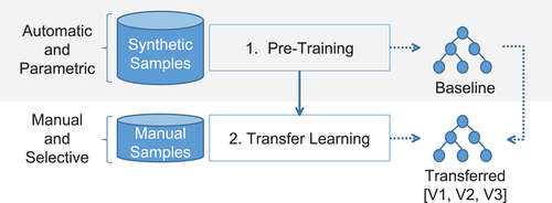
Transfer learning is beneficial in two ways here: i) it requires significantly less data to transfer an existing pre-trained network, and ii) it simplified labelling efforts, as one label could be used for a set of multiple windows, thereby spanning a longer time frame that was more convenient to label, in contrast to requiring a label for each window.

The method we developed successfully applied transfer learning to a pre-trained neural network. Before the transfer learning approach is discussed, we explain both the used windowed time-series data and the network architecture.

3.1. Pre-processing and pre-training

For this work, we used the same pre-processing as in the previous work and its pre-trained neural network model. The pre-processing was done entirely with the rsdtlib library Zitzlsberger et al. (2023) that allows different parameters for the windowed time-series construction. In the following, we summarize the key aspects of the pre-processing and the pre-trained neural network model as necessary.

The analysis of urban changes was done on a window by window basis. Windows were defined with a period of 6 months ($\mathrm{\Delta }$) for Sentinel 1 and 2 missions, as also used in our current work. These windows were created with the two-step procedure illustrated in Figure 2. First, each observation mode (optical multispectral and SAR ascending or descending orbit direction) was temporally stacked to interpolate the missing pixels. Missing pixels occurred for masked clouds, areas out of swath, or if only one mode was updated at one point in time. For simplicity, we allowed the combination of multiple observations within a step $\mathrm{\Delta }$ (2 days for Sentinel 1 and 2). This reduced redundancies that can occur when swaths overlap spatially in a short time period. The choice of using a two-day period provided a compromise between the detection of long-term (urban) changes and the reduction of (redundant) observations, which resulted in only minimal information loss. The result was a stack of observations with combined modes that at every observation time point contained an approximate state of the Earth’s surface (assembly). The temporal stack was further tiled into patches. In a second step, windows of a defined duration $\mathrm{\Delta }$ were created, each with a stride of one observation ($\rho$). The result was a set of windows $w_{i,j}^t\in {\mathbb{W}}_{i,j}$ for tiles with coordinates $(i,j)$ for a selected AoI, starting at an observation time $t$. Coordinates $i$ and $j$ denote the tile coordinates in the $y$ and $x$ dimensions, accordingly. To avoid degradation in prediction performance, a minimum number of observations $\omega$ had to be present. Windows with less than $\omega$ observations were discarded. In addition, an upper bound $\omega$ to the number of observations exists, which is a result of the window duration $\mathrm{\Delta }$ and step $\mathrm{\Delta }$ ($\mathrm{\Omega }\approx \frac{\mathrm{\Delta }}{\delta }$). All parameters for the data types and the creation of time-series windows were identical to the pre-training and are summarized in Table 1.

Figure 2. Data preparation in two-steps, using the available observations to build windows ${\mathit{w}}_{i,j}^t\in {\mathbb{W}}_{i,j}$ enumerated for every following observation. The synthetic labels ${\hat{\mathit{y}}}_{i,j}^t$ are only used for pre-training and not for transfer learning.

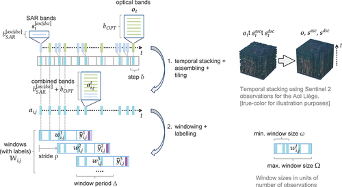
Table 1. All parameters of remote-sensing data and constructed windows used in our work. Data related parameters are bound to Sentinel 1 and 2 sensor characteristics. Window-related parameters are bound to the pre-trained network stage.

	Parameter	Mnemonic	Value
data	$b_{SAR}^{\left[asc|dsc\right]}$	SAR bands	2 (VV+VH)
	$b_{OPT}$	optical bands	13
	$\delta$	step $\left(\frac{\cdot }{\mathrm{o}\mathrm{b}\mathrm{s}\mathrm{e}\mathrm{r}\mathrm{v}\mathrm{a}\mathrm{t}\mathrm{i}\mathrm{o}\mathrm{n}}\right)$	2 days
windows	$\mathrm{\Delta }$	window period	6 months
	$\rho$	stride	1
	$\omega$	min. window size	35
	$\mathrm{\Omega }$	max. window size	92

We built on the aforementioned pre-trained network, which was trained with the synthetic labels ${\hat{\mathit{y}}}_{i,j}^t$ of the AoIs of Rotterdam (the Netherlands) and Limassol (Cyprus). Table 2 summarizes the used data and data sources, and Figure 3 shows the model architecture. The advantage of this approach was that manual labelling was not needed and the resulting trained network converged to a solution. However, despite its demonstrated utility, there were limits to controlling which (urban) changes it detected. False positives existed that denoted urban-related changes due to moving vehicles or containers, reflective surfaces in both optical and radar (Nielsen et al. 2017) data, and arid soil during droughts, for example. Also, because the prediction values were related to the intensity of changes, those changes with a longer duration received higher values than short-term ones. It is therefore desirable to receive a strong response to shorter changes to avoid them being overlooked.

Figure 3. The architecture as inherited from the pre-training stage. In the transfer learning stage, all layers are trained. A multi-modal input is expected (green background: multispectral optical; blue background: SAR in ascending and descending orbit directions). Hyper-parameters of the respective layers are detailed in the table on the right.

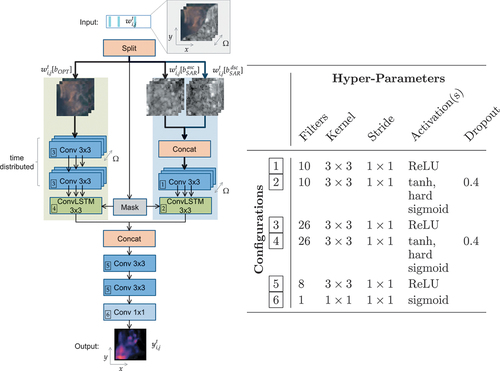
Table 2. Used AoIs, the covered area, and the number of their available observations, with removed ones in parenthesis. Only level 1 products are used. AoIs in grey were used for pre-training only.

		SAR observations		Optical multispectral		Area
	Site	(ascending & descending)		observations		($\mathrm{k}{\mathrm{m}}^2$)
	Rotterdam	1,603 (−4)		278 (−10)		523.6
Sentinel 1 & 2 2017–2021	Limassol	468 (−0)		407 (−35)		576.2
	Liège	1,040 (−0)		332 (−35)		507.7
	Sources		SAR: 10 m/pixel, Sentinel 1, SENTINEL1_IW_[ASC|DSC]
			Optical: 10 m/pixel, Sentinel 2, L1C

The main building blocks of the architecture were two-dimensional convolution (LeCun et al. 1989) and convolutional Long Short-Term Memory (Hochreiter and Schmidhuber 1997) (convLSTM (Shi et al. 2015)) layers to identify spatial and spatio-temporal features, respectively. The synthetic labels ${\hat{\mathit{y}}}_{i,j}^t$ were not used in our current work and can be ignored. We refer to the pre-trained network, more precisely its state, as baseline. This network predicted for each window $w_{i,j}^t$ the urban changes $y_{i,j}^t$ that happened within its duration $\mathrm{\Delta }$. The network did not apply a softmax (Bridle 1989) activation at the end but only a sigmoid activation (Han and Claudio 1995) since the distinction of only two classes (change and no-change) was needed. Hence, the outputs (predictions) for each pixel were continuous values that represent the probability of a change $p_{change}\in [0,1]$. Conversely, the probability of no-change is $p_{no-change}1-p_{change}$ for each pixel.

For this work, we continued training the pre-trained network to optimize for a different AoI. We used transfer learning over a random set of partially overlapping windows in each tile to cover the time frame of 2017–2020, instead of just using individual six-month windows. For each tile, we created an approximated binary ground truth ${\tilde{\mathit{y}}}_{i,j}$ which highlights changes irrespective of their duration.

3.2. Transfer learning

The new binary ground truth data was manually created for a small number of samples from the final target area to guide the transfer learning process. This labelling was the only manual step and was kept minimal¹ to demonstrate the efficacy of our approach. A description of the ground truth labelling and transfer learning process follows.

3.2.1. Ground truth

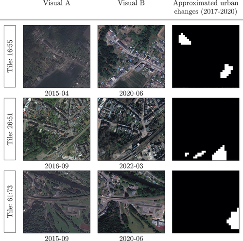
The manual labelling process to generate the ground truth ${\tilde{\mathit{y}}}_{i,j}$ for every tile was guided by visual inspection of very-high resolution historic satellite and aerial imagery from Google Earth. A random set of tiles from the target AoI Liège was selected for labelling. These tiles were used for training, validation, and testing sets during transfer learning. Due to the scarcity of samples, it was not possible to narrow down the time frame of changes precisely. Hence, we considered longer time frames of multiple years instead of individual windows to maximize the availability of third-party sources. Pixels were attributed with a value of 1.0 if an urban change looked visually likely and 0.0 otherwise. Changes could be any kind of human interaction, such as replacing vegetation with human made objects or vice versa, the construction of new buildings and roads, or their destruction. We also noted modified soil around construction sites to take into consideration the impact on the environment. Changes that were smaller than the sensor resolution were ignored. Due to the higher temporal resolution of our method, we were also able to acknowledge changes that only happened temporarily if visible or indicated in the very-high resolution images, such as the digging of trenches or erection of construction support structures. This labelling was intentionally conservative and any questionable temporary changes or those that were of an unclear extent beyond the selected time frame were not considered. However, temporary changes and impacted area around construction sites were treated as a change if backed by the available visual data. Figure 4 shows three examples using two visual samples and the created ground truths. Depending on the exact location, a varying number of five to seven historical observations were available and screened within the selected AoI.

Figure 4. At least two historic Google Earth™ very-high resolution images ‘near’ the beginning of 2017 (left) and the end of 2020 (middle) are used to approximate the ground truth ($32\times 32$ pixel) for urban changes (right).

Samples were assigned to a combined training and validation (trainval) set, and a fixed testing set. We attempted different transfers of the pre-trained model and randomly drew training and validation samples from trainval, with the different validation sets being disjunct (non-exhaustive cross validation). Across all transfers, the testing set remained fixed. In addition, we did not consider tiles that had excessively large and homogeneous changes and skipped them when randomly selecting tiles. This was to avoid biasing the transfer learning process with, for example, extensive open-pit mines or timely concurrent constructions of large groups of houses. These would contribute to an increased number of changed pixels with very similar (yet identical) change patterns. Smaller changes with different patterns would be underrepresented and less likely learned. Instead, we used tiles with a diverse representation of changes that made up no more than 10% of the entire tile.

3.2.2. Training process

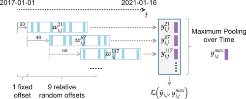
The training process of the pre-training stage was modified for the transfer learning stage, as detailed in algorithm 1. For each tile, we inferred predictions $y_{i,j}^t$ over all windows $w_{i,j}^t\in {\mathbb{W}}_{i,j}$. All of these predictions were combined by a maximum operation to $y_{i,j}^{max}$. This realized a Maximum Pooling over Time Collobert et al. (2011), i.e. each pixel value in the final overall prediction stemmed from at least one window. The resulting $y_{i,j}^{max}$ was subject to the loss function $\mathcal{L}$ against the ground truth ${\tilde{\mathit{y}}}_{i,j}$.

This had two downsides: i) it was not possible to provide information about which subset of windows a specific change happens in, and ii) changes were not labelled in a way that considers different intensities, i.e. whether they happen over a shorter or longer time. The advantage, however, was the reduction of the required manual work: a minimum of only two samples were needed, one from close to beginning and the end of the considered multi-year period. In turn, this reduced the resource needs for providing labelled data drastically, considering that hundreds of windows exist in such a time range. As we show later in section 6.4, there was no breakdown of temporal coherence in the predictions over time, contrary to the expected downside of not being able to provide information about when changes happen. For the discussion of the results of our work, it should be stressed that this labelling process is error-prone and only acts as a tool to narrow down the final solution with the least amount of manual work. It is self-evident that using more rigorous labelling and more samples from different sources can lead to better results. We have intentionally demonstrated a minimal effort case to emphasize its utility.

Table

Algorithm 1 Multi-window training step for transfer learning. Instead of training with one window, multiple windows are aggregated into a set that is considered for each training step.
Input: ${\mathbb{W}}_{i,j}$: windows for tile $(i,j)$, ${\tilde{y}}_{i,j}$: manual label for tile $(i,j)$, ${\theta }_s$: model parameters at training step $s$, $f_{\mathrm{\Delta }}$: forwardpropagation with parameters $\mathrm{\Delta }$
Output: ${\theta }_{s+1}$: model parameters for next training step $s+1$, $\mathcal{L}$: loss for ${\mathbb{W}}_{i,j}$
1: $y_{i,j}^{max}\leftarrow \mathbf{0}$
2: ${\theta }_s\leftarrow$ model parameters at training step $s$
3: for all $w_{i,j}^t\in {\mathbb{W}}_{i,j}$ do
4: $y_{i,j}^t=f_{{\theta }_s}(w_{i,j}^t)$ // forward propagation
5: $y_{i,j}^{max}=max(y_{i,j}^{max},y_{i,j}^t)$ // element-wise maximum
6: end for
7: ${\theta }_{s+1}\leftarrow {\theta }_s-\alpha {\mathrm{\nabla }}_{{\theta }_s}\mathcal{L}({\tilde{\mathit{y}}}_{i,j},y_{i,j}^{max})$ // back-propagation with stochastic gradient descent (SGD), learning rate $\alpha$
8: return ${\theta }_{s+1}$, $\mathcal{L}({\tilde{\mathit{y}}}_{i,j},y_{i,j}^{max})$

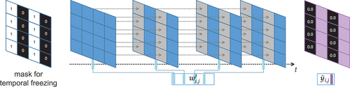
Considering the limited amount of training data, we applied different random augmentation techniques to avoid overfitting whilst reducing the variance of the trained model and improving its generalization. Tiles and all their enclosed windows were flipped horizontally and rotated in 90 degree increments. Furthermore, we added a novel augmentation technique to narrow the perceptive field so that more attention was paid to each pixel’s spectral and radar responses. As shown in Figure 5, a stripe mask with a one pixel width was applied. The mask indicated for which pixel only the first observation was replicated throughout the window. We call this temporal freezing and it was applied for the masked pixels (set to one) by broadcasting the state of each pixel and channel/band from the first instance throughout the entire window’s time series. This created a ‘temporal comb’ filter on the expected predictions as masked columns were not subject to any change. Hence, the invariance over time had to produce values 0.0 in the prediction. All three augmentation strategies increased the training and validation datasets by a factor of 16: a factor of two for horizontal flipping, four for rotation and two for adding or not adding a temporal comb filter.

Figure 5. Temporal freezing using a stripe mask that replicates the first observation in window $w_{i,j}^t$ to all following ones (in grey). The expected ground truth must therefore be zeroed for the masked and temporally frozen pixels in ${\tilde{y}}_{i,j}$ due to no change occurring.

4. Study area

For the underlying work, we used the AoI Liège with an area of approximately 508 $\mathrm{k}{\mathrm{m}}^2$ (before tiling). This area provided a variety of urban and rural areas, with agricultural land, industrial zones, and water bodies. The selected area is topographically comprised of elevation differences carved by rivers in the outskirts of the low mountain range of Eifel in the south-east. A flat in the north-west is mostly used for farming. The city of Liège lies in the centre of the selected AoI and has a size of ca. 69 $\mathrm{k}{\mathrm{m}}^2$ with a population of ca. 195.000. It also exhibited different observation patterns for the sites at Rotterdam and Limassol that were used for pre-training.

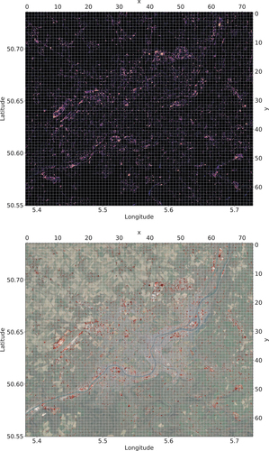
As input data, all available level 1 Sentinel 1 and Sentinel 2 observations were considered, except for 35 optical ones that were removed due to having cloud coverage of over 80% or co-registration errors (see Table 2). The area was tiled into $32\times 32$ pixel patches, using a resolution of 10 m per pixel. 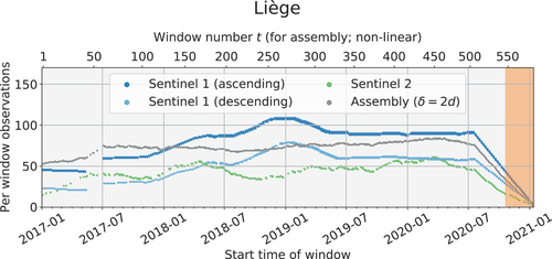The grid of tiles and the location of the AoI are illustrated in Figure 6, with a total of $67\times 74$ tiles. As shown in Figure 7, we considered the entire time frame from the start of 2017 up to mid-January 2021 where sufficient historic Google Earth very-high resolution images were available. However, we skipped the first 20 windows to avoid optical observations having no values due to the applied cloud masks in the stacking process. Hence, windows effectively started with the beginning of March 2017, from when on all pixels had proper values in each observation. This eased the training of the neural network as corner cases of pixels without values (or zero padded values) did not need to be learned, which in turn reduced the need for increased network capacity. Also, the impact on missing urban changes was low as such changes are less likely during the winter. The last considered window started mid-2020, as windows starting later would have extended into 2021 due to their 6-month duration ($\mathrm{\Delta }$).

Figure 6. Tiles for AoI Liège. The blue tiles are used for training and validation (152 in total). The 32 tiles in orange are used for testing. Geographic coordinates are in EPSG:4326 and tile coordinates are in $(y,x)$ dimensions, covering an area of approximately 508 $\mathrm{k}{\mathrm{m}}^2$. Background image $\copyright$ 2019/20 Google Earth, for reference only.

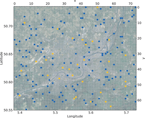
Figure 7. Windows and their observations. In our work, we combine Sentinel 1 (blue) and 2 (green) observations in a two day ($\delta =2\mathrm{d}\mathrm{a}\mathrm{y}\mathrm{s}$) interval (grey). Highlighted in orange and discarded are windows with less than 35 ($\omega$) observations.

A total of 184 randomly chosen tiles of the AoI of Liège were selected and labelled − 152 were assigned to the trainval and 32 to the testing set. Figure 6 shows the selected tiles in blue and orange, respectively. Three different training and validation set pairs were randomly drawn from the trainval, with 120 samples each for training and 32 for validation. These three pairs had disjunctive validation sets and were used for transfer learning of the baseline to receive the transferred model variants V1, V2, and V3. Augmentation was applied during the training to both the training and validation sets, due to which we received a total of 2,432 (1,920/512) samples when training each variant.

5. Implementation

The method we developed was implemented on the Karolina GPU cluster² at IT4Innovations. One compute node was utilized for training, which contained eight NVIDIA A100 GPUs, each with 40 GB of memory. The original training environment with Tensorflow (2.7), including Keras, and Horovod (Sergeev and Del Balso 2018) (0.23.0) was unchanged. However, the training process was extended to use the previously described training and validation sets from section 4 and their respective windows. The training configuration remained identical to that of pre-training, which uses a synchronous SGD (Chen et al. 2016; Zinkevich et al. 2010) with a momentum of 0.8 and a fixed learning rate $\alpha$. We only increased $\alpha$ to 0.008 as the pre-training was done on four GPUs instead of eight. We also continued to use the same Tanimoto loss with complement (Diakogiannis et al. 2020) and ignored the predictions on the border pixels (dead area), so only the centre $30\times 30$ pixels of each tile were considered for the loss. It is a general problem of tiled data with convolutional networks that pixels towards the border show higher errors (Huang et al. 2018, 2019; Isensee et al. 2021; Reina et al. 2020). This can be mitigated by using larger tiles that allow the removal of broader borders or overlapping tiles. In our case, the errors near the borders increased as prediction values were boosted by the model to meet the binary ground truth. However, we did not extend the dead area to avoid losing too much label information and empirically only observed very few cases that would have required a larger dead area. As such, considering the central $30\times 30$ pixels was a viable compromise.

Transfer learning was applied to the entire pre-trained model, and none of the layers was frozen. This was due to the shallow nature of the used network architecture. For deeper networks, layers closer to the input extract more general features compared to the ones towards the output, which are more specialized (Yosinski et al. 2014). In such cases, freezing the layers on the input side would be a viable method for transfer learning, as it only trains the specialized layers and reuses the general ones. In our shallow network architecture, the layers are less likely to develop a distinguishable generalization/specialization pattern. Our case benefited from transfer learning by being able to start off with a well functioning solution for spatio-temporal data, and by being able to continue training with less precise temporal information but a more concise definition of the (urban) changes to detect.

The extension of training data to a set of windowed deep-temporal data samples instead of individual windows proved challenging in terms of memory utilization. In our previous work, as well as in Isensee et al. (2021); Roth et al. (2018), the selected tile size was based on the available GPU memory. With the transfer learning of multiple windows at once, the challenges due to limited memory needed to be reconsidered. Not only the tile size but also the number of windows simultaneously used for training should be determined by the available memory. We mitigated these problems by using the adapted data and memory management system shown in Figure 8. This comprised two aspects: batch size trade-off and selection of windows.

Figure 8. Data and Memory Management. Each training sample (tile) consists of 10 randomly selected windows.

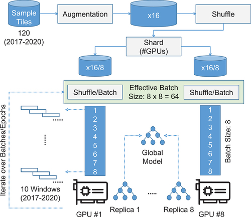
5.1. Batch size trade-off

As Figure 8 shows, training samples were derived from the manually labelled sample tiles (120) with augmentation applied ($\times 16$). This augmented set was shuffled and an equally sized subset (shard) was assigned to each GPU ($\times 16/8$). These shards stayed fixed throughout the training session, that is, each GPU trained the same subset of samples (augmented tiles) over all epochs. The network was trained for each augmented sample. This defines an iterative process for which a maximum over all individual predictions is computed. As a result, the network was trained over all used windows for each training step, which required a large amount of memory. Due to the large size of individual samples, with regard to their windows, the batch sizes had to be kept small. We used a batch size of eight for each of the eight GPUs involved. Each GPU trained a replica of the same model. The replicas were synchronized after every training step with synchronous SGD to retrieve a global model. This resulted in an effective batch size of 64 with a total memory consumption of eight times 35 GB (an approximate total of 280 GB). Larger batch sizes resulted in running out of memory, and smaller batch sizes were problematic due to higher loss noise and convergence problems.

5.2. Selection of windows

For every training sample, we considered all windows starting in the time period ranging from the beginning of 2017 up to mid-2020. For the AoI of Liège, there were 540 overlapping windows $t\in [1,540]$, each containing between 35 and 82 observations, as shown in Figure 7. Not all windows fit into the GPU memory at once, which was mitigated by randomly selecting only a subset of partially overlapping windows and ensuring they cover the entire four-year time span. Figure 9 shows an example of one random selection. The first window always started at $t=21$ as not every pixel had a value at $t\in [1,20]$ due to the use of cloud masks within the temporal stacking process. The subsequent nine windows were drawn from uniform random relative offsets in the range of $[45,55]$. These values were chosen so that the expected overall span across all selected windows ended between the second half of 2020 and beginning of 2021. This was done for every tile (training sample) in each batch independently to avoid similar patterns appearing in selected windows within each batch. Effectively, every training sample across all batches contained 10 windows with varying, non-identical temporal coverage that contributed to the generalization of the network. The random selection of windows serves the same purpose as augmentation by reducing the variance of the trained model and improving its generalization. The requirement of partial overlap avoids observation gaps and the training always considers all observations in the multi-year time span, without information loss (except for the start and end). The initial offset and the variance of relative window offsets result in coverage starting in spring 2017 and ending around autumn 2020. This decision was deliberate as the least amount of changes are expected during winter. It minimized the error resulting in differences in the period of the ground truth and the real temporal coverage during training.

Figure 9. Ten Windows selected randomly from across the time period spanning the beginning of 2017 until early 2021. Every window is subject to forward propagation but back-propagation (i.e. training) is only carried out over the maximum of all predictions $y_{i,j}^{max}$.

6. Results

Three models were trained using transfer learning with different training and validation datasets to receive the transferred model variants V1, V2, and V3. In the following, we discuss the training and validation losses and provide a quantitative and qualitative analysis. In addition, we also combine the three transferred model outputs (ensemble) to retrieve only changes that were agreed on by all models. Finally, the limitations of our method are discussed.

6.1. Training and validation losses

The training and validation losses for the transfer of the three variants are plotted in Figure 10. Mean losses across all GPU data partitions are plotted. Additionally, an ab initio training of the same network architecture was carried out, which trains ERCNN-DRS from scratch without the use of the pre-trained model.

Figure 10. Loss values over epochs for all three transferred and ab initio variants. The transfer training losses are represented by the blue curve, and the validation losses by the orange curve. The orange dashed lines show the best epochs based on validation data. Analogues for the ab initio variants in grey colors.

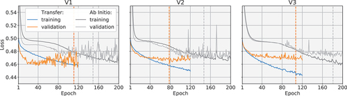
The best epochs for the variant models V1, V2, and V3 were selected based on minimal validation loss. These were, epoch 111 for V1, epoch 78 for V2 and epoch 107 for V3. The same was done for the ab initio cases, which resulted in the selection of epoch 149, 147, and 181 for V1, V2, and V3, respectively.

Comparing the transfer to the ab initio training shows a clear advantage in time-to-solution as well as a lower minimum of the loss value means ($\approx -0.005$) for all transfer cases. The ab initio training sessions took 36 h to reach epoch 200, whereas the transfers took 21:30 h to reach epoch 120, both with the same training configuration and datasets.

In the following, the per-tile predictions of the three individually transferred models at epochs 111, 78 and 107 are referred to as $y_{i,j}^{V1}$, $y_{i,j}^{V2}$, and $y_{i,j}^{V3}$, respectively. They reflect a maximum of predictions over all windows, so that

$y_{i,j}^{V1}:=max\{f_{V1}(w_{i,j}^t):w_{i,j}^t\in {\mathbb{W}}_{i,j}\}$

with element-wise $max$ over the two-dimensional prediction outputs. The forward propagation $f_{V1}(\cdot )$ uses the trained parameters of V1, accordingly for $y_{i,j}^{V2}$ and $y_{i,j}^{V3}$.

6.2. Quantitative analysis

To quantify improvements to the models, the binary classification metrics summarized in Table 3 were used for each trained model, covering all pixels in the training, validation, and testing sets. The ground truth is by definition binary, whereas the predictions of the neural networks are continuous values. Hence, the latter were subject to thresholds when computing the metrics. In the following, the receiver operating characteristic (ROC) and precision recall (PR) curves, Cohen’s kappa with different thresholds, and basic metrics like precision, recall, and F1-score for selected thresholds are discussed. Neither training nor validation sets were augmented when retrieving the quantitative results.

Table 3. The summary of used metrics with their descriptions and derivations.

Metric	Description/Derivation
True Positive ($TP$)	A change is correctly predicted as such
True Negative ($TN$)	A no-change is correctly predicted as such
False Positive ($FP$)	A no-change was predicted wrongly as a change
False Negative ($FN$)	A change was predicted wrongly as a no-change
True Positive Rate ($TPR$), Recall	$\frac{TP}{TP+FN}$
False Positive Rate ($FPR$)	$\frac{FP}{FP+TNP}$
Precision	$\frac{TP}{TP+FP}$
F1-Score ($F_1$)	$\frac{2TP}{2TP+FP+FN}$
Cohen’s Kappa ($\kappa$)	$\frac{2\left(TPTN-FPFN\right)}{\left(TP+FP\right)\left(FP+TN\right)\left(TP+FN\right)\left(FN+TN\right)}$

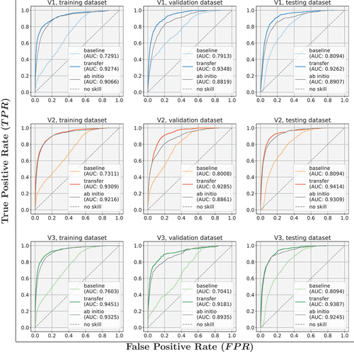
ROC curves are common in machine learning for binary classifiers (Majnik and Bosnić 2013). They show the true positive rate ($TPR$) versus the false-positive rate $FPR$ using varying thresholds. The ROC curves and their area under the curve (AUC) in Figure 11 show an improvement in prediction across all the variants and datasets, when compared to the baseline. The performance of the baseline was lower in all cases. It is also worth noting that the ab initio variants fell short of achieving the performance of their transferred counterparts. For segmentation-like problems like those tackled in our work, the pixel-related imbalance of background (no-change) and foreground (change) classes rendered ROC curves less useful. No-changes were more prevalent and to a greater extent, whereas changes happened less often in some hotspots spanning over fewer windows.

Figure 11. ROC curves for all three transfer and ab initio variants, showing training, validation, and testing datasets separately with their AUC. The grey dashed line is a model without any skill (i.e. best guessing).

PR curves (Raghavan, Bollmann, and Jung 1989) can give more detailed insights compared to ROC curves for skewed datasets (Davis and Goadrich 2006). They plot the precision and recall values for different thresholds of the prediction values. Figure 12 shows the PR curves for the three variants per dataset. For all datasets, the AUC improved significantly for the transferred variants when compared to the baseline. In particular for the fixed testing set, all three transferred models were improved by at least a factor of four. Even though the ab initio variants were better than the baseline (apart from one case, the V2, validation dataset), they performed worse than the transferred variants.

Figure 12. PR curves for all three transfer and ab initio variants, showing training, validation, and testing datasets separately with their AUC. The grey dashed line is a model without any skill (i.e. best guessing).

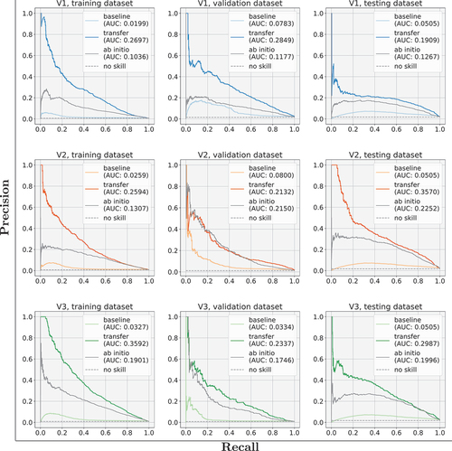
We would like to stress here that we show an end-to-end result with different errors impacting the overall performance. We discuss them in detail in section 6.4. In addition, the baseline was originally trained with a different objective, therefore its performance was, as expected, quite low compared to a (semi-)heterogeneous transfer learning setting.

Cohen’s Kappa (Cohen 1960) is a measure of the agreement of two raters and was applied in this work for the two classes of change and no-change. Since Kappa expects binary values, we studied it with different thresholds applied to the prediction values. Figure 13 shows the Kappa values of the three variants and datasets separately. It is clearly visible that for the baseline the best threshold was about $0.4(\pm 0.05)$ whereas for the transferred models it shifted towards $0.8(\pm 0.15)$. This is due to the labelled ground truth having been binary only, irrespective of the change duration, whereas the pre-trained network provided values proportional to the change duration. The ab initio variants again provided a better performance compared to the baseline but, except for one case (V2, validation dataset), did not reach the same level as the transferred variants.

Figure 13. Value of Cohen’s Kappa $\kappa$ (y-axis) for all three transfer and ab initio variants, showing training, validation, and testing datasets separately. Prediction values are subject to a threshold shown on the x-axis.

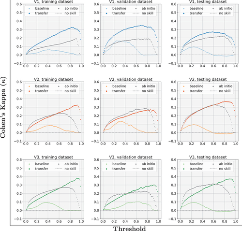
A slight negative kappa occurred for larger thresholds with the baseline testing dataset. A kappa value of zero indicates no skill, i.e. best guessing, and a kappa value below zero indicates that the predicted values are in reverse. However, here the values below zero were minute, and the size of the testing set was small. That switch for certain thresholds can therefore be attributed to outliers. For all transferred models and datasets, the kappa value noticeably improved. Similar to the PR curves, different errors lowered the performance and a detailed analysis of absolute values would not have been meaningful. Instead, we show the relative improvements to demonstrate the efficacy of our method.

In Table 4 the metrics of precision, recall, and F1-score for both classes with their averages are listed. Metrics are shown for the baseline and the three transferred models, separately for each of the three datasets. The baseline results varied due to the changing training and validation datasets across the different transferred variants. For testing, these were identical for the baseline model. The best thresholds from the Kappa evaluation were used for the metrics, which were 0.4 for the baseline and 0.8 for the transferred models. Due to the immanent imbalance of classes, the background class (no-change) dominated and did not change to the same amount as the foreground one. Differences in precision, recall, and F1-score became more visible when considering the foreground class (change). For the no-change class, these metrics are back to front, and hence foreground and background classes are exchanged, compared to Table 3. In all cases, the scores improved from the baseline to the transferred variants.

Table 4. Precision, recall, and F1-scores of the pre-trained baseline and the three transferred models. A threshold of 0.4 is used for the former, 0.8 for the latter. The number of pixels for the respective classes in the ground truth is shown for each configuration.

		Training				Validation				Testing
		Precision	Recall	F1-Score	Pixels	Precision	Recall	F1-Score	Pixels	Precision	Recall	F1-Score	Pixels
V1	Baseline
	No-change	0.99	0.99	0.99	122,052	0.99	0.99	0.99	32,281	0.98	0.95	0.97	32,193
	Change	0.05	0.11	0.07	828	0.16	0.18	0.17	487	0.05	0.17	0.08	575
	Average	0.52	0.55	0.53	122,880	0.57	0.58	0.58	32,768	0.52	0.56	0.52	32,768
	Transfer
	No-change	1.00	0.99	0.99	122,052	0.99	0.99	0.99	32,281	0.99	0.98	0.98	32,193
	Change	0.25	0.45	0.32	828	0.35	0.32	0.33	487	0.22	0.34	0.27	575
	Average	0.62	0.72	0.66	122,880	0.67	0.65	0.66	32,768	0.60	0.66	0.62	32,768
V2	Baseline
	No-change	0.99	0.98	0.99	121,957	0.99	0.99	0.99	32,376	0.98	0.95	0.97	32,193
	Change	0.07	0.15	0.09	923	0.18	0.10	0.13	392	0.05	0.17	0.08	575
	Average	0.53	0.57	0.54	122,880	0.59	0.55	0.56	32,768	0.52	0.56	0.52	32,768
	Transfer
	No-change	1.00	0.99	0.99	121,957	0.99	0.99	0.99	32,376	0.99	0.98	0.99	32,193
	Change	0.22	0.44	0.29	923	0.23	0.31	0.27	392	0.31	0.51	0.39	575
	Average	0.61	0.72	0.64	122,880	0.61	0.65	0.63	32,768	0.65	0.74	0.69	32,768
V3	Baseline
	No-change	0.99	0.99	0.99	121,829	0.99	0.98	0.99	32,504	0.98	0.95	0.97	32,193
	Change	0.08	0.14	0.10	1051	0.06	0.15	0.08	264	0.05	0.17	0.08	575
	Average	0.52	0.56	0.55	122,880	0.53	0.56	0.54	32,768	0.52	0.56	0.52	32,768
	Transfer
	No-change	1.00	0.99	0.99	121,829	1.00	0.99	0.99	32,504	0.99	0.98	0.98	32,193
	Change	0.25	0.56	0.34	1051	0.22	0.43	0.29	264	0.28	0.53	0.37	575
	Average	0.62	0.77	0.67	122,880	0.61	0.71	0.64	32,768	0.64	0.75	0.68	32,768

Since there were three different transferred models, each trained with a different split of training and validation data, they could be combined to further improve the overall result. This followed the bagging (bootstrap aggregating) Breiman (1996) methodology. Their predictions passed through a sigmoid activation that allowed them to combine with

$y_{i,j}^{V1+V2}:=\sqrt{y_{i,j}^{V1}\cdot y_{i,j}^{V2}},y_{i,j}^{V2+V3}:=\sqrt{y_{i,j}^{V2}\cdot y_{i,j}^{V3}},y_{i,j}^{V1+V3}:=\sqrt{y_{i,j}^{V1}\cdot y_{i,j}^{V3}},$

$\mathrm{a}\mathrm{n}\mathrm{d}{y}_{i,j}^C:=\sqrt[3]{y_{i,j}^{V1}\cdot y_{i,j}^{V2}\cdot y_{i,j}^{V3}},$

where the used operations were the Hadamard multiplication and the square/cube root. The latter one, denoted as combined, was predominantly used in this work; the former three were provided only for completeness. This combination was used to acknowledge only prediction values that were of high confidence from all three model variants. Misclassification was likely an error of individual models, hence the prediction of the other models was not likely to have had the same pattern of misclassification and instead would predict values closer to zero. The combination then attenuates the misclassification. Systemic misclassifications cannot be reduced through this approach but are more likely a result of incorrect labelling or overly small amounts of samples. Both can easily be corrected by labelling more samples or ensuring that there are higher-quality labels.

Figure 14 shows the ROC, PR, and Kappa plots for the combined model output $y_{i,j}^C$. Since the training and validation dataset results cannot be shown separately, the results are based on the entire trainval dataset. A comparison of the models V1, V2, and V3 was possible with the testing dataset results that are also shown. Even though this combined output was rather conservative, it was close to the best of the transferred models. This suggests that there is no degradation and a sufficient overlap of predictions close to the ground truth exists. Also, the metrics for precision, recall, and F1-score were high, even though they did not equal the best results from the individual models. The metrics are shown in Table 5 as compared to the baseline. It is also visible that precision and recall were more balanced in the combined output. In most cases, the precision metrics for all models (except for the validation datasets for V1 and V2) were smaller than their recall counterparts. This originated from the higher number of false positives, which was expected since the ground truth labels were only derived from changes that were visible from a few very-high resolution samples. Other changes that happened in between were not sufficiently labelled as such.

Figure 14. ROC, PR, and $\kappa$ for baseline and the four combined transferred models, showing both training and validation (trainval), and testing datasets.

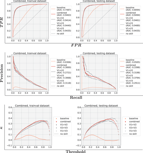
Table 5. Precision, recall, and F1-scores of the pre-trained baseline and the combined transferred models. A threshold of 0.4 is used for the former, 0.8 for the latter. The number of pixels for the respective class in the ground truth is shown for each configuration.

	Training/Validation				Testing
	Precision	Recall	F1-Score	Pixels	Precision	Recall	F1-Score	Pixels
Baseline
No-change	0.99	0.99	0.99	154,333	0.98	0.95	0.97	32,193
Change	0.08	0.14	0.10	1315	0.05	0.17	0.08	575
Average	0.53	0.56	0.54	155,648	0.52	0.56	0.52	32,768
Combined
No-change	0.99	0.99	0.99	154,333	0.99	0.99	0.99	32,193
Change	0.35	0.37	0.36	1315	0.36	0.40	0.38	575
Average	0.67	0.68	0.68	155,648	0.68	0.69	0.68	32,768

6.3. Qualitative analysis

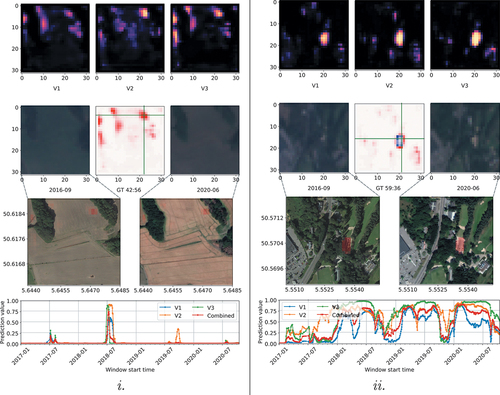
Figure 15 shows four samples with different urban change patterns. For each sample, the predictions $y_{i,j}^{V1}$, $y_{i,j}^{V2}$, and $y_{i,j}^{V3}$ are displayed in the top row. Dark pixels show a low probability of change, while brighter pixels show a higher probability. The second and third rows show two visual representations using true colour Sentinel 2 and Google Earth very-high resolution images, respectively. The representations were limited by the availability of the latter, which were used for labelling and detailed inspection. Conversely, Sentinel 2 images were not sufficient to identify urban changes manually, but demonstrate the spatial resolution the neural network operates on. Superimposed in red on the very-high resolution images are the combined predictions $y_{i,j}^C$. The middle of the second row shows the tile’s coordinates and the difference of its ground truth (GT) to the combined prediction $y_{i,j}^C$. Red colouration denotes false positives and blue false negatives. Colours close to white are true positives/negatives. One pixel is selected by the green cross hair with its windowed prediction values plotted over time in the bottom chart. The plots show all three transferred model variant outputs and their combination.

Figure 15. Four different examples (tiles) demonstrating urban changes.

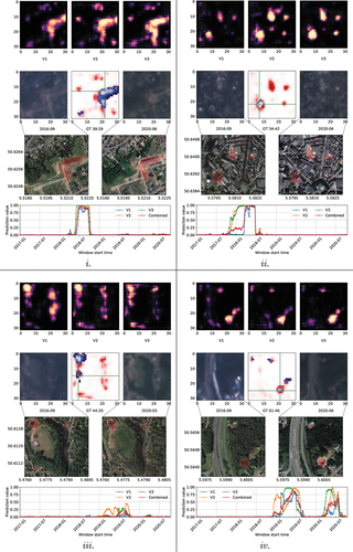
Example i. in Figure 15 shows a large construction area for housing (middle, right). The construction of the house selected with the green cross hair occurred in 2018, as can be derived from the time plot. All three model predictions show very similar value changes and so does their combination. A more complex urban change pattern is shown in example ii. It shows the destruction of a building and a subsequent new construction (bottom left) in a densely populated area in 2017/18. The transferred variants show a different response over time for this very change. Variants V2 and V3 had already identified changes in 2017, whereas V1 only did so in 2018. This is a result of the networks extracting different features to identify urban changes. Also, visible here is the effect of combining the predictions from the three models while still acknowledging the early changes from the majority, despite V1 having values close to zero. In example iii. a large construction at the top left and some small-scale destruction in the middle left are visible. The time plots are for the destruction of a stall with a smaller footprint. Values are different for the different transferred variants due to the complex patterns caused by the destruction, leaving behind a concrete base. Again, the networks identified different patterns as a change that happened at different times during the destruction process. Deforestation and construction of a building is visible in example iv. towards the bottom right. Three other smaller constructions and changes are also observable. The selected change happened in two intervals, in 2019 and early 2020.

A result of the combined model applied to the entire selected AoI of Liège in the time frame 2017–2020 is shown in Figure A1 in Appendix A.

6.4. Limitations

Some limitations arose from our method being demonstrated in an end-to-end scenario. Because level 1 observations were used ‘as is’, the ground truths were approximated with only a few third-party samples, and no other auxiliary information was added, the effective errors were high. They mostly stemmed from three different origins. First, all level 1 observations were used with no manual filtering applied, except for the application of cloud masks provided by Sentinel Hub. As a result, the prediction quality degraded where fewer observations were available in a window or clouds were not properly removed. Other atmospheric problems further added to this. Second, the maximum sensor resolution of 10 m/pixel was too coarse to distinguish small objects like vehicles, containers, or even smaller buildings. In addition, the mixed pixel problem was quite significant at this resolution. Third, our labelling process was only approximate. The extent of changes (delimitation) could have been over- or under-estimated, and the distinction between changes might not have been coherent. Also, there was no information on the intensity (or probability) of changes, and labels were strictly binary.

Figure 16 shows examples of false positives. Example i. depicts farmland where the effect of a short-term drought in Western Europe in the summer of 2018 became noticeable. An erroneous detection resulted from arid soil as it is hard to distinguish from construction sites. An area on the top right appeared very briefly in mid-2018 on the timeline. All three models misclassified it, and so even the combined model was incorrect. Effects of moving vehicles on a car park are shown in example ii. The selected area of the car park was extended in mid-2017, and the movement of vehicles lead to false positives due to the mixed pixel problem stemming from the lower sensor resolution. This is apparent when comparing the true colour Sentinel 2 images in the left and right images on the second row. Another frequently used car park can be found in Figure 15 example ii. near the top centre, which also led to false positives. In addition, strong reflective objects like white rooftops on buildings, photovoltaic panels, or metal objects can saturate the sensors easily. This is visible in Figure 15 example iii. on the right, where parked cars and the reflective surfaces of the houses across the street combined to increase false positives. Especially V1 was susceptible to this. The combined model attenuates these, but they are still visible as shown in the red false positives in the middle of the second row.

Figure 16. Two different examples (tiles) demonstrating limitations of our method.

As mentioned earlier, pixels towards the border of tiled data show higher errors. Since our pre-trained model was fully convolutional, the tile sizes could be freely changed. For training, however, smaller tiles were mandatory to avoid increasing memory needs. For inference, tiles could usually be larger because batches could become smaller and there is no need for trainable network parameters or synchronizations as the models do not change.

Another limitation arose from the manual labelling, which was constrained to identifying mostly long-term changes. The labelling was error-prone for both the background (no-change) and foreground (change) classes. During labelling for the background class, it was assumed that no change happens at all, which is not always correct. Changes can happen intermittently or do not appear in the few very-high resolution samples, e.g. the digging of trenches, or temporary support construction. Conversely, in the foreground class, changes might be assumed that did not happen to the same extent, e.g. a construction did not involve the entire visibly impacted area. We assumed an equal weight for both classes to allow the same amount of deviation. It would be possible to weigh the foreground classes higher than their background counterparts, resulting in a more sensitive detection, and vice versa.

Our approach further redefined the predictive values. In the original pre-trained model, a change was considered as an intensity value, which is proportional to its duration. For the transferred models, the output was shifted towards a binary output, irrespective of the duration of changes. However, this might be preferred in most cases so that even short-term changes are easily found in the predictions.

7. Conclusion

A foundation to train neural networks for urban change detection with windowed deep-temporal multi-modal remote sensing data was set out in the previous work. However, it lacked the third-party sources to provide enough information to label and verify changes properly. This was especially true when labelling each window individually, which led to the use of automatically created synthetic labels that were noisy and provided limited control of urban change types.

In this work, we have demonstrated a practically feasible way to transfer these networks with a set of deep-temporal time-series windows simultaneously, using only a small number of manually approximated labels. We have shown that transfer learning can improve the aforementioned fully automatically trained networks further and optimize them towards specific urban changes and a different target area. Three different transferred variants were successfully trained independently on different but constrained training sets. Furthermore, a combination of all three predictions provided more conservative results without a significant degradation of the performance and better balanced false-positive and false-negative rates.

We further addressed the challenge of having limited memory to train with large-scale deep-temporal data on current systems. A multi-GPU environment was used to enable the ability to increase the effective batch size to avoid non-convergence and high loss noise. Also, the selection of random but overlapping subsets of windows showed its efficacy by allowing training convergence and maintaining steady predictions over time.

Our methods can help to provide a large-scale automatic urban change monitoring with high temporal resolution. A refinement process requires only low labelling resources and provides a high level of adaptation, which improves the quality of predictions. As we work with level 1 remote sensing data, further improvements are easily possible with higher-quality data sources (e.g. level 2) or more rigorous manual labelling.

CRediT Authorship Contribution Statement

G. Zitzlsberger: Conceptualization, Methodology, Software, Investigation, Data Curation, Writing – Original Draft, Writing – Review & Editing, Visualization, Funding acquisition (90%). M. Podhoranyi: Validation, Writing – Review & Editing (6%). J. Martinovič: Resources, Supervision, Project administration (4%).

Acknowledgements

The authors would like to thank the data providers (ESA, Sentinel Hub and Google) for making the used remote sensing data freely available.

Disclosure statement

No potential conflict of interest was reported by the author(s).

Data Availability statement

The labelled data used in this work and trained network models were made available on Github https://github.com/It4innovations/ERCNN-DRS_urban_change_monitoring/. We also provided collateral information like GeoTIFF files of the prediction outputs and videos to visualize the changes over time.

Additional information

Funding

This research was funded by the IT4Innovations infrastructure, which is supported from the Ministry of Education, Youth and Sports of the Czech Republic through the [e-INFRA CZ (ID:90140)], and via Open Access Grant Competition (OPEN-21-31 and OPEN-25-24).

Notes

1. For our results, we allocated approximately two person days for labelling.

2. https://docs.it4i.cz/karolina/hardware-overview/

Appendix A.

Urban Changes in Liège 2017-2020

Figure A1. Urban changes in Liège 2017–2020 with combined models. The top shows identified urban changes using $y_{i,j}^C$ for every tile with black pixels indicating no change and brighter ones a higher probability of occurred urban changes. The bottom shows the same as red highlights to indicate the changes, using a background image $\copyright$ 2019/20 Google Earth, for reference only.

References

- Andresini, G., A. Appice, D. Ienco, and D. Malerba. 2023. “SENECA: Change Detection in Optical Imagery Using Siamese Networks with Active-Transfer Learning.” Expert Systems with Applications 214:119123. https://doi.org/10.1016/j.eswa.2022.119123.
- Bazzi, H., D. Ienco, N. Baghdadi, M. Zribi, and V. Demarez. 2020. “Distilling Before Refine: Spatio-Temporal Transfer Learning for Mapping Irrigated Areas Using Sentinel-1 Time Series.” IEEE Geoscience and Remote Sensing Letters 17 (11): 1909–1913. https://doi.org/10.1109/LGRS.2019.2960625.
- Benedek, C., and T. Sziranyi. 2008. “A Mixed Markov Model for Change Detection in Aerial Photos with Large Time Differences.” In 2008 19th International Conference on Pattern Recognition, Tampa, FL, USA, 1–4.
- Benedek, C., and T. Sziranyi. 2009. “Change Detection in Optical Aerial Images by a Multilayer Conditional Mixed Markov Model.” IEEE Transactions on Geoscience and Remote Sensing 47 (10): 3416–3430. https://doi.org/10.1109/TGRS.2009.2022633.
- Breiman, L. 1996. “Bagging Predictors.” Machine Learning 24 (2): 123–140. https://doi.org/10.1007/BF00058655.
- Bridle, J. S. 1989. “Training Stochastic Model Recognition Algorithms as Networks Can Lead to Maximum Mutual Information Estimation of Parameters.” In Proceedings of the 2nd International Conference on Neural Information Processing Systems, NIPS’89, 211–217. Cambridge, MA: MIT Press.
- Chen, J., S. Chen, C. Yang, H. Liang, M. Hou, and T. Shi. 2020. “A Comparative Study of Impervious Surface Extraction Using Sentinel-2 Imagery.” European Journal of Remote Sensing 53 (1): 274–292. https://doi.org/10.1080/22797254.2020.1820383.
- Chen, J., R. Monga, S. Bengio, and R. Jozefowicz. 2016. “Revisiting Distributed Synchronous SGD.” In Workshop Track of the International Conference on Learning Representations, ICLR, San Juan, Puerto Rico, publications/ps/chen_2016_iclr.ps.gz.
- Chen, H., and Z. Shi. 2020. “A Spatial-Temporal Attention-Based Method and a New Dataset for Remote Sensing Image Change Detection.” Remote Sensing 12 (10): 1662. https://doi.org/10.3390/rs12101662.
- Chen, J., K. Yang, S. Chen, C. Yang, S. Zhang, and H. Liang. 2019. “Enhanced Normalized Difference Index for Impervious Surface Area Estimation at the Plateau Basin Scale.” Journal of Applied Remote Sensing 13 (1): 1–19. https://doi.org/10.1117/1.JRS.13.016502.
- Cohen, J. 1960. “A Coefficient of Agreement for Nominal Scales.” Educational and Psychological Measurement 20 (1): 37–46. https://doi.org/10.1177/001316446002000104.
- Collobert, R., J. Weston, L. Bottou, M. Karlen, K. Kavukcuoglu, and P. Kuksa. 2011. “Natural Language Processing (Almost) from Scratch.” Journal of Machine Learning Research 12 (null): 2493–2537.
- Conradsen, K., A. A. Nielsen, and H. Skriver. 2016. “Determining the Points of Change in Time Series of Polarimetric SAR Data.” IEEE Transactions on Geoscience and Remote Sensing 54 (5): 3007–3024. https://doi.org/10.1109/TGRS.2015.2510160.
- Daudt, C., B. L. S. Rodrigo, A. Boulch, and Y. Gousseau. 2019. “Multitask Learning for Large-Scale Semantic Change Detection.” Computer Vision and Image Understanding 187:102783. https://doi.org/10.1016/j.cviu.2019.07.003.
- Davis, J., and M. Goadrich. 2006. “The Relationship Between Precision-Recall and ROC Curves.” In Proceedings of the 23rd International Conference on Machine Learning, ICML ’06, 233–240. New York, NY: Association for Computing Machinery. https://doi.org/10.1145/1143844.1143874.
- de Lima, P., Marfurt, K. Rafael, and K. Marfurt. 2020. “Convolutional Neural Network for Remote-Sensing Scene Classification: Transfer Learning Analysis.” Remote Sensing 12 (1): 86. https://www.mdpi.com/2072-4292/12/1/86.
- Deng, J., R. Socher, L. Fei-Fei, W. Dong, L. Kai, and L. Li-Jia 2009. “ImageNet: A Large-Scale Hierarchical Image Database.” In 2009 IEEE Conference on Computer Vision and Pattern Recognition(CVPR), 248–255. https://ieeexplore.ieee.org/abstract/document/5206848/.
- Diakogiannis, F. I., F. Waldner, P. Caccetta, and C. Wu. 2020. “ResUnet-A: A Deep Learning Framework for Semantic Segmentation of Remotely Sensed Data.” ISPRS Journal of Photogrammetry and Remote Sensing 162:94–114. https://doi.org/10.1016/j.isprsjprs.2020.01.013.
- Ebel, P., S. Saha, and X. X. Zhu. 2021. “Fusing Multi-Modal Data for Supervised Change Detection.” The International Archives of the Photogrammetry Remote Sensing and Spatial Information Sciences XLIII-B3-2021:243–249. https://doi.org/10.5194/isprs-archives-XLIII-B3-2021-243-2021.
- Emmert-Streib, F., Z. Yang, H. Feng, S. Tripathi, and M. Dehmer. 2020. “An Introductory Review of Deep Learning for Prediction Models with Big Data.” Frontiers in Artificial Intelligence 3. https://doi.org/10.3389/frai.2020.00004.
- Etten, A. V., and D. Hogan. 2021. “The SpaceNet Multi-Temporal Urban Development Challenge.” In Proceedings of the NeurIPS 2020 Competition and Demonstration Track, edited by Hugo Jair Escalante and Katja Hofmann, Vol. 133 of Proceedings of Machine Learning Research, 06–12 Dec, 216–232. PMLR. https://proceedings.mlr.press/v133/etten21a.html.
- Fujita, A., K. Sakurada, T. Imaizumi, R. Ito, S. Hikosaka, and R. Nakamura. 2017. “Damage Detection from Aerial Images via Convolutional Neural Networks.” In 2017 Fifteenth IAPR International Conference on Machine Vision Applications (MVA), Nagoya, Japan, 5–8.
- Han, J., and M. Claudio. 1995. “The Influence of the Sigmoid Function Parameters on the Speed of Backpropagation Learning.” In From Natural to Artificial Neural Computation, edited by J. Mira and F. Sandoval, 195–201. Berlin: Springer. https://doi.org/10.1007/3-540-59497-3_175.
- Hemati, M., M. Hasanlou, M. Mahdianpari, and F. Mohammadimanesh. 2021. “A Systematic Review of Landsat Data for Change Detection Applications: 50 Years of Monitoring the Earth.” Remote Sensing 13 (15): 2869. https://doi.org/10.3390/rs13152869.
- He, D., Y. Zhong, and L. Zhang. 2018. “Land Cover Change Detection Based on Spatial-Temporal Sub-Pixel Evolution Mapping: A Case Study for Urban Expansion.” In IGARSS 2018 - 2018 IEEE International Geoscience and Remote Sensing Symposium, Valencia, Spain, 1970–1973.
- Hochreiter, S., and J. Schmidhuber. 1997. “Long Short-Term Memory.” Neural Computation 9 (8): 1735–1780. https://doi.org/10.1162/neco.1997.9.8.1735.
- Huang, Z., Z. Pan, and B. Lei. 2017. “Transfer Learning with Deep Convolutional Neural Network for SAR Target Classification with Limited Labeled Data.” Remote Sensing 9 (9): 907. https://doi.org/10.3390/rs9090907.
- Huang, B., D. Reichman, L. M. Collins, K. Bradbury, and J. M. Malof. 2018. “Dense Labeling of Large Remote Sensing Imagery with Convolutional Neural Networks: A Simple and Faster Alternative to Stitching Output Label Maps.” CoRr Abs/180512219. http://arxiv.org/abs/1805.12219.
- Huang, B., D. Reichman, L. M. Collins, K. Bradbury, and J. M. Malof. 2019. “Deep Learning for Accelerated All-Dielectric Metasurface Design.” Optics Express 27 (20): 27523–27535. https://doi.org/10.1364/OE.27.027523.
- Isensee, F., P. F. Jaeger, S. A. A. Kohl, J. Petersen, and K. H. Maier-Hein. 2021. “NnU-Net: A Self-Configuring Method for Deep Learning-Based Biomedical Image Segmentation.” Nature Methods 18 (2): 203–211. https://doi.org/10.1038/s41592-020-01008-z.
- Karl, W., T. M. Khoshgoftaar, and D. Wang. 2016. “A Survey of Transfer Learning.” Journal of Big Data 3 (1): 9. https://doi.org/10.1186/s40537-016-0043-6.
- Laptev, N. P. 2018. “Reconstruction and Regression Loss for Time-Series Transfer Learning.”
- Lebedev, M. A., Y. V. Vizilter, O. V. Vygolov, V. A. Knyaz, and A. Y. Rubis. 2018. “Change Detection in Remote Sensing Images Using Conditional Adversarial Networks.” The International Archives of the Photogrammetry Remote Sensing and Spatial Information Sciences XLII-2:565–571. https://doi.org/10.5194/isprs-archives-XLII-2-565-2018.
- LeCun, Y., Y. Bengio, and G. Hinton. 2015. “Deep Learning.” Nature 521 (7553): 436–444. https://doi.org/10.1038/nature14539.
- LeCun, Y., B. Boser, J. S. Denker, D. Henderson, R. E. Howard, W. Hubbard, and L. D. Jackel. 1989. “Backpropagation Applied to Handwritten Zip Code Recognition.” Neural Computation 1 (4): 541–551. https://doi.org/10.1162/neco.1989.1.4.541.
- Leenstra, M., M. Diego, B. Francesca, and T. Devis. 2021. “Self-Supervised Pre-Training Enhances Change Detection in Sentinel-2 Imagery.” In Pattern Recognition. ICPR International Workshops and Challenges, edited by Alberto Del Bimbo, Rita Cucchiara, Stan Sclaroff, Giovanni Maria Farinella, Tao Mei, Marco Bertini, Hugo Jair Escalante, Roberto Vezzani, and Cham, 578–590. Springer International Publishing. https://doi.org/10.1007/978-3-030-68787-8_42.
- Liu, J., K. Chen, X. Guangluan, X. Sun, M. Yan, W. Diao, and H. Han. 2020. “Convolutional Neural Network-Based Transfer Learning for Optical Aerial Images Change Detection.” IEEE Geoscience and Remote Sensing Letters 17 (1): 127–131. https://doi.org/10.1109/LGRS.2019.2916601.
- Lixiang, R., B. Du, and W. Chen. 2021. “Multi-Temporal Scene Classification and Scene Change Detection with Correlation Based Fusion.” IEEE Transactions on Image Processing 30:1382–1394. https://doi.org/10.1109/TIP.2020.3039328.
- Majnik, M., and Z. Bosnić. 2013. “ROC Analysis of Classifiers in Machine Learning: A Survey.” Intelligent Data Analysis 17 (3): 531–558. https://doi.org/10.3233/IDA-130592.
- McCarthy, R. V., M. M. McCarthy, W. Ceccucci, and L. Halawi. 2019. Predictive Models Using Neural Networks, 145–173. Cham, Switzerland: Springer International Publishing. https://doi.org/10.1007/978-3-030-14038-0_6.
- Nielsen, A. A., M. J. Canty, H. Skriver, and K. Conradsen. 2017. “Change Detection in Multi-Temporal Dual Polarization Sentinel-1 Data.” In 2017 IEEE International Geoscience and Remote Sensing Symposium (IGARSS), Fort Worth, TX, USA, 3901–3908.
- Pan, S. J., and Q. Yang. 2010. “A Survey on Transfer Learning.” IEEE Transactions on Knowledge and Data Engineering 22 (10): 1345–1359. https://doi.org/10.1109/TKDE.2009.191.
- Peng, D., L. Bruzzone, Y. Zhang, H. Guan, H. Ding, and X. Huang. 2021. “SemiCdnet: A Semisupervised Convolutional Neural Network for Change Detection in High Resolution Remote-Sensing Images.” IEEE Transactions on Geoscience and Remote Sensing 59 (7): 5891–5906. https://doi.org/10.1109/TGRS.2020.3011913.
- Raghavan, V., P. Bollmann, and G. S. Jung. 1989. “A Critical Investigation of Recall and Precision as Measures of Retrieval System Performance.” ACM Transactions on Information Systems 7 (3): 205–229. https://doi.org/10.1145/65943.65945.
- Reina, G. A., R. Panchumarthy, S. Pravin Thakur, A. Bastidas, and S. Bakas. 2020. “Systematic Evaluation of Image Tiling Adverse Effects on Deep Learning Semantic Segmentation.” Frontiers in Neuroscience 14:65. https://doi.org/10.3389/fnins.2020.00065.
- Rostami, M., S. Kolouri, E. Eaton, and K. Kim. 2019. “Deep Transfer Learning for Few-Shot SAR Image Classification.” Remote Sensing 11 (11): 1374. https://doi.org/10.3390/rs11111374.
- Roth, H. R., H. Oda, X. Zhou, N. Shimizu, Y. Yang, Y. Hayashi, M. Oda, M. Fujiwara, K. Misawa, and K. Mori. 2018. “An Application of Cascaded 3D Fully Convolutional Networks for Medical Image Segmentation.” Computerized Medical Imaging and Graphics 66:90–99. https://doi.org/10.1016/j.compmedimag.2018.03.001.
- Sergeev, A., and M. Del Balso. 2018. “Horovod: Fast and Easy Distributed Deep Learning in TensorFlow.” arXiv preprint arXiv:1802.05799.
- Shao, R., D. Chun, H. Chen, and L. Jun. 2021. “SUNet: Change Detection for Heterogeneous Remote Sensing Images from Satellite and UAV Using a Dual-Channel Fully Convolution Network.” Remote Sensing 13 (18): 18. https://www.mdpi.com/2072-4292/13/18/3750.
- Shen, L., L. Yao, H. Chen, H. Wei, D. Xie, J. Yue, R. Chen, L. Shouye, and B. Jiang. 2021. “S2Looking: A Satellite Side-Looking Dataset for Building Change Detection.” Remote Sensing 13 (24): 5094. https://www.mdpi.com/2072-4292/13/24/5094.
- Shi, X., Z. Chen, H. Wang, D.-Y. Yeung, W.-K. Wong, and W.-C. Woo. 2015. “Convolutional LSTM Network: A Machine Learning Approach for Precipitation Nowcasting.” In Proceedings of the 28th International Conference on Neural Information Processing Systems - Volume 1, 802–810. Cambridge, MA: MIT Press.
- Shi, Q., M. Liu, L. Shengchen, X. Liu, F. Wang, and L. Zhang. 2022. “A Deeply Supervised Attention Metric-Based Network and an Open Aerial Image Dataset for Remote Sensing Change Detection.” IEEE Transactions on Geoscience and Remote Sensing 60:1–16. https://doi.org/10.1109/TGRS.2021.3085870.
- Shunping, J., S. Wei, and L. Meng. 2019. “Fully Convolutional Networks for Multisource Building Extraction from an Open Aerial and Satellite Imagery Data Set.” IEEE Transactions on Geoscience and Remote Sensing 57 (1): 574–586. https://doi.org/10.1109/TGRS.2018.2858817.
- Simonyan, K., and Z. Andrew 2015. “Very Deep Convolutional Networks for Large-Scale Image Recognition.” In 3rd International Conference on Learning Representations, ICLR 2015, Conference Track Proceedings, edited by Yoshua Bengio and Yann LeCun, May 7-9, 2015, San Diego, CA http://arxiv.org/abs/1409.1556.
- SINGH, A. S. H. B. I. N. D. U. 1989. “Review Article Digital Change Detection Techniques Using Remotely-Sensed Data.” International Journal of Remote Sensing 10 (6): 989–1003. https://doi.org/10.1080/01431168908903939.
- Szegedy, C., V. Vanhoucke, S. Ioffe, J. Shlens, and Z. Wojna. 2015. “Rethinking the Inception Architecture for Computer Vision.” CoRr Abs/1512.00567. http://arxiv.org/abs/1512.00567.
- Tajbakhsh, N., J. Y. Shin, S. R. Gurudu, R. Todd Hurst, C. B. Kendall, M. B. Gotway, and J. Liang. 2016. “Convolutional Neural Networks for Medical Image Analysis: Full Training or Fine Tuning?” IEEE Transactions on Medical Imaging 35 (5): 1299–1312. https://doi.org/10.1109/TMI.2016.2535302.
- Tian, S., Z. Zheng, M. Ailong, and Y. Zhong. 2020. “Hi-UCD: A Large-Scale Dataset for Urban Semantic Change Detection in Remote Sensing Imagery.” CoRr Abs/2011 03247. https://arxiv.org/abs/2011.03247.
- Tian, S., Y. Zhong, Z. Zheng, M. Ailong, X. Tan, and L. Zhang. 2022. “Large-Scale Deep Learning Based Binary and Semantic Change Detection in Ultra High Resolution Remote Sensing Imagery: From Benchmark Datasets to Urban Application.” ISPRS Journal of Photogrammetry and Remote Sensing 193:164–186. https://doi.org/10.1016/j.isprsjprs.2022.08.012.
- Tong, X., H. Pan, S. Liu, L. Binbin, X. Luo, H. Xie, and X. Xiong. 2020. “A Novel Approach for Hyperspectral Change Detection Based on Uncertain Area Analysis and Improved Transfer Learning.” IEEE Journal of Selected Topics in Applied Earth Observations and Remote Sensing 13:2056–2069. https://doi.org/10.1109/JSTARS.2020.2990481.
- Wenjin, W., L. Hailei, L. Xinwu, H. Guo, and L. Zhang. 2019. “PolSar Image Semantic Segmentation Based on Deep Transfer Learning–Realizing Smooth Classification with Small Training Sets.” IEEE Geoscience and Remote Sensing Letters 16 (6): 977–981. https://doi.org/10.1109/LGRS.2018.2886559.
- Xie, M., N. Jean, M. Burke, D. Lobell, and S. Ermon. 2016. “Transfer Learning from Deep Features for Remote Sensing and Poverty Mapping.” In Thirtieth AAAI Conference on Artificial Intelligence, Phoenix, Arizona, USA.
- Xun, L., J. Zhang, F. Yao, and D. Cao. 2022. “Improved Identification of Cotton Cultivated Areas by Applying Instance-Based Transfer Learning on the Time Series of MODIS NDVI.” CATENA 213:106130. https://doi.org/10.1016/j.catena.2022.106130.
- Yang, K., G.-S. Xia, Z. Liu, B. Du, W. Yang, M. Pelillo, and L. Zhang. 2022. “Asymmetric Siamese Networks for Semantic Change Detection in Aerial Images.” IEEE Transactions on Geoscience and Remote Sensing 60:1–18. https://doi.org/10.1109/TGRS.2021.3113912.
- Yosinski, J., J. Clune, Y. Bengio, and H. Lipson. 2014. “How Transferable are Features in Deep Neural Networks?” In Proceedings of the 27th International Conference on Neural Information Processing Systems Volume 2, 3320–3328. Cambridge, MA: MIT Press.
- You, Y., J. Cao, and W. Zhou. 2020. “A Survey of Change Detection Methods Based on Remote Sensing Images for Multi-Source and Multi-Objective Scenarios.” Remote Sensing 12 (15): 15. https://www.mdpi.com/2072-4292/12/15/2460.
- Zhang, C., P. Yue, D. Tapete, L. Jiang, B. Shangguan, L. Huang, and G. Liu. 2020. “A Deeply Supervised Image Fusion Network for Change Detection in High Resolution Bi-Temporal Remote Sensing Images.” ISPRS Journal of Photogrammetry and Remote Sensing 166:183–200. https://doi.org/10.1016/j.isprsjprs.2020.06.003.
- Zhu, X. X., D. Tuia, L. Mou, G.-S. Xia, L. Zhang, X. Feng, and F. Fraundorfer. 2017. “Deep Learning in Remote Sensing: A Comprehensive Review and List of Resources.” IEEE Geoscience and Remote Sensing Magazine 5 (4): 8–36. https://doi.org/10.1109/MGRS.2017.2762307.
- Zinkevich, M., W. Markus, L. Lihong, and S. Alex. 2010. “Parallelized Stochastic Gradient Descent.” In Advances in Neural Information Processing Systems, edited by J. Lafferty, C. Williams, J. Shawe-Taylor, R. Zemel, and A. Culotta. Vol. 23. Curran Associates, Inc. https://proceedings.neurips.cc/paper/2010/file/abea47ba24142ed16b7d8fbf2c740e0d-Paper.pdf.
- Zitzlsberger, G., M. Podhoranyi, and J. Martinovič. 2023. “Rsdtlib: Remote Sensing with Deep-Temporal Data Library.” SoftwareX 22:101369. https://doi.org/10.1016/j.softx.2023.101369.
- Zitzlsberger, G., M. Podhorányi, V. Svatoň, M. Lazecký, and J. Martinovič. 2021. “Neural Network-Based Urban Change Monitoring with Deep-Temporal Multispectral and SAR Remote Sensing Data.” Remote Sensing 13 (15). https://www.mdpi.com/2072-4292/13/15/3000.