Precise land cover classification in complex scene based on ultra-hyperspectral data from AisaIBIS sensor

ABSTRACT

The advancement of ultra-hyperspectral imaging technology, exemplified by the AisaIBIS sensor, has enabled a leap from hyperspectral data (hundreds of bands) to ultra-hyperspectral data (thousands of bands). It provides immense potential for precise ground object recognition within intricate scenes. However, the complexities inherent to features of the ground objects, coupled with the copious redundant information within the ultra-hyperspectral data, pose substantial challenges for accurate object recognition. Therefore, this paper proposed a comprehensive framework to explore the optimal precise classification strategy of ultra-hyperspectral data in complex scenes (12 vegetation and non-vegetation classes). (a) Our investigation delves into the influence of diverse feature subsets and a range of machine learning classifiers on the precision of ground objects recognition. The proposed strategy is up to an overall accuracy of 88.44%, effectively avoiding the curse of dimension, and significantly enhancing the capability to recognize the complex ground objects. (b) Furthermore, based on the simulation of hyperspectral images with different spectral resolutions, we compared the classification results of ultra-hyperspectral data (0.11 nm) and the hyperspectral datasets (10 nm, 5 nm, and 1 nm) by machine learning methods. Compared with the hyperspectral datasets, ultra-hyperspectral data improved the classification accuracy by 5.30–6.38%. This substantiates the pronounced advantages of ultra-hyperspectral data in precision land cover classification. This study provides a valuable reference for the application of ultra-hyperspectral data in recognition of complex ground objects scenes, and urban accurate monitoring.

KEYWORDS:

• precise land cover classification
• ultra-hyperspectral image
• AisaIBIS sensor
• spectral resolution
• feature extraction

1. Introduction

Land cover classification plays an essential role in numerous fields, including urban planning, environmental management, and resource allocation. To be specific, precise land cover classification is increasingly becoming a major demand by providing valuable insights into the distribution, characteristics, and changes of different types. However, in complex scenes, such as urban environments, achieving precise land cover classification poses significant challenges due to the diverse and intricate nature of land cover types. For the same ground object, the application of new materials makes it show highly complex spectral or spatial characteristics in the process of recognition (Huang et al. 2020). For different ground objects, they are often difficult to identify because of the similar spectral or spatial characteristics (Xu et al. 2019). Therefore, the key of precise land cover classification in complex scenes lies in its ability to provide detailed and accurate information essential for effective recognition of ground objects in complex scenes.

Remote sensing technology plays a crucial role in precise land cover classification (Tong et al. 2020). It has been widely used in urban land use/land cover change monitoring, environmental management, and many other fields (Morales-Caselles et al. 2021; Shi et al. 2022; Song et al. 2022; Xu et al. 2022; Zhu et al. 2022). In order to obtain detailed spatial, spectral and radiation information of ground objects, remote sensing imaging technology has been developed rapidly. A variety of remote sensing data are generated: ranging from multispectral to hyperspectral, and from low to high spatial resolution (Jia et al. 2021). Among them, hyperspectral classification plays a significant role in improving the accuracy of complex target recognition (Zhang et al. 2021).

Some scholars increase spectral information or spatial information for precise land cover classification by introducing fusion strategies. For example, Chen et al. deeply fused multispectral and lidar data for accurate classification of the complex scenes (7–15 classes), which achieved the overall accuracy of higher than 98% (Chen et al. 2017). Since the spatial resolution of their multispectral data is low, the two dimensional spatial features were not added in classification, while two-dimensional spatial information, such as shape, size, texture, adjacency, and proximity, has unique advantages in distinguishing objects with similar spectral and similar height features. Besides, Jan Komárek et al. used visible, multispectral and thermal images to classify an arboretum. It constructed three classification levels (level 1–4 classes, level 2–8 classes, and level 3–24 classes), in which joint MSC-nDSM-TMP method in level 1 obtained the highest accuracy (90.50%). But the accuracy dropped sharply with the increase of classes (Komárek, Klouček, and Prošek 2018). Then, Wei et al. used hyperspectral data of Unmanned Aerial Vehicle (UAV) to conduct fine classification of crops (20 classes). They successively proposed three methods to combine multiple spectral, spatial, and texture features in classification, and achieved excellent classification results (Tian, Lu, and Wei 2022; Wei et al. 2019, 2021).

The above studies fully verify the excellent ability of hyperspectral sensor in fine object classification. However, there are some problems, such as spectral information is still insufficient, application scenarios are very small. Therefore, to further extend the applicability of hyperspectral sensors in precise land cover classification, this paper will introduce ultra-hyperspectral data and larger scene to explore the potential of AisaIBIS sensor for precise land cover classification. Ultra-hyperspectral imaging technology develops towards the trend of higher spectral resolution, more continuous and narrower spectral bands (Gholizadeh et al. 2018). The advent of AisaIBIS sensor made a leap from hyperspectral to ultra-hyperspectral data (Hornero et al. 2021). The AisaIBIS sensor can acquire ultra-hyperspectral image with 0.11 nm resolution and 1004 bands. The latest research shows that the ultra-hyperspectral sensor, which has more bands, can significantly improve the classification accuracy (Qu et al. 2023).

To initially verify the classification superiority of ultra-hyperspectral data in complex scenes, hyperspectral data with various spectral resolutions are needed for comparison between them. However, due to the spatial resolution limitations, publicly available hyperspectral data that covering our study area is difficult to be applied in this study. The spatial resolution of existing public hyperspectral data is extremely low (more than 10 m) (Folkman et al. 2001; Hong et al. 2020; Huang and Zhang 2009; Jiang et al. 2019; Liu et al. 2017). In addition, it is difficult to find hyperspectral data that has similar acquisition time with ultra-hyperspectral data. Different acquisition time may lead to significant spectral differences for the same ground objects of different data, especially those that change significantly with the seasons (Zhang et al. 2019).

Besides, with the increase of spectral bands, ultra-hyperspectral data faces large data volume (Yang et al. 2020). This poses great challenges to the classification efficiency (Cai et al. 2018). In addition, as with hyperspectral data, there are also problems of ‘same object with different spectra’ and ‘different objects with the same spectra’ problems in ultra-hyperspectral data (Lei et al. 2021; Zhang et al. 2022). This may lead to misclassification of different ground objects due to spectral similarity. Furthermore, for ultra-hyperspectral data classification, its spatial and spectral information are both very rich (Tu et al. 2020).When applied the selected features to precise land cover classification, it can often be too complicated to object recognition due to high dimension and strong correlation between features. So that the classification accuracy will appear ‘first increase and then fall’ phenomenon (Maxwell, Warner, and Fang 2018).What’s more, the selection of classification training model determines whether the information advantage of ultra-hyperspectral data can be fully applied to precise classification (Ghamisi et al. 2017). Both features and classifiers have great influence on the results of precise object extraction (Uddin et al. 2021).

In view of the above, this study aims to take full data advantages of the AisaIBIS sensor, and develop an optimal data classification strategy. Its main content is to: (a) Optimize the precise land cover classification strategy of ultra-hyperspectral data based on the comparison experiments of different feature subsets and classifiers. And (b) Comparatively analyse the precise land cover classification ability of ultra-hyperspectral data through hyperspectral data simulation of different spectral resolutions. The research contents of the paper have guiding significance for further application of ultra-hyperspectral data in object identification of complex scenes, which characterized by diverse land cover types and structures, including crops, buildings, roads, water bodies, different tree species, and other ground objects.

2. Materials

2.1. Study area

The study area is shown in Figure 1. It locates in the northwestern region of Danzhou City, Hainan Province, China. It covers approximately 2.0 km². Based on the Google Earth image and field sampling survey, the study area was divided into 12 classes of ground objects (Figure 1(c)). Among them, there are 5 vegetation categories (low-density arbour forest, high-density arbour forest, bamboo forest, grassland, farmland), and 7 non-vegetation categories (water body, bare land, impervious land, surfaced road, unsurfaced road, residence, other building). All the above categories were labelled using the ArcGIS 10.6 software.

Figure 1. Location of the study area: (a) Hainan Province in China, (b) Danzhou city in Hainan Province, (c) ground truth value of the study area in Danzhou city.

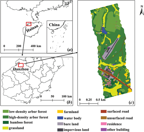
The low-density arbour forest is sparsely distributed and clearly textured young/middle age trees. The high-density arbour forest is densely distributed mature trees with no obvious texture feature. The bamboo forest occupies a small part of the study area, which is not further subdivided. The bare land refers to the area not covered by vegetation or other objects. The impervious land refers to the soil that has become sealed by cement or other material (Peroni et al. 2022). Compared to bare land, it refers specifically to land that no longer contribute to rainwater infiltration, biodiversity, plantation, or carbon storage. The surfaced road is paved with asphalt emulsion (sometimes called ‘chip-seal’) (Zhang et al. 2021). The unsurfaced road is paved with no material (Witt III et al. 2014). The residence and the other building have similar spatial information. The latter refers to the building that is not intended for human habitation, such as factories, public facilities, etc. Its materials are slightly different from those of residence.

To be further directly applied to the precise land cover classification, this paper sampled 6,000 points with category labels using random sampling tool of ArcGIS based on the ground truth value (Figure 1(c)). Those sample points were uniformly distributed. Among them, both the low-density arbour forest and the bamboo forest have 1000 sample points. The high-density arbour forest has 1200 sample points. Grassland and farmland have 600 sample points. Bare land and surfaced road both have 300 sample points. As for the other classes, each of them has 200 points. Then, we divided them to training points and testing points, in which 80% were samples for the train set, and the other 20% were samples for test set.

2.2. Data acquisition

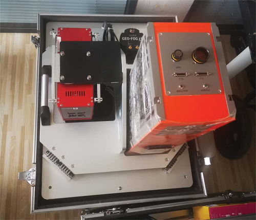
The airborne data acquisition experiment was carried out on 25 May 2020, equipped with the AisaIBIS sensor (Figure 2), flew at an altitude of 1350 m. The AisaIBIS sensor is the commercial sensor of a module of the Hyperspectral Plant imaging spectrometer (HyPlant) system (Wang et al. 2022). It can cover the red and near-infrared spectrum bands ranging from 669 to 780 nm with high signal-to-noise ratio (Siegmann et al. 2019). The flight result is shown in Figure 3.

Figure 2. The AisaIBIS sensor equipment of the airborne flight experiment.

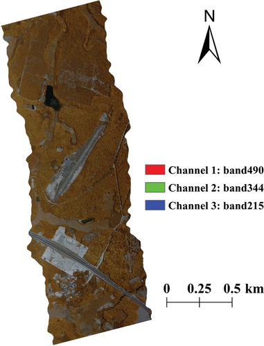
The ultra-hyperspectral data obtained by AisaIBIS sensor consists of 1004 bands with 0.11 nm spectral resolution. Its size is 1164 × 2641.The spectral coverage is 669–780 nm. The spatial resolution is 1 m. Its data size is about 5.6 GB. And its data format is BIL. In order to visually display the ground object information contained in the obtained image, false colour display was performed based on three-colour synthesis. Specifically, channel 1 corresponds to band 490, channel 2 corresponds to band 344, and channel 3 corresponds to band 215. As shown in Figure 3, false colour display result was stretched in minimum-maximum way.

Before being used in the simulation of hyperspectral data and land cover classification, the original ultra-hyperspectral data has finished preprocessing work, including clipping, radiometric correction, and atmospheric correction.

Figure 3. The data acquisition result: ultra-hyperspectral data.

To further explain the characteristics of various types of ground objects in Figure 1(c), spectral reflectance curves of 12 classes of ground objects were drawn based on the above ultra-hyperspectral data (Figure 3), as shown in Figure 4. They are calculated by averaging the spectral reflectance of the sample points of each class extracted in section 2.1. It is obvious that spectral curves of most ground objects show significant peaks and troughs between band 800 and band 900, except for water.

Figure 4. The spectral reflectance curves of ultra-hyperspectral data.

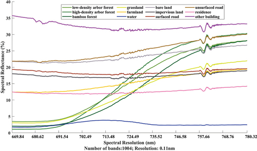
Water has the lowest spectral reflectance, at only about 2%, so it is most easily identified by spectral characteristics. In addition, the spectral reflectance of residence and other building changes similarly, showing a slight fluctuating trend. To greatly reducing the probability of mixing, it can make full use of the value difference between the two spectral curves in classification, which is about 20%. Besides, there are two categories with unique characteristics: grassland and farmland. In the beginning, their spectral reflectance differed greatly (more than 10%). Then, the spectral reflectance of the former goes up rapidly while that of latter increases steadily and slowly. And from band 600, the spectral difference suddenly became less than 2%, which would increase the chance that the two misclassify each other.

Notably, there are three groups of land cover types, each composed of the same material. Furthermore, every group of categories shows very similar spectral characteristics. It is no doubt that these factors add numerous difficulties to precise land cover classification. The first group is vegetation category: low-density arbour forest, high-density arbour forest, and bamboo forest. Their spectral reflectance curves begin with a very low spectral reflectance (less than 5%), then rapidly rise to more than 25%, and finally stay flat. The second group is impervious land and surface road. Both of their spectral reflectance curves are in the middle level (about 18%), and remained basically unchanged. The third group is bare land and unsurfaced road, which have the same spectral reflectance in band 1 (22%), and then rise slowly, although to the near-infrared band, the latter reaches 30%, but has only 3% difference with the former.

Due to the high spectral resolution of ultra-hyperspectral data, all the above classes have small differences in spectral reflectance value between each other. This subtle spectral difference is expected to contribute to the identification of such features.

3. Methodology

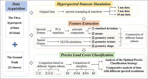
Figure 5 details the methodology used in the precise land cover classification based on ultra-hyperspectral data from AisaIBIS sensor of this paper. First, the spectral information of ultra-hyperspectral data was extracted through principal components analysis (PCA). On one hand, it eliminated redundancies. On the other hand, the key spectral information of fine ground objects was retained. At the same time, the spatial feature was extracted by grey-level co-occurrence matrix (GLCM) calculation. It is convenient to directly distinguish the features with significant spatial differences. Afterwards, a strategy for the achievement of optimal precise land cover classification of ultra-hyperspectral data was developed. It involved comparing the classification accuracy under different feature subsets and classifiers. Then, they were put into precise land cover classification to explore the optimal classification strategy. Finally, using the spectral resampling method, hyperspectral datasets with the spectral resolution of 1 nm, 5 nm, 10 nm were simulated based on ultra-hyperspectral data. The simulation datasets were classified to compare with ultra-hyperspectral data, and to verify the significance of the latter in precise classification.

Figure 5. The framework of precise classification based on ultra-hyperspectral data and hyperspectral datasets with different spectral resolutions.

3.1. The extraction of spectral features from ultra-hyperspectral data

With the increase in spectral bands and spectral resolution in ultra-hyperspectral images, the spectral information becomes more abundant, significantly benefiting image classification. Yet, studies reported that when the increase in spectral dimension reaches a critical point, the data reliability and efficiency, even the classification accuracy, would be affected (Shahshahani and Landgrebe 1994). PCA is an effective and widespread method for processing and analysing numerous spectral information in ultra-hyperspectral remote sensing research (Chen and Qian 2009; Dronova et al. 2015; Shahdoosti and Ghassemian 2016). It is an unsupervised linear technique which mainly used for embedding spectral information into a linear subspace of low dimensionality (Kambhatla and Leen 1997). The general steps involved in the PCA technique are as follows:

(a) Construct the spectral vector from $n$-dimensional spectrum information, and then calculate the data variance.

(1) $Variance=\frac{{\sum }_{i=1}^n{\left(X_i-\bar{X}\right)}^2}{n-1}$(1)

where $X_i$ is spectral reflectance value, $\bar{X}$ is the mean value of the spectral reflectance, $n$ is the number of spectral bands.

(b) Assign the direction with the largest data variance to the first principal component (i.e. X-axis).

(c) Assign the direction with the second-largest data variance to the second principal component (i.e. Y-axis), which is orthogonal to that of the first principal component.

(d) Employ this method to calculate all principal component directions.

(e) Obtain the principal component values by analysing the covariance matrix and eigenvalues of the dataset.

(f) Select $N$ principal components in accordance with the eigenvalues and eigenvectors of the covariance matrix.

(g) Rotate the original data to the new space, where the $N$ principal components are located, based on the relationship between the data and the $N$ principal components.

The essence of feature selection through PCA is to find and screen out certain principal components. The determination of the number of principal components is a key step in PCA. The following three indicators are generally used to determine which principal component should be extracted: eigenvalue, contribution rate, and scree plot test (Camargo 2022). In which the eigenvalues and contribution rate are obtained by constructing the following covariance matrix (Cov):

(2) $Cov=\frac{\sum _{i=1}^n(X_i-\bar{X})\times (Y_i-\bar{Y})}{n-1}$(2)

where $Y_i$ is the transformed principal component value, $\bar{Y}$ is the mean value of the transformed principal component.

(3) $ContributionRate=\frac{{\sum }_{i=1}^N\left(Y_i\right)}{{\sum }_{i=1}^n\left(Y_i\right)}\left(i=1,2,3,\cdots \cdots ,n\right)$(3)

In PCA, the principal components with eigenvalues of > 1 were the only ones maintained. This method is also called the Kaiser criterion. If a principal component has an eigenvalue of < 1, its contribution is considered smaller than that of a single band. Thus, it should be eliminated. Variance reflects the contribution rate of every principal component. It should be used together with the cumulative variance rate as the basis for selecting the number of principal components. The larger the rate, the richer the spectral information contained. Scree test refers to the analysis of the trend of eigenvalues. Generally, the number of principal components extracted is determined by the inflection point of the feature (Hong and Abd El-Hamid 2020).

Although the data volume is declined after reducing the feature dimension by PCA, it does not mean that there will be serious loss of spectral information. Using PCA method, the spectral feature of 1004 bands of ultra-hyperspectral data was reconstructed into 1004 principal components. They were sorted according to the amount of information. Each band would be assigned different weights when it was converted into principal components. Thus, the spectral information of all bands has a certain proportion of coverage in each principal component. Besides, in terms of the number of principal components, only principal components which cumulative contribution rate exceeds 90% can be extracted. Therefore, PCA method will retain most of the spectral features of the original ultra-hyperspectral data.

In this study, it used ENVI and MATLAB to perform PCA. In this process, the key information of the original data would be retained to the greatest extent, and the less relevant information would be eliminated. Based on the PCA results, spectral feature is obtained by further calculation, such as means and standard deviations.

3.2. The extraction of spatial features from ultra-hyperspectral data

In the study area of our research, some ground objects are difficult to distinguish by only spectral information due to spectral similarity. For example, impervious land and surfaced road have similar spectral characteristics since they used almost the same material. Yet they typically have unique geometric properties. Therefore, geometric features are introduced in this paper. They were calculated by eCognition Developer software.

Spatial features mainly include the following:

① Geometry Extent Feature.

It reflects the internal information of spatial geometry, including length $\left(l\right)$, width $\left(w\right)$, length/width, thickness, border length $\left(l_B\right)$, height, area $\left(S\right)$, volume.

② Geometry Shape Feature.

It refers to the features that reflects the relationship between geometric shapes. Such as, compactness, density, border index, shape index, roundness, etc (Basaraner and Cetinkaya 2017).

(4) $Compactness=l\times w/n$(4)

(5) $Density=n/r$(5)

(6) $ShapeIndex={\sqrt{l_B/S}}^4$(6)

where $n$ is the number of pixels of the image object, and $r$ is the approximate radius of the image object.

③ Texture Feature.

It is mainly divided into texture features based on grey-level co-occurrence matrix (GLCM) and texture features based on Gabor filters. This study selected GLCM-based texture feature in ultra-hyperspectral data classification. It mainly includes means, standard deviations, contrast, correlation, entropy, angular 2nd moment (ASM), and dissimilarity (Numbisi, Van Coillie, and De Wulf 2019).

(7) $Contrast={\sum }_{i=0}{\sum }_{j=0}p\left(i,j\right)\times {\left(i-j\right)}^2$(7)

(8) $Entropy={\sum }_{i=0}{\sum }_{j=0}p\left(i,j\right)\times lnp\left(i,j\right)$(8)

(9) $DisplayedequationASM=\sum _{i=0}\sum _{j=0}p{(i,j)}^2,$(9)

where $p\left(i,j\right)$ is a pair of pixels of GLCM, $i$ is the row number of $p\left(i,j\right)$, and $j$ is the column number of $p\left(i,j\right)$.

3.3. Exploration of optimal precise land cover classification from ultra-hyperspectral data

In ultra-hyperspectral data classification, the problem of ‘same object with different spectrum’ and ‘different object with same spectrum’ is widespread (Luo et al. 2017). It is liable to misclassify if only using spectral information in classification (Bechtel et al. 2015). Therefore, it developed the multi-feature joint object-oriented classification strategy to fully exploit the information advantage of ultra-hyperspectral data. It aims to eliminate the interference of information redundancy, and mine the spectral and spatial information that is conducive to the identification of complex objects.

We set up five sets of experiments with the help of eCognition toolbox (Michez et al. 2013).

3.3.1.

(a) Using spectral features in the classification experiment, named feature subset I, shown in Table 1.

Table 1. The description of feature subset I.

Feature subset	Description
Spectral feature	Mean (PC1–7) Standard deviation (PC1–7)

(b) Using spatial features in the classification experiment, named feature subset II, shown in Table 2.

Table 2. The description of feature subset II.

Feature subset	Description
Geometry extent feature	Area Length Width length/width Border length
Geometry shape feature	Compactness Density Shape index
Texture feature	GLCM Contrast GLCM Entropy GLCM ASM GLCM Mean GLCM Standard deviation GLCM Correlation GLCM Homogeneity GLCM Dissimilarity

(c) Using spectral and geometry extent features in the classification experiment, named feature subset III, shown in Table 3.

Table 3. The description of feature subset III.

Feature subset	Description
Spectral feature	Mean (PC1–7) Standard deviation (PC1–7)
Geometry extent feature	Area Length Width length/width Border length

(d) Using spectral, geometry shape and texture features in the classification experiment, named feature subset Ⅳ, shown in Table 4.

Table 4. The description of feature subset II.

Feature subset	Description
Spectral feature	Mean (PC1–7) Standard deviation (PC1–7)
Geometry shape feature	Compactness Density Shape index
Texture feature	GLCM Contrast GLCM Entropy GLCM ASM GLCM Mean GLCM Standard deviation GLCM Correlation GLCM Homogeneity GLCM Dissimilarity

(e) Using the combination of feature subset I and II in the classification experiment, shown in Table 5. It is named feature subset Ⅴ.

Table 5. The description of feature subset Ⅴ.

Feature subset	Description
Spectral feature	Mean (PC1–7) Standard deviation (PC1–7)
Geometry extent feature	Area Length Width length/width Border length
Geometry shape feature	Compactness Density Shape index
Texture feature	GLCM Contrast GLCM Entropy GLCM ASM GLCM Mean GLCM Standard deviation GLCM Correlation GLCM Homogeneity GLCM Dissimilarity

Through the analysis of conclusions obtained from several classification researches, this study selected the following machine learning algorithms to assess the optimal precise classification strategy of ultra-hyperspectral data: K-nearest neighbour classifier (KNN), support vector machine classifier (SVM), decision tree (DT), and random forest classifier (RF) (Wang, Zhao, and Yin 2022; Ali et al. 2022; Fazakas, Nilsson, and Olsson 1999; Mountrakis, Im, and Ogole 2011; Mutanga, Adam, and Cho 2012; Pal 2005; Pal and Mather 2005; Shataee et al. 2012; Zare Naghadehi et al. 2021). The parameters of these classifiers have been optimized by comparing the classification accuracy of different parameter combinations for each classifier. Finally, it obtained the optimal parameter settings, which shown in Table 6. They were finished with eCognition software.

Table 6. The optimal parameter setting for different classifiers.

Classifier	Parameter setting
KNN	K value: 5
SVM	Kernel function: RBF Penalty coefficient: 4 Gamma: 0.1
DT	Depth: 50 Max categories: 12 Cross validation folds: 5 Truncate pruned tree
RF	Depth: 50 Min sample count: 10 Max categories: 12 Max tree number: 100 Forest accuracy: 0.01 Active variables: 0 Termination criteria: max tree number

And the Overall Accuracy (OA) and Kappa Coefficient Accuracy (KIA) from the confusion matrix were used to evaluate the classification accuracy (Varin, Chalghaf, and Joanisse 2020). They were the average values of classification accuracy after 50 runs. The evaluation analysis was performed by MATLAB.

3.4. Contrastive classification between ultra-hyperspectral data and simulated hyperspectral datasets with different spectral resolutions

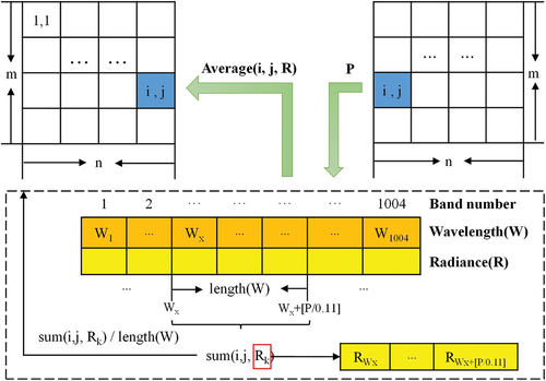
This study developed the spectral resampling method to obtain hyperspectral datasets with different spectral resolutions in MATLAB platform. The spectral resampling method mainly uses the reflectance of the image. It is to determine the band information of coarser spectrum from finer scale spectrum. So that the target data is completely consistent with the original data (the ultra-hyperspectral image), except for the different spectral resolution.

The process of spectral resampling is presented in Figure 6. First, the spectral information table of each image point $\left(i,j\right)$ of the original image was constructed, including the band number, the band wavelength $\left(W\right)$, the corresponding spectral radiance. Second, the target spectral resolution $P$ was set. Third, the spectral information table was traversed for the reflectance of a total of every $\left(P/0.11\right)$ band, with the reflectance summed $R_k$. At last, the target reflectance of $W$ was calculated by the formula sum as follows: $\left(i,j,R_k\right)/length\left(W\right)$. This operation is repeated for each image point until a new band resolution image was obtained.

Figure 6. The principle of the hyperspectral data simulation method.

After simulation experiment, we obtained various data with tens to hundreds spectral bands. The large number of spectral bands provides rich information to classification. However, the increase of bands also leads to information redundancy and high data processing complexity (Xue et al. 2021). Spectral dimensionality reduction for data with spectral bands over hundreds was conducted to reduce the interference of information redundancy and high computational complexity on classification accuracy (Luo et al. 2021).

The comparative classification between the ultra-hyperspectral data and simulated hyperspectral datasets was conducted under the same experimental conditions. Specifically, we selected the same number of samples for training and testing. The parameter settings of the above data in SVM, KNN and RF classifiers were basically consistent. They were set with reference to the results of the experiment in Section 3.3. Besides, the features used in this experiment were selected by referring to the classification results of ultra-hyperspectral data with different strategies.

4. Results

4.1. The classification results of ultra-hyperspectral data with different strategies

The classification accuracy results are shown in Table 7. Through the comparison of ultra-hyperspectral data classification with different feature subsets in the same classifier, it is found that the classification accuracy using only spectral features (74.89–83.64%) is always slightly higher than using spatial features (71.78–82.60%). Besides, the classification accuracy after combining features was superior to that of using only the spectral features and geometry features. On the basis of spectral features, no matter combined with geometric features or texture features, their contribution to classification accuracy is almost equal, which has a gap of less than 1%. Furthermore, the combination of geometric, texture, and spectral features can further play the information advantages of ultra-hyperspectral data in classification. And its improvement in classification accuracy is expected to be more significant if introducing other features rather than spectral and spatial features, such as deep learning feature (Zhou et al. 2023).

Table 7. The precise classification accuracy of ultra-hyperspectral data under different feature subsets and classifiers.

Classifier	Data	Accuracy value
		OA (overall accuracy)	KIA (Kappa coefficient accuracy)
SVM	feature subset I	74.89%	67.68%
	feature subset II	71.78%	61.77%
	feature subset III	83.62%	78.12%
	feature subset Ⅳ	82.55%	75.57%
	feature subset Ⅴ	84.20%	78.37%
KNN	feature subset I	83.21%	77.30%
	feature subset II	82.60%	74.84%
	feature subset III	85.65%	80.64%
	feature subset Ⅳ	84.77%	78.54%
	feature subset Ⅴ	86.80%	82.30%
DT	feature subset I	82.53%	76.70%
	feature subset II	78.23%	69.41%
	feature subset III	83.27%	77.09%
	feature subset Ⅳ	82.96%	76.70%
	feature subset Ⅴ	85.21%	78.66%
RF	feature subset I	83.64%	77.94%
	feature subset II	82.51%	76.54%
	feature subset III	86.65%	81.33%
	feature subset Ⅳ	86.58%	81.30%
	feature subset Ⅴ	88.44%	84.36%

Furthermore, through the comparison of ultra-hyperspectral data classification with different classifiers, it is found that different feature subsets perform better in KNN and RF classifier rather than SVM or DT classifier. And feature subset Ⅴ makes greater contribution to the improvement of classification in RF classifier. The accuracy of its classification result is also the optimal. Figure 7 shows the highest precise classification results of ultra-hyperspectral data using feature subset I to feature subset Ⅴ in different classifiers, including KNN classification result of feature II, and RF classification results of other four feature subsets.

Figure 7. The precise classification results of ultra-hyperspectral data with different feature subsets.

Through the comparison of classification results between spectral (feature 1) and spatial features (feature 2), it is found that the former is more sensitive to vegetation-related categories, which has better distinguishing effect, especially grassland, while the latter is slightly weaker. And when using only spatial feature, its advantage seems not been fully exploited. However, after combined the spectral and different parts of spatial features, the classification results improved a lot in non-vegetation categories, such as surfaced road, unsurfaced road, and impervious land. Besides, the combination of all spatial and spectral features further integrates spatial and spectral advantages, which achieves the optimal classification outcome. The classes that have improved the most are low-density arbour forest, residence, farmland, grassland, and bamboo forest. Therefore, we analysed that precise land cover classification needs a variety of features to combine to effectively play their own characteristics, so as to accurately identify ground objects.

4.2. Results of simulated hyperspectral datasets with different spectral resolutions

Through the simulation method of section 3.4, it obtained the simulated hyperspectral datasets in Figure 8 (a–c). The simulated images have the same spectral coverage (669–780 nm) and spatial resolution (1 m) as ultra-hyperspectral data. Whereas the spectral resolution and bands are various, in which 1 nm data (Figure 8(a)) has 112 bands, 5 nm data (Figure 8(b)) has 21 bands, and 10 nm data (Figure 8(c)) has 12 bands.

Figure 8. The ultra-hyperspectral data and the simulated HSI datasets with different spectral resolutions.

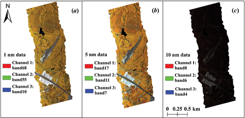
To highlight the subtle differences between simulated hyperspectral datasets and ultra-hyperspectral data obtained in Figure 3, it selected the following presentation mode: the combination of band 17 (channel 1), band 11 (channel 2), and band 7 (channel 3) of 5 nm data; the combination of band 68 (channel 1), band 55 (channel 2), and band 10 (channel 3) of 1 nm data; the combination of band 8 (channel 1), band 6 (channel 2), and band 4 (channel 3) of 10 nm data. The selected display band combination is basically close to that of ultra-hyperspectral data.

To analyse the spectral characteristics of the 12 land cover types in the simulated HSI data, we drew the spectral reflectance curves of different ground objects in the simulated HSI datasets with different spectral resolutions, using the same method as in section 2.2, which are shown in Figures 9–11. In general, all categories present similar spectral trends with those shown in Figure 4, especially impervious land and surfaced road. However, compared to ultra-hyperspectral data, they are smoother and less volatile. It would cause interference to the recognition of objects with spectral similarity, thus inhibiting the classification accuracy.

Figure 9. The spectral reflectance curves of 1nm simulated HSI dataset.

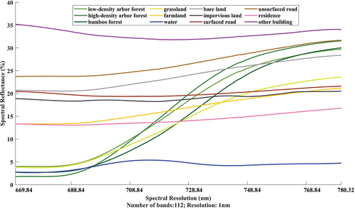
Figure 10. The spectral reflectance curve of 5nm-simulated HSI dataset.

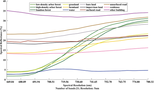
Figure 11. The spectral reflectance curves of 10nm simulated HSI dataset.

4.3. The precise classification results of ultra-hyperspectral data and simulated hyperspectral datasets

Based on ultra-hyperspectral data and simulated hyperspectral datasets, the comparative classification experiments of complex scene were carried out through SVM classifier, KNN classifier and RF classifier. It applied feature subset Ⅴ to the classification research of this section. The classification results were evaluated using the ‘Error Matrix based on TTA MASK’ provided by eCognition Developer software.

The evaluation results are shown in Table 8. In the same classifier, the classification accuracy varies greatly with the change of spectral resolution. Overall, the classification accuracy of ultra-hyperspectral data is always optimal among all classifiers. Compared with simulated hyperspectral datasets, the classification accuracy of ultra-hyperspectral data was improved in different degrees (3.58%-9.02%). Besides, by comparing the hyperspectral datasets, we found that finer spectral resolution has less contribution to the improvement of classification accuracy. For example, the classification accuracy of 5 nm data is close to that of 1 nm data in KNN classifier. Both improved by approximately 1% compared with 10 nm data. Yet, the classification accuracy of 0.11 nm data is improved by about 3%. It is similar to the result of DT classifier.

Table 8. The precise classification accuracy of the data with different spectral resolution.

Classifier	Spectral resolution	Accuracy value
		OA	KIA
SVM	10 nm	75.18%	68.36%
	5 nm	75.70%	68.99%
	1 nm	80.62%	73.23%
	0.11 nm	84.20%	78.37%
KNN	10 nm	82.06%	75.69%
	5 nm	83.03%	77.05%
	1 nm	83.14%	77.58%
	0.11 nm	86.80%	82.30%
DT	10 nm	81.37%	73.22%
	5 nm	81.84%	73.59%
	1 nm	82.68%	74.94%
	0.11 nm	85.21%	78.66%
RF	10 nm	80.30%	73.93%
	5 nm	81.52%	75.46%
	1 nm	82.47%	76.82%
	0.11 nm	88.44%	84.36%

In different classifiers, the classification accuracy of the data also has a high gap. From the value of the classification accuracy, SVM classifier obtains the lowest classification accuracy. In the comparison of classification accuracy of every simulated hyperspectral dataset, it can be found that KNN classifier is superior to DT classifier, followed by RF classifier and SVM classifier. However, for ultra-hyperspectral data, the classification using RF classifier has much higher accuracy than others.

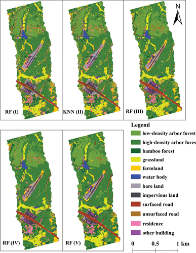
The result of Table 4 shows that the improvement of the classification strategy (feature subset Ⅴ) obtained the accuracy of 88.44%. And RF classifier is more suitable for ground object recognition of data with massive features in complex scenes.

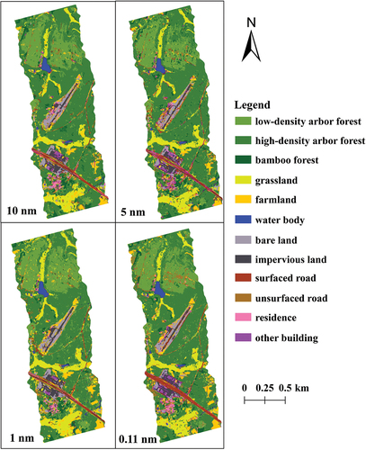
Figure 12 shows the precise classification results of the data that obtained the best classification accuracy value in different classifiers. They are: the result of 10 nm data obtained by KNN classifier (82.06%), the result of 5 nm data obtained by KNN classifier (83.03%), the result of 1 nm data obtained by KNN classifier (83.14%), and the result of 0.11 nm data obtained by RF classifier (88.44%).

In the classification results of the data with different spectral resolutions, almost all water body areas are correctly identified. The identification of their grassland areas is also basically the same. The classes with large differences in recognition were arbour forest, farmland, surfaced road, residence, and other building. In the classification results of simulated hyperspectral datasets, the farmland and other building are seriously over classified. Especially in the bottom areas, the grassland was misclassified as farmland. And the residence was misclassified as other building. Besides, the surfaced road areas were misidentified into residence and grassland.

Figure 12. The classification results of the highest classification accuracy of the data with different spectral resolution.

Compared with the simulated hyperspectral datasets, the misclassification condition of ultra-hyperspectral data has improved a great deal. In particular, the farmland that close to the grassland are more accurately identified. Besides, both wide and narrow surfaced roads have been effectively identified. And other building areas are much less mixed with residence and other objects. In the middle areas, the identification of high-density arbour forest as bamboo forest and low-density arbour forest has improved significantly.

Figure 13. The detail classification results of the highest classification accuracy of the data with different spectral resolution.

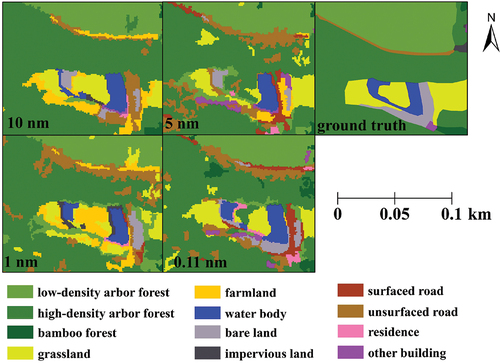
Further, we selected a classified area to enlarge and display, as shown in Figure 13. In classification results of the simulated hyperspectral datasets, only some part of areas was correctly identified. Much of the rest was misclassified as farmland, unsurfaced road, and other building. Yet they were almost completely recognized in the classification result of ultra-hyperspectral data, especially the impervious land and grassland.

5. Discussion

5.1. Analysis of the optimal precise classification strategy of ultra-hyperspectral data

This study uses ultra-hyperspectral data with higher spectral resolution. It explored the suitable data processing and classification methods of the data obtained by new AisaBIS sensor. It chose a complex scene to verify the classification potential of ultra-hyperspectral data, which has 12 classes, including five vegetation-related classes and seven non-vegetation classes. A variety of classification strategies were proposed based on different feature subsets and classifiers. The object-oriented algorithm is suitable to explore the potential about applying this sensor to classification (Tommasini, Bacciottini, and Gherardelli 2019). It takes the object as the analysis unit and is based on the image patch, which can effectively reduce the phenomenon of impulse noise in classification.

From the change degree of the classification accuracy value, the results obtained by KNN and DT classifiers changed little. It means that these two methods are not very sensitive to spectral information. Using this method for classification, the potentialities of spectral information brought by the increase of spectral resolution cannot be fully tapped. In contrast, the results obtained by SVM classifier are significantly different from each other. In general, the classification accuracy of ultra-hyperspectral data in RF classifier is the optimal. And it is also better in KNN classifier. Besides, the object-oriented algorithm makes more features involved in the classification, thus increasing the accuracy of ground object recognition.

We are of the opinion that RF classifier is more conducive to combining the rich spatial and spectral information of ultra-hyperspectral data, which greatly improved the ability of precise ground object recognition, SVM classifier comes second. While KNN and DT classifiers are less sensitive to the features of ultra-hyperspectral data using in classification experiment. As a result, the change of classification strategy makes a weak contribution to the enhancement of ground object recognition ability. Further, it is found that RF classifier is advantageous for distinguishing different vegetation-related classes. SVM classifier is very helpful for distinguishing vegetation classes from non-vegetation classes, and the identification of non-vegetation classes.

Next, we plan to explore more features of the ultra-hyperspectral data, and make full use of its information advantages. Through introducing state-of-the-art (SOTA) classification strategies, it is expected to carry out thorough research for feature extraction (Tao et al. 2022; Zhang et al. 2021). The recognition ability of ground objects in complex scenes would be further improve, such as different tree species and different crops.

5.2. Analysis of the comparison of ultra-hyperspectral data and simulated hyperspectral datasets

The data obtained by AisaIBIS sensor has a leading position for its ability of super high spectral resolution (0.11 nm), narrow bandwidth (1004 bands), and high spatial resolution (1 m). The information of ultra-hyperspectral data is quite rich in not only spectra, but also space. This study fully assessed its precise classification superiority through the simulation of hyperspectral datasets and the comparison between them. Through simulation experiment, the data with different spectral resolutions were obtained under the same research area, acquisition conditions, and spectral resolution.

The comparison between the precise land cover classification of four datasets (ultra-hyperspectral data, and simulated datasets with spectral resolution of 10 nm, 5 nm, and 1 nm) showed that the classification accuracy was improved with the increase in the spectral resolution. Using ultra-hyperspectral data, the classification result was improved more than 8%, and up to 86.65%. Thus, the improvement of the spectral resolution was sensitive to the accurate identification of objects with complex features. It is also significant for the identification of different tree species.

But the ultra-hyperspectral data of this research did not cover the near-infrared and short-wave infrared spectrum. Compared with it, the publicly available hyperspectral datasets (Folkman et al. 2001; Hong et al. 2020; Huang and Zhang 2009; Jiang et al. 2019; Liu et al. 2017) usually cover a wider range of wavelengths. However, the narrow bandwidth of ultra-hyperspectral data has unique advantages for identifying specific ground objects, since some objects are only sensitive to specific bands (Gitelson, Kaufman, and Merzlyak 1996; Wang et al. 2022).

For instance, there are grassland, impervious land, and other classes near the water body in Figure 13. Water body has specific spectral curves, so it can be easily identified. However, grassland, farmland, and arbour forest are all vegetation. So that their spectral curves are more similar. Particularly, the spectral and spatial features of grassland are closely to that of farmland.

Besides, it can only be efficiently classified by making full use of the spectral information of each band. Simultaneously, the spectral information that is redundant should be eliminated. In this study, all spectral information of 1004 bands of the ultra-hyperspectral data were recombined by feature selection of PCA from the perspectives of eigenvalue, variance rate, cumulative variance rate, and scree plot test (Camargo 2022). Although PCA method caused partial loss of the spectral information of the data, it has little effect on inhibiting classification accuracy compared with simulated hyperspectral datasets. The results showed that the selected principal components could retain the significant spectral information of the ultra-hyperspectral data, and eventually achieved the best classification accuracy.

6. Conclusion

This study obtained the precise classification strategy of ultra-hyperspectral data based on the classification experiments with different feature subsets and methods. It obtained the accuracy of 88.44% through feature subset Ⅴ combined with RF classifier. Further, this study explored the classification superiority of ultra-hyperspectral data by comparison with data of different spectral resolutions through hyperspectral datasets simulation. The classification result of ultra-hyperspectral data was superior to that of other datasets, which improved the accuracy by 5.30%-6.38% (1 nm is 83.14%, 5 nm is 83.03%, 10 nm is 82.06%). Compared with the simulated hyperspectral datasets, the ultra-hyperspectral data greatly improved the ability of ground object recognition in complex scene. It suggests that ultra-hyperspectral data has high research value in application of complex ground object identification and accurate classification of urban monitoring.

Acknowledgements

We gratefully acknowledge the Academy of Inventory and Planning, National Forestry and Grassland Administration for their help in data acquisition. We also acknowledge algorithms provided by eCognition software and MATLAB platform.

Disclosure statement

No potential conflict of interest was reported by the authors.

Additional information

Funding

This research was funded by National Natural Science Foundation of China (Grant No. 41971307), Fundamental Research Funds for the Central Universities (Grant No.2042022kf1200, 2042023kf0217), State Key Laboratory of Geo-Information Engineering (Grant No.SKLGIE2023-Z-3-1), Wuhan University Specific Fund for Major School-level Internationalization Initiatives, and LIESMARS Special Research Funding.

References

- Ali, U., T. J. Esau, A. A. Farooque, Q. U. Zaman, F. Abbas, and M. F. Bilodeau. 2022. “Limiting the Collection of Ground Truth Data for Land Use and Land Cover Maps with Machine Learning Algorithms.” ISPRS International Journal of Geo-Information 11 (6): 333. https://doi.org/10.3390/ijgi11060333.
- Basaraner, M., and S. Cetinkaya. 2017. “Performance of Shape Indices and Classification Schemes for Characterising Perceptual Shape Complexity of Building Footprints in GIS.” International Journal of Geographical Information Science 31 (10): 1952–1977. https://doi.org/10.1080/13658816.2017.1346257.
- Bechtel, B., P. J. Alexander, J. Böhner, J. Ching, O. Conrad, J. Feddema, G. Mills, L. See, and I. Stewart. 2015. “Mapping Local Climate Zones for a Worldwide Database of the Form and Function of Cities.” ISPRS International Journal of Geo-Information 4 (1): 199–219. https://doi.org/10.3390/ijgi4010199.
- Cai, Y., K. Guan, J. Peng, S. Wang, C. Seifert, B. Wardlow, and Z. Li. 2018. “A High-Performance and In-Season Classification System of Field-Level Crop Types Using Time-Series Landsat Data and a Machine Learning Approach.” Remote Sensing of Environment 210:35–47. https://doi.org/10.1016/j.rse.2018.02.045.
- Camargo, A. 2022. “PCAtest: Testing the Statistical Significance of Principal Component Analysis in R.” PeerJ 10:e12967. https://doi.org/10.7717/peerj.12967.
- Chen, Y., C. Li, P. Ghamisi, X. Jia, and Y. Gu. 2017. “Deep Fusion of Remote Sensing Data for Accurate Classification.” IEEE Geoscience and Remote Sensing Letters 14 (8): 1253–1257. https://doi.org/10.1109/LGRS.2017.2704625.
- Chen, G., and S.-E. Qian. 2009. “Denoising and Dimensionality Reduction of Hyperspectral Imagery Using Wavelet Packets, Neighbour Shrinking and Principal Component Analysis.” International Journal of Remote Sensing 30 (18): 4889–4895. https://doi.org/10.1080/01431160802653724.
- Dronova, I., P. Gong, L. Wang, and L. Zhong. 2015. “Mapping Dynamic Cover Types in a Large Seasonally Flooded Wetland Using Extended Principal Component Analysis and Object-Based Classification.” Remote Sensing of Environment 158:193–206. https://doi.org/10.1016/j.rse.2014.10.027.
- Fazakas, Z., M. Nilsson, and H. Olsson. 1999. “Regional Forest Biomass and Wood Volume Estimation Using Satellite Data and Ancillary Data.” Agricultural and Forest Meteorology 98:417–425. https://doi.org/10.1016/S0168-1923(99)00112-4.
- Folkman, M. A., J. Pearlman, L. B. Liao, and P. J. Jarecke. 2001. “EO-1/Hyperion Hyperspectral Imager Design, Development, Characterization, and Calibration.” Hyperspectral Remote Sensing of the Land and Atmosphere 4151:40–51. https://doi.org/10.1117/12.417022.
- Ghamisi, P., J. Plaza, Y. Chen, J. Li, and A. J. Plaza. 2017. “Advanced Spectral Classifiers for Hyperspectral Images: A Review.” IEEE Geoscience and Remote Sensing Magazine 5 (1): 8–32. https://doi.org/10.1109/MGRS.2016.2616418.
- Gholizadeh, A., D. Žižala, M. Saberioon, and L. Borůvka. 2018. “Soil Organic Carbon and Texture Retrieving and Mapping Using Proximal, Airborne and Sentinel-2 Spectral Imaging.” Remote Sensing of Environment 218:89–103. https://doi.org/10.1016/j.rse.2018.09.015.
- Gitelson, A. A., Y. J. Kaufman, and M. N. Merzlyak. 1996. “Use of a Green Channel in Remote Sensing of Global Vegetation from EOS-MODIS.” Remote Sensing of Environment 58 (3): 289–298. https://doi.org/10.1016/S0034-4257(96)00072-7.
- Hong, G., and H. T. Abd El-Hamid. 2020. “Hyperspectral Imaging Using Multivariate Analysis for Simulation and Prediction of Agricultural Crops in Ningxia, China.” Computers and Electronics in Agriculture 172:105355. https://doi.org/10.1016/j.compag.2020.105355.
- Hong, D., N. Yokoya, J. Chanussot, J. Xu, and X. X. Zhu. 2020. “Joint and Progressive Subspace Analysis (JPSA) with Spatial–Spectral Manifold Alignment for Semisupervised Hyperspectral Dimensionality Reduction.” IEEE Transactions on Cybernetics 51 (7): 3602–3615. https://doi.org/10.1109/TCYB.2020.3028931.
- Hornero, A., P. R. North, P. J. Zarco-Tejada, U. Rascher, M. P. Martín, M. Migliavacca, and R. Hernández-Clemente. 2021. “Assessing the Contribution of Understory Sun-Induced Chlorophyll Fluorescence Through 3-D Radiative Transfer Modelling and Field Data.” Remote Sensing of Environment 253:112195. https://doi.org/10.1016/j.rse.2020.112195.
- Huang, X., and L. Zhang. 2009. “A Comparative Study of Spatial Approaches for Urban Mapping Using Hyperspectral ROSIS Images Over Pavia City, Northern Italy.” International Journal of Remote Sensing 30 (12): 3205–3221. https://doi.org/10.1080/01431160802559046.
- Huang, H., J. Zhang, J. Zhang, J. Xu, and Q. Wu. 2020. “Low-Rank Pairwise Alignment Bilinear Network for Few-Shot Fine-Grained Image Classification.” IEEE Transactions on Multimedia 23:1666–1680. https://doi.org/10.1109/TMM.2020.3001510.
- Jia, J., J. Chen, X. Zheng, Y. Wang, S. Guo, H. Sun, C. Jiang, M. Karjalainen, K. Karila, and Z. Duan. 2021. “Tradeoffs in the Spatial and Spectral Resolution of Airborne Hyperspectral Imaging Systems: A Crop Identification Case Study.” IEEE Transactions on Geoscience and Remote Sensing 60:1–18. https://doi.org/10.1109/TGRS.2021.3096999.
- Jiang, Y., J. Wang, L. Zhang, G. Zhang, X. Li, and J. Wu. 2019. “Geometric Processing and Accuracy Verification of Zhuhai-1 Hyperspectral Satellites.” Remote Sensing 11 (9): 996. https://doi.org/10.3390/rs11090996.
- Kambhatla, N., and T. K. Leen. 1997. “Dimension Reduction by Local Principal Component Analysis.” Neural Computation 9 (7): 1493–1516. https://doi.org/10.1162/neco.1997.9.7.1493.
- Komárek, J., T. Klouček, and J. Prošek. 2018. “The Potential of Unmanned Aerial Systems: A Tool Towards Precision Classification of Hard-To-Distinguish Vegetation Types?” International Journal of Applied Earth Observation and Geoinformation 71:9–19. https://doi.org/10.1016/j.jag.2018.05.003.
- Lei, R., C. Zhang, W. Liu, L. Zhang, X. Zhang, Y. Yang, J. Huang, Z. Li, and Z. Zhou. 2021. “Hyperspectral Remote Sensing Image Classification Using Deep Convolutional Capsule Network.” IEEE Journal of Selected Topics in Applied Earth Observations & Remote Sensing 14:8297–8315. https://doi.org/10.1109/JSTARS.2021.3101511.
- Liu, J., Z. Xiao, Y. Chen, and J. Yang. 2017. “Spatial-Spectral Graph Regularized Kernel Sparse Representation for Hyperspectral Image Classification.” ISPRS International Journal of Geo-Information 6 (8): 258. https://doi.org/10.3390/ijgi6080258.
- Luo, Y.-M., Y. Ouyang, R.-C. Zhang, and H.-M. Feng. 2017. “Multi-Feature Joint Sparse Model for the Classification of Mangrove Remote Sensing Images.” ISPRS International Journal of Geo-Information 6 (6): 177. https://doi.org/10.3390/ijgi6060177.
- Luo, F., Z. Zou, J. Liu, and Z. Lin. 2021. “Dimensionality Reduction and Classification of Hyperspectral Image via Multistructure Unified Discriminative Embedding.” IEEE Transactions on Geoscience and Remote Sensing 60:1–16. https://doi.org/10.1109/TGRS.2021.3128764.
- Maxwell, A. E., T. A. Warner, and F. Fang. 2018. “Implementation of Machine-Learning Classification in Remote Sensing: An Applied Review.” International Journal of Remote Sensing 39 (9): 2784–2817. https://doi.org/10.1080/01431161.2018.1433343.
- Michez, A., H. Piégay, F. Toromanoff, D. Brogna, S. Bonnet, P. Lejeune, and H. Claessens. 2013. “LiDar Derived Ecological Integrity Indicators for Riparian Zones: Application to the Houille River in Southern Belgium/Northern France.” Ecological Indicators 34:627–640. https://doi.org/10.1016/j.ecolind.2013.06.024.
- Morales-Caselles, C., J. Viejo, E. Martí, D. González-Fernández, H. Pragnell-Raasch, J. I. González-Gordillo, E. Montero, et al. 2021. “An Inshore–Offshore Sorting System Revealed from Global Classification of Ocean Litter.” Nature Sustainability 4 (6): 484–493. https://doi.org/10.1038/s41893-021-00720-8.
- Mountrakis, G., J. Im, and C. Ogole. 2011. “Support Vector Machines in Remote Sensing: A Review.” ISPRS Journal of Photogrammetry and Remote Sensing 66 (3): 247–259. https://doi.org/10.1016/j.isprsjprs.2010.11.001.
- Mutanga, O., E. Adam, and M. A. Cho. 2012. “High Density Biomass Estimation for Wetland Vegetation Using WorldView-2 Imagery and Random Forest Regression Algorithm.” International Journal of Applied Earth Observation and Geoinformation 18:399–406. https://doi.org/10.1016/j.jag.2012.03.012.
- Numbisi, F. N., F. M. Van Coillie, and R. De Wulf. 2019. “Delineation of Cocoa Agroforests Using Multiseason Sentinel-1 SAR Images: A Low Grey Level Range Reduces Uncertainties in GLCM Texture-Based Mapping.” ISPRS International Journal of Geo-Information 8 (4): 179. https://doi.org/10.3390/ijgi8040179.
- Pal, M. 2005. “Random Forest Classifier for Remote Sensing Classification.” International Journal of Remote Sensing 26 (1): 217–222. https://doi.org/10.1080/01431160412331269698.
- Pal, M., and P. M. Mather. 2005. “Support Vector Machines for Classification in Remote Sensing.” International Journal of Remote Sensing 26 (5): 1007–1011. https://doi.org/10.1080/01431160512331314083.
- Peroni, F., S. Eugenio Pappalardo, F. Facchinelli, E. Crescini, M. Munafò, M. E. Hodgson, and M. De Marchi. 2022. “How to Map Soil Sealing, Land Take and Impervious Surfaces? A Systematic Review.” Environmental Research Letters 17 (5): 053005. https://doi.org/10.1088/1748-9326/ac6887.
- Qu, F., S. Shi, Z. Sun, W. Gong, B. Chen, L. Xu, B. Chen, and X. Tang. 2023. “Fusing Ultra-Hyperspectral and High Spatial Resolution Information for Land Cover Classification Based on AISAIBIS Sensor and Phase Camera.” IEEE Journal of Selected Topics in Applied Earth Observations & Remote Sensing 16:1601–1612. https://doi.org/10.1109/JSTARS.2023.3238467.
- Shahdoosti, H. R., and H. Ghassemian. 2016. “Combining the Spectral PCA and Spatial PCA Fusion Methods by an Optimal Filter.” Information Fusion 27:150–160. https://doi.org/10.1016/j.inffus.2015.06.006.
- Shahshahani, B. M., and D. A. Landgrebe. 1994. “The Effect of Unlabeled Samples in Reducing the Small Sample Size Problem and Mitigating the Hughes Phenomenon.” IEEE Transactions on Geoscience and Remote Sensing 32 (5): 1087–1095. https://doi.org/10.1109/36.312897.
- Shataee, S., S. Kalbi, A. Fallah, and D. Pelz. 2012. “Forest Attribute Imputation Using Machine-Learning Methods and ASTER Data: Comparison of K-NN, SVR and Random Forest Regression Algorithms.” International Journal of Remote Sensing 33 (19): 6254–6280. https://doi.org/10.1080/01431161.2012.682661.
- Shi, S., L. Xu, W. Gong, B. Chen, B. Chen, F. Qu, X. Tang, J. Sun, and J. Yang. 2022. “A Convolution Neural Network for Forest Leaf Chlorophyll and Carotenoid Estimation Using Hyperspectral Reflectance.” International Journal of Applied Earth Observation and Geoinformation 108:102719. https://doi.org/10.1016/j.jag.2022.102719.
- Siegmann, B., L. Alonso, M. Celesti, S. Cogliati, R. Colombo, A. Damm, S. Douglas, L. Guanter, J. Hanuš, and K. Kataja. 2019. “The High-Performance Airborne Imaging Spectrometer HyPlant—From Raw Images to Top-Of-Canopy Reflectance and Fluorescence Products: Introduction of an Automatized Processing Chain.” Remote Sensing 11 (23): 2760. https://doi.org/10.3390/rs11232760.
- Song, Y., J. Li, P. Gao, L. Li, T. Tian, and J. Tian. 2022. “Two-Stage Cross-Modality Transfer Learning Method for Military-Civilian SAR Ship Recognition.” IEEE Geoscience and Remote Sensing Letters 19:1–5. https://doi.org/10.1109/LGRS.2022.3162707.
- Tao, C., Y. Meng, J. Li, B. Yang, F. Hu, Y. Li, C. Cui, and W. Zhang. 2022. “MSNet: Multispectral Semantic Segmentation Network for Remote Sensing Images.” GIScience & Remote Sensing 59 (1): 1177–1198. https://doi.org/10.1080/15481603.2022.2101728.
- Tian, S., Q. Lu, and L. Wei. 2022. “Multiscale Superpixel-Based Fine Classification of Crops in the UAV-Based Hyperspectral Imagery.” Remote Sensing 14 (14): 3292. https://doi.org/10.3390/rs14143292.
- Tommasini, M., A. Bacciottini, and M. Gherardelli. 2019. “A QGIS Tool for Automatically Identifying Asbestos Roofing.” ISPRS International Journal of Geo-Information 8 (3): 131. https://doi.org/10.3390/ijgi8030131.
- Tong, X.-Y., G.-S. Xia, Q. Lu, H. Shen, S. Li, S. You, and L. Zhang. 2020. “Land-Cover Classification with High-Resolution Remote Sensing Images Using Transferable Deep Models.” Remote Sensing of Environment 237:111322. https://doi.org/10.1016/j.rse.2019.111322.
- Tu, B., C. Zhou, D. He, S. Huang, and A. Plaza. 2020. “Hyperspectral Classification with Noisy Label Detection via Superpixel-To-Pixel Weighting Distance.” IEEE Transactions on Geoscience and Remote Sensing 58 (6): 4116–4131. https://doi.org/10.1109/TGRS.2019.2961141.
- Uddin, M. P., M. A. Mamun, M. I. Afjal, and M. A. Hossain. 2021. “Information-Theoretic Feature Selection with Segmentation-Based Folded Principal Component Analysis (PCA) for Hyperspectral Image Classification.” International Journal of Remote Sensing 42 (1): 286–321. https://doi.org/10.1080/01431161.2020.1807650.
- Varin, M., B. Chalghaf, and G. Joanisse. 2020. “Object-Based Approach Using Very High Spatial Resolution 16-Band WorldView-3 and LiDar Data for Tree Species Classification in a Broadleaf Forest in Quebec, Canada.” Remote Sensing 12 (18): 3092. https://doi.org/10.3390/rs12183092.
- Wang, R., J. A. Gamon, G. Hmimina, S. Cogliati, A. I. Zygielbaum, T. J. Arkebauer, and A. Suyker. 2022. “Harmonizing Solar Induced Fluorescence Across Spatial Scales, Instruments, and Extraction Methods Using Proximal and Airborne Remote Sensing: A Multi-Scale Study in a Soybean Field.” Remote Sensing of Environment 281:113268. https://doi.org/10.1016/j.rse.2022.113268.
- Wang, Y., L. Suarez, T. Poblete, V. Gonzalez-Dugo, D. Ryu, and P. J. Zarco-Tejada. 2022. “Evaluating the Role of Solar-Induced Fluorescence (SIF) and Plant Physiological Traits for Leaf Nitrogen Assessment in Almond Using Airborne Hyperspectral Imagery.” Remote Sensing of Environment 279:113141. https://doi.org/10.1016/j.rse.2022.113141.
- Wang, Z., Z. Zhao, and C. Yin. 2022. “Fine Crop Classification Based on UAV Hyperspectral Images and Random Forest.” ISPRS International Journal of Geo-Information 11 (4): 252. https://doi.org/10.3390/ijgi11040252.
- Wei, L., K. Wang, Q. Lu, Y. Liang, H. Li, Z. Wang, R. Wang, and L. Cao. 2021. “Crops Fine Classification in Airborne Hyperspectral Imagery Based on Multi-Feature Fusion and Deep Learning.” Remote Sensing 13 (15): 2917. https://doi.org/10.3390/rs13152917.
- Wei, L., M. Yu, Y. Zhong, J. Zhao, Y. Liang, and X. Hu. 2019. “Spatial–Spectral Fusion Based on Conditional Random Fields for the Fine Classification of Crops in UAV-Borne Hyperspectral Remote Sensing Imagery.” Remote Sensing 11 (7): 780. https://doi.org/10.3390/rs11070780.
- Witt III, E. C., H. Shi, D. J. Wronkiewicz, and R. T. Pavlowsky. 2014. “Phase Partitioning and Bioaccessibility of Pb in Suspended Dust from Unsurfaced Roads in Missouri—A Potential Tool for Determining Mitigation Response.” Atmospheric Environment 88:90–98. https://doi.org/10.1016/j.atmosenv.2014.02.002.
- Xu, Y., B. Du, L. Zhang, D. Cerra, M. Pato, E. Carmona, S. Prasad, N. Yokoya, R. Hänsch, and B. Le Saux. 2019. “Advanced Multi-Sensor Optical Remote Sensing for Urban Land Use and Land Cover Classification: Outcome of the 2018 IEEE GRSS Data Fusion Contest.” IEEE Journal of Selected Topics in Applied Earth Observations and Remote Sensing 12 (6): 1709–1724. https://doi.org/10.1109/JSTARS.2019.2911113.
- Xue, F., F. Tan, Z. Ye, J. Chen, Y. Wei, and Z. Wang. 2021. “Spectral-Spatial Classification of Hyperspectral Image Using Improved Functional Principal Component Analysis.” IEEE Geoscience and Remote Sensing Letters 19:1–5. https://doi.org/10.1109/LGRS.2021.3089278.
- Xu, L., S. Shi, W. Gong, Z. Shi, F. Qu, X. Tang, B. Chen, and J. Sun. 2022. “Improving Leaf Chlorophyll Content Estimation Through Constrained PROSAIL Model from Airborne Hyperspectral and LiDar Data.” International Journal of Applied Earth Observation and Geoinformation 115:103128. https://doi.org/10.1016/j.jag.2022.103128.
- Yang, X., G. Lin, Y. Liu, F. Nie, and L. Lin. 2020. “Fast Spectral Embedded Clustering Based on Structured Graph Learning for Large-Scale Hyperspectral Image.” IEEE Geoscience & Remote Sensing Letters 19. https://doi.org/10.1109/LGRS.2020.3035677.
- Zare Naghadehi, S., M. Asadi, M. Maleki, S.-M. Tavakkoli-Sabour, J. L. Van Genderen, and S.-S. Saleh. 2021. “Prediction of Urban Area Expansion with Implementation of MLC, SAM and SVMs’ Classifiers Incorporating Artificial Neural Network Using Landsat Data.” ISPRS International Journal of Geo-Information 10 (8): 513. https://doi.org/10.3390/ijgi10080513.
- Zhang, S., T. Lu, S. Li, and W. Fu. 2021. “Superpixel-Based Brownian Descriptor for Hyperspectral Image Classification.” IEEE Transactions on Geoscience and Remote Sensing 60:1–12. https://doi.org/10.1109/TGRS.2021.3133878.
- Zhang, C., S. Wei, S. Ji, and M. Lu. 2019. “Detecting Large-Scale Urban Land Cover Changes from Very High Resolution Remote Sensing Images Using CNN-Based Classification.” ISPRS International Journal of Geo-Information 8 (4): 189. https://doi.org/10.3390/ijgi8040189.
- Zhang, S., M. Xu, J. Zhou, and S. Jia. 2022. “Unsupervised Spatial-Spectral CNN-Based Feature Learning for Hyperspectral Image Classification.” IEEE Transactions on Geoscience and Remote Sensing 60:1–17. https://doi.org/10.1109/TGRS.2022.3153673.
- Zhang, Z., J. Yang, Y. Fang, and Y. Luo. 2021. “Design and Performance of Waterborne Epoxy-SBR Asphalt Emulsion (WESE) Slurry Seal as Under-Seal Coat in Rigid Pavement.” Construction and Building Materials 270:121467. https://doi.org/10.1016/j.conbuildmat.2020.121467.
- Zhou, L., X. Ma, X. Wang, S. Hao, Y. Ye, and K. Zhao. 2023. “Shallow-To-Deep Spatial–Spectral Feature Enhancement for Hyperspectral Image Classification.” Remote Sensing 15 (1): 261. https://doi.org/10.3390/rs15010261.
- Zhu, Q., X. Guo, W. Deng, Q. Guan, Y. Zhong, L. Zhang, D. Li, and D. Li. 2022. “Land-Use/land-Cover Change Detection Based on a Siamese Global Learning Framework for High Spatial Resolution Remote Sensing Imagery.” ISPRS Journal of Photogrammetry and Remote Sensing 184:63–78. https://doi.org/10.1016/j.isprsjprs.2021.12.005.