On the extraction of the reservoirs’ waterline using polarimetric X-band SAR measurements: the case study of the San Giuliano reservoir, Italy

ABSTRACT

According to the World Bank data catalogue, $6,862$ records of reservoirs and their associated dams are present summing up a capacity of $6,197$ km³ of water. They play a crucial role in providing potable and irrigation water and, therefore, it is of paramount interest to effectively monitor such critical infrastructures. An effective approach is based on satellite remote sensing and, in particular, on the Synthetic Aperture Radar (SAR). In this paper, we critically investigate the use of polarimetric SAR measurements for reservoirs’ waterline estimation. Measurements of the novel COSMO-SkyMed Second Generation (CSG) X-band quad-polarimetric SAR related to the San Giuliano reservoir, in the South of Italy, are used to carry out an electromagnetic analysis of the different polarimetric scattering returns. Experimental results show that the cross-polarized channel, as well as the inter-channel phase, are noisy and, therefore, uninformative when used to design coherent polarimetric waterline extraction methods. From an electromagnetic viewpoint, this is due to the peculiarities of the reservoirs that call for low surface roughness and negligible wave pattern that, at once, result in a joint combination of un-tilted Bragg scattering and specular reflection. This implies that a low co-polarized backscatter and a cross-polarized signal largely below the system noise floor are to be expected. As a consequence, waterline extraction approaches that do not exploit the inter-channel phase, the so-called incoherent approaches, are shown to outperform the coherent ones.

KEYWORDS:

• Reservoir
• waterline
• SAR polarimetry

1. Introduction

Reservoirs offer an extraordinary contribution to human life and development including the storage and the management of water sources, irrigation, transportation, power generation, fishing, biodiversity preservation and recreation (Hogeboom, Knook, and Hoekstra 2018). A comprehensive mapping of reservoirs and artificial lakes worldwide was proposed in (Lehner et al. 2011), where a global reservoir and dam database was developed. They mapped 16.7 million reservoirs at global scale that result in a total water area of 305,723 km² corresponding to a potential water storage volume of about 8,069 km³ (Lehner et al. 2011). Statistics from the Food and Agricultural Organization of the United Nations reported that 1324 dammed artificial lakes have been censored in Europe (FAO 2023). Spain accounts for approximately 19% of the total number of reservoirs, while Italy is the country, together with Norway, France and United Kingdom, that hosts the largest number of dammed artificial lakes (87), i.e. about 7% of the total (FAO 2023). In Italy, most of them are derived from the damming of river networks, especially for the production of electricity. They are used both for potable and irrigation use and play an important role in flood mitigation and response to droughts. In addition, these reservoirs have often become key biodiversity spots and centres of recreational activities. Hence, preserving the integrity of reservoirs and managing their water source in a smart way have significant environmental and socio-economic impacts.

The morphological features of the reservoirs, including shape, area and perimeter, may significantly change over time due to both natural phenomena as sedimentation supply from tributary rivers, rainfall, underground water inputs/seepages and evaporation and anthropogenic activities as water supply for domestic and agricultural irrigation. All this matter makes the continuous and updated monitoring of morphological features of reservoirs a fundamental but challenging task. Those changes in water mass of reservoirs are perceived as variations of water level and surface extent depending on bathymetry and topography of the lake shores (Medina et al. 2010). Hence, the reservoir’s waterline is a key parameter (Pipitone et al. 2018; Zeng et al. 2017). The observation of reservoirs is typically performed by means of aerial, topographic and bathymetric surveys. Nonetheless, they are costly and can provide short-term information on the morphological features of lakes (Purkis and Klemas 2011). When observation of large reservoirs is due, satellite imagery represents a valuable information source that is exploited to support and complement ground and aerial surveys (Dellepiane, De Laurentiis, and Giordano 2004). Although optical satellite imagery offers a simple way to extract the waterline, the scientific community agrees in considering radar satellite measurements collected by the Synthetic Aperture Radar (SAR) the most valuable source (French et al. 2006; Gupta and Banerji 1985; Zeng et al. 2017). This is due to the fine spatial resolution, large area coverage and to the independence of solar illumination and cloud coverage. However, physical interpretation of SAR imagery can be quite cumbersome due to several factors, including the speckle that hampers image interpretation and land/water separability (Ferrentino et al. 2020,b). Before proceeding further, a brief overview of relevant studies that addressed waterline extraction from satellite SAR imagery is due. Although, in principle, most of the approaches could be applied and extended to the case of inland water bodies, here the focus is made on the studies that addressed waterline extraction and water surface estimation in case of reservoirs and lakes.

In Ding and XiaoFeng (2011), a time series of 30 HH (horizontal transmit, horizontal receive) polarized SAR scenes collected at 150 m spatial resolution by the C-band Advanced SAR (ASAR) sensor is used to monitor the Dongting lake, the second largest freshwater lake in China. The image processing technique proposed in (Liu and Jezek 2004) is applied to estimate the water surface and to evaluate temporal changes in the water area due to seasonal variability. The estimated water surface is compared with the water level measured by an in-situ hydrologic station. The estimation of the water surface of the Dongting lake and its dynamics are also studied in (Xing et al. 2018), where a time-series of 35 Sentinel-1 C-band SAR data collected at 10 m spatial resolution in dual-polarization VV+VH (vertical transmit, vertical receive + vertical transmit, horizontal receive) mode is exploited. The waterline extraction is performed by an automatic statistical-based thresholding method applied on the multi-polarization backscattering coefficients. Results are contrasted with optical satellite images, showing an overall accuracy larger than 90% with the cross-polarized backscattering channel performing best.

In (Zeng et al. 2017), the estimation of the water extent and the time variability of the water surface of the Poyang lake, the largest freshwater lake of China, are addressed by means of a time-series of 56 Sentinel-1 C-band SAR VV-polarized intensity images characterized by a spatial resolution of 20 m. An histogram-based supervised thresholding method is applied to the backscattering coefficient to extract the waterline. Results pointed out significant intra-annual variation in the water extent of the lake, but no extraction accuracy assessment is undertaken using independent data source.

The Poyang lake was analysed also in (Shen et al. 2022; Zhu et al. 2021), where C-band SAR imagery is considered. In (Zhu et al. 2021), 3 Gaofen-3 HH-polarized SAR images, collected at a spatial resolution from 5 m to 10 m are exploited. An image processing segmentation method based on multi-textural features is applied to estimate the water surface extent. Comparative analysis with respect to concurrent techniques, i.e. Markov random fields, fuzzy C-means and geometric active contour, is performed but no absolute validation is undertaken. In (Shen et al. 2022), a machine learning approach is applied on 455 ground range detected Sentinel-1 C-band SAR measurements collected in VV+VH polarizations. The water area obtained with a modified U-Net convolutional neural network is extracted with an average accuracy larger than 95%. Nevertheless, this accuracy assessment is performed on a validation dataset consisting of a subset of the whole time-series, i.e. no independent information is considered.

A waterline extraction algorithm, namely dual-threshold graph cut, is proposed in (Bao, Xiaolei, and Yao 2021), and it is tested against HH- and VH-polarized SAR images collected at both C- (Sentinel-1 and Gaofen-3) and X- (TerraSAR-X) bands over different inland water bodies as lakes, rivers and urban waters. The method, by combining multi-scale textural segmentation and Otsu thresholding algorithm, results in water area extraction accuracy larger than 99% when compared with a reference water extent manually delineated from Google Earth optical images.

In (Vickers, Malnes, and Høgda 2019), the temporal evolution of the water surface area of the Altevatn artic lake (Norway) is analysed using 485 C-band SAR measurements collected by ASAR, Sentinel-1 and Radarsat-2 sensors under different polarization channels (i.e. VV, HH and VH) at moderate-to-coarse spatial resolution (i.e. from 10 m to 75 m). The waterline extraction is performed using the unsupervised K-means clustering algorithm in combination with specific post-processing techniques. Comparison is made with in-situ water level measurements from which surface area is derived, resulting in a root mean square error of about 1%.

In (Medina et al. 2010), a time-series of 12 multi-looked HH-polarized Envisat ASAR SAR images, collected at C-band with a coarse spatial resolution of 30 m, is exploited to analyse the water area extent of the Izabal Lake (Guatemala). They adopted a state-of-the-art image processing method to extract the land/water boundary at the pixel level using different filtering approaches and automatic thresholding based on equalized histograms of backscattering values. Although results show a very high correlation, i.e. 0.9, between SAR-based estimation of the water-covered area and in-situ measurements of the water level, the average water area extracted from the SAR dataset is validated against a Geographic Information System (GIS)-based estimated area, resulting in a slight overestimation of less than 1%.

In (Li and Wang 2015), several inland water bodies located in the Spiritwood buried valley (Canada) are studied using 8 coarse resolution (30 m) Radarsat-2 quad-polarimetric SAR scenes. A combination of unsupervised K-means clustering and Otsu thresholding method is proposed that ingests a single-polarization SAR image, from which both intensity and texture information are extracted. The SAR-based water extent maps are contrasted with reference water body maps manually derived by fine spatial resolution (5 m) pansharpened multispectral SPOT-5 image. Results show an extraction accuracy characterized by a Kappa coefficient in the range 0.8–0.9. They also found that the HV (horizontal transmit, vertical receive) channel provides a land/water degree of separability larger than the co-polarized ones.

In (Behnamian et al. 2017), surface water detection is performed on different water bodies in Alberta and Ontario Canadian regions by means of 12 Radarsat-2 C-band SAR images collected in quad-polarimetric imaging mode with a spatial resolution of about 8 m. A statistically based image processing approach is considered that exploits the simple linear iterative clustering superpixel algorithm. The experimental assessment is carried out by manually tracing the water area extent obtained from corresponding WorldView-2 images. After a clean-up operation, a mismatch lower than 1% is achieved between the two water areas. Nonetheless, the HH or HV single-polarization information is only used as input of this method.

Water bodies in Ontario region, Canada, are also analysed in Zhang, Hu, and Brown (2020), where 51 quad-polarimetric Radarsat-2 C-band SAR measurements characterized by a spatial resolution of approximately 8 m are considered. An automatic thresholding method is applied to the HH-polarized intensity channel together with morphological filters to extract the water area extent. A water body map obtained by applying the Otsu thresholding algorithm on the Normalized Difference Water Index (NDWI) derived from a high-resolution multispectral SPOT image is used to assess the estimation performance. Accuracy larger than 95% is achieved. In (Ferrentino et al. 2020), the reservoir’s extent is estimated from a time-series of 29 Sentinel-1 SAR data collected in VV+VH polarization imaging mode. A processing chain is proposed that includes the development of a metric, consisting of the combination of the VV and VH scattering amplitudes, from which the water/land boundary is extracted. Experimental results suggest that the dual-polarimetric information outperforms the single-polarization intensity channels, providing an average error in estimating the water area of the reservoir – with respect to ground measurements – which is about six times lower than the best single-polarization channel (i.e. VV). In Goumehei et al. (2019), a dual-polarimetric VV+VH Sentinel-1 SAR image is considered to extract the water surface area of two reservoirs in Iran. A supervised statistical approach based on the complex Wishart Markov random field is used for the estimation. However, no accuracy assessment is performed with respect to external information sources. Some works aiming at inferring information on the water extent of inland water bodies do not use SAR measurements as the only source of information. They address this task by combining SAR data with optical images, numerical models and/or ground observations as in (Hong et al. 2015; Kreiser, Killough, and Rizvi 2018; Li and Wang 2015; Pipitone et al. 2018; Schmitt 2020). Finally, two papers, which focus specifically on reservoirs, must be mentioned (Brisco 2015; Guo et al. 2022).

The analysis of the state-of-the-art points out that, although multi-polarization SAR measurements are available, typically, single-polarization intensity channels are used to extract the waterline of water bodies. However, comparative studies clearly show the polarimetric SAR based approaches outperform the classical single-polarization ones for coastline extraction purposes, i.e, to extract the land/sea boundary. In particular, these studies clearly show the benefit of the cross-polarized channel. In this body of studies, no in-depth analysis of the noise equivalent sigma zero (NESZ) is made and no physical electromagnetic analysis is carried out.

In this study, a physically based point of view is explored to analyse the similarities and differences with an apparently identical problem regarding the SAR marine coastline extraction. By taking into account the high-quality COSMO-SkyMed (CSK) Second Generation (CSG) X-band SAR quad-polarimetric (QP) measurements acquired on the San Giuliano dammed reservoir in the South of Italy, it is shown that the very limited roughness conditions and the negligible wave pattern that characterize the reservoir make the cross-polarized channel, as well as the inter-channel phase, noisy and, therefore, uninformative. This can be physically explained according to the peculiar roughness conditions that characterize the reservoir that calls for a scattering mechanism that results from the joint combination of untilted Bragg scattering and specular reflection. This implies that a low co-polarized backscattered signal reaches the SAR antenna and the cross-polarized signal is below the NESZ. As a consequence, incoherent procedures that are based on the amplitude, i.e. no inter-channel phase is used, outperform the coherent ones which rely on the inter-channel phase.

2. COSMO-SkyMed second generation

In this section, some key information about CSG constellation is provided. Special emphasis is devoted to the newly developed polarimetric modes whose high-quality measurements are used. CSG is a constellation of four satellites equipped with X-band polarimetric SAR sensors, developed and managed by the Italian Space Agency (ASI) in operational continuity with the CSK constellation (Serva, Fiorentino, and Covello 2015). The first two CSG satellites, launched in 2019 and 2022 are already operational, while the next two are scheduled for launch in 2024 and 2025 (ASI 2021). The new imaging capabilities that characterize CSG represent a significant improvement with respect to the CSK ones in terms of spatial resolution, image quality and polarimetric acquisitions (Calabrese et al. 2015). All CSG and CSK satellites follow the same sun-synchronous orbit with a nominal height of 620 km and a period of 97 min. The three main CSG SAR imaging techniques are ScanSAR, Stripmap and Spotlight.

With reference to the Stripmap acquisition mode, three imaging modes are available that include two large swath medium resolution modes, namely Stripmap, Pingpong and QP. The Stripmap and Pingpong modes call for about 3 metre spatial resolution and 40 km × 2500 km and 30 km × 2500 km area coverage, respectively, with the former that operates at either single or dual polarization, while the latter operates in alternating burst mode using different polarizations (ASI 2021).

To the aim of this study, QP Stripmap mode is considered which is a fine resolution (i. e. 3 m) experimental mode characterized by an area coverage of 40 km × 15 km (azimuth × range). The QP imaging mode is implemented by doubling the radar pulse repetition frequency and alternating the transmitted polarization on a pulse repetition interleaving basis while receiving horizontal and vertical polarizations at the same time. The QP Stripmap imaging mode spans an incidence angle range from about 20° up to 45°, with a nominal NESZ of −25 dB (ASI 2021).

3. Theory

In this section, a primer on fundamental polarimetric concepts at the basis of all the polarimetric SAR approaches is provided enhancing some physically understood hypothesis that are often neglected in the papers devoted to coastline or waterline extraction. Hereinafter, we refer to coastline (waterline) when dealing with the extraction of the boundary between land and sea (land and waterbody of the reservoir). Finally, the metrics adopted in this analysis are described.

The electromagnetic wave backscattered off the observed scene $E^{\mathrm{s}}$ can be linked to the incident one $E^{\mathrm{i}}$ according to the Jones formalism (Guissard 1994):

(1) ${\mathit{E}}^{\mathrm{s}}=\frac{e^{-jkr}}{r}\mathbf{S}{E}^{\mathrm{i}}$(1)

where $k$ is the electromagnetic wave number, $r$ is the distance between the phase centre of the SAR antenna and the observed target and the $2\times 2$ complex $\mathbf{S}$ matrix is known as scattering matrix. It consists of complex scattering amplitudes which, assuming a linear H – V basis, can be written as $S_{ij}$ with $\{i,j\}=\{\mathrm{H},\mathrm{V}\}$. When the reciprocity condition and the backscatter alignment convention are satisfied, $S_{\mathrm{H}\mathrm{V}}=S_{\mathrm{H}\mathrm{V}}$:

(2) $\mathbf{S}=\left(\begin{array}{cc}{S}_{\mathrm{H}\mathrm{H}}& S_{\mathrm{H}\mathrm{V}}\\ S_{\mathrm{H}\mathrm{V}}& S_{\mathrm{V}\mathrm{V}}\end{array}\right)$(2)

The first-order polarimetric description provided by (1) is not able to extract reliable information from distributed and depolarizing scenes. A second-order formalism based on proper averaging of the scattering matrix elements is a mandatory choice (Cloude and Pottier 1996). In this study, the coherency matrix formalism is used that consists of defining a target scattering vector $k$ (Cloude and Pottier 1996):

(3) $k=\frac{1}{\sqrt{2}}{\left[S_{\mathrm{H}\mathrm{H}}+S_{\mathrm{V}\mathrm{V}},S_{\mathrm{H}\mathrm{H}}-S_{\mathrm{V}\mathrm{V}},2S_{\mathrm{H}\mathrm{V}}\right]}^{\mathrm{T}}$(3)

where the superscript $T$ means transpose operator. The corresponding 3 $\times$ 3 coherency matrix is defined as follows:

(4) $\mathbf{T}=⟨k{k}^{†}⟩$(4)

where $⟨\cdot ⟩$ stands for ensemble average and the superscript $†$ means complex conjugate transpose operation. The $\mathbf{T}$ matrix which, by construction, is Hermitian and semi-definite positive, includes all the polarimetric information related to the scattering scene. To extract this information, several approaches have been developed that can be roughly sorted into two classes: eigen-decomposition and model-based decomposition approaches (Cloude and Pottier 1996). The former, which stem from the Cloude and Pottier eigen-value target decomposition (Cloude and Pottier 1996), exploit the mathematical properties that characterize the coherency matrix to uniquely decompose it into deterministic matrices that play the role of elementary scattering mechanisms. Hence, the $\mathbf{T}$ matrix resulting from a generic depolarizing scene can be expressed as the incoherent sum of the elementary scattering mechanisms, each weighted by the corresponding eigenvalue (Cloude and Pottier 1996):

(5) $\mathbf{T}=\sum _{i=1}^3{\lambda }_i{u}_i{u}_i^{†}$(5)

where ${\lambda }_i$ are the real non-negative eigenvalues and ${\mathbf{T}}_i=u_i{u}_i^{†}$ is the $i-$th deterministic coherency matrix that is built from the orthogonal eigenvectors $u_i$.

The formalism provided by (5) allows defining some child parameters, e.g. the polarimetric entropy $H$ and the mean scattering angle $\bar{\alpha }$, which can be effectively used to describe the polarimetric properties of the observed scene.

The randomness of the polarimetric scattering process is measured by the polarimetric entropy:

(6) $0\le H=-\sum _{i=1}^3{p}_i{log}_3{p}_i\le 1$(6)

where

(7) $p_i=\frac{{\lambda }_i}{{\sum }_{i=1}^3{\lambda }_i},{\lambda }_1\ge {\lambda }_2\ge {\lambda }_3\ge 0$(7)

are known as pseudo-probabilities. A polarimetric scattering resulting from one well-defined mechanism calls for $H$ = 0; while a mixture of scattering mechanisms calling for the same occurrence probability results in $H$ = 1. The mean scattering angle can be defined from the eigenvalue decomposition of the coherency matrix as follows:

(8) $0^{\circ }\le \bar{\alpha }=\sum _{i=1}^3{p}_i{\alpha }_i\le {90}^{\circ }$(8)

where

(9) ${\alpha }_i=cos{\left(\left|u_i(1)\right|\right)}^{-1}$(9)

In (9), ${\alpha }_i$ represents the phase related to the $i$-th elementary scattering mechanism associated to the corresponding $i$-th eigenvector, while the mean scattering angle represents the average phase related to the scattering mechanism. $\bar{\alpha }$ values close to 0° (90°) correspond to single- (double-) reflection surface scattering mechanism, while $\bar{\alpha }$ values close to 45° are associated to multiple-reflections that occur in case of volume scattering.

Model-based approaches, pioneered by the three-component Freeman-Durden decomposition (Freeman and Durden 1998), are to model the coherency (or covariance) matrix as the weighted sum of known scattering mechanisms, e.g. surface scattering, double-bounce scattering and volumetric scattering (Freeman and Durden 1998).

Focusing on reservoir waterline extraction, the approaches proposed in literature mimic the polarimetric rationale developed to extract the coastline associated to the land/sea boundary. This means that the key scattering assumption relies on the fact that the water and the land areas call for distinctive scattering behaviours. Under such a rationale, the water area, under moderate wind conditions and intermediate incidence angles, is expected to call for Bragg or tilted-Bragg scattering. The land area is expected, in general, to call for a more heterogeneous scattering behaviour that may result in the combination of surface, double-bounce and volumetric scattering. This behaviour results in completely different $H/\bar{\alpha }$ parameters over land and sea; with land calling – in general – for values larger than the sea ones. In addition, the different dielectric properties of land and sea areas are typically such that the backscattering from land is larger than the water one for a pixel roughness condition. As a consequence, child parameters are meant to distinguish land and water according to the different dielectric and roughness properties. The diagonal elements of the coherency matrix can be exploited to extract information about the dielectric properties of the observed scene (Hajnsek, Pottier, and Cloude 2003):

(10) $\epsilon =\frac{T_{22}+T_{33}}{T_{11}}$(10)

or its roughness properties by evaluating the coherence between the left-left and right-right circular polarizations (Hajnsek, Pottier, and Cloude 2003):

(11) ${\mathrm{\Gamma }}_{\mathrm{L}\mathrm{L}\mathrm{R}\mathrm{R}}=\frac{T_{22}-T_{33}}{T_{22}+T_{33}}$(11)

Both (10) and (11) are expected to emphasize land/sea separation owing to the different dielectric (10) and roughness (11) properties of the two scenarios. In a similar fashion, the model-based decomposition parameters can be used to distinguish land from water using the power of the surface and volumetric components $P_{\mathrm{S}}$ and $P_{\mathrm{V}}$, respectively (Ferrentino, Nunziata, and Migliaccio 2017; van Zyl, Papas, and Elachi 1987). The above-mentioned theoretical rationale and the polarimetric parameters have been successfully tested over coastline associated to the land/sea boundary.

Inland waters may differ substantially from sea both in terms of dielectric constant and roughness. In particular, roughness is generally expected to be significantly smaller than the sea case mimicking a partially developed sea case under low wind conditions. This makes reservoirs’ water area similar to the low backscatter area that appears on sea surface under low wind conditions (Corcione et al. 2021; Skrunes, Brekke, and Doulgeris 2015). In addition, a negligible wave structure is expected. From a polarimetric viewpoint, those differences affect noticeably both the intensity of the backscatter signal and the phase relationship among polarimetric channels, i.e. the inter-channel phase (Buono et al. 2019). In fact, the smoother reservoir surface is expected to call for a scattering mechanism that is the weighted combination (according to the SAR incidence angle) of specular reflection and un-tilted Bragg scattering (Montuori et al. 2016; Nunziata, Sobieski, and Migliaccio 2009). This means that: a) a co-polarized backscattered signal lower than the correspondent sea one is to be expected; b) theoretically no cross-polarized signal is to be expected. This latter condition, in practical cases, results in a cross-polarized backscatter below the NESZ.

4. Experiments

In this study, we discuss the extraction of the reservoirs’ waterline by investigating the QP approaches formerly described. QP coherent parameters are derived from SAR measurements using a 9 × 9 sliding window to reduce speckle noise, ensure reliable estimation and preserve spatial resolution. The extraction procedure is also carried out using the normalized radar cross section (NRCS), i. e. incoherent metrics, associated to the three polarimetric channels, namely ${\sigma }_{\mathrm{V}\mathrm{V}}^0$, ${\sigma }_{\mathrm{H}\mathrm{H}}^0$ and ${\sigma }_{\mathrm{H}\mathrm{V}}^0$. In addition, a dual-polarimetric incoherent metric that consists of evaluating the inter-channel amplitude correlation:

(12) $\mathrm{R}{\mathrm{S}}_{\mathrm{H}}=⟨\left|S_{\mathrm{H}\mathrm{H}}\right|\cdot \left|S_{\mathrm{H}\mathrm{V}}\right|⟩$(12)

is also used since it has been successfully used in (Nunziata et al. 2016; Di Luccio et al. 2019; Ferrentino et al. 2020, 2020b; Zahriban et al. 2022) to extract the coastline from C- and X-band SAR imagery collected under different coastal morphology including sandy beaches, wetlands and ice tongues. Note that also the incoherent multi-polarization metrics are evaluated by multi-looking SAR measurements using a 9 × 9 sliding window.

4.1. Study area and dataset

The San Giuliano Reservoir is a dammed artificial water basin that belongs to a protected natural area in the Basilicata region, south of Italy (40°36’50”N, 16°30’06”E), few kilometres south of the city of Matera, see Figure 1.

Figure 1. Reference map of Italy and Basilicata (in blue). The marker shows the San Giuliano reservoir.

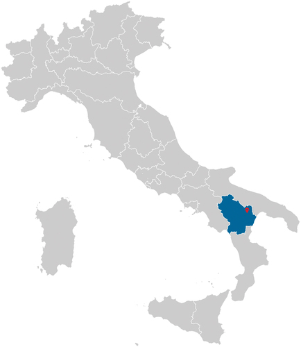
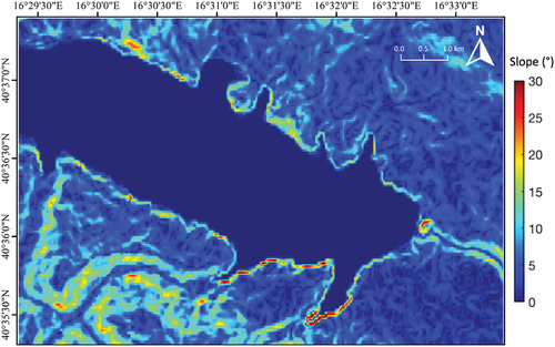
On average, it is characterized by an about 8.0−9.3 km² surface and a 100 m − 150 m depth, calling for a storage water capacity of about 10⁸ m³. The reservoir is located in a hilly area that extends between 200 m and 450 m above sea level, with steep slopes up to about 30° (Lo Curzio, Russo, and Caporaso 2013). To provide a clearer view of the slopes characterizing the area that surrounds the reservoir, the latter are extracted from the 30 m Shuttle Radar Topograhy Mission (SRTM) Digital Elevation Model (DEM), see Figure 2. Most of the study area, i.e. about 86%, calls for quite gently slopes ($<{10}^{\circ }$), while only few areas are characterized by steep slopes ($>{20}^{\circ }$). Nevertheless, focusing on the San Giuliano reservoir profile, it can be noted that its coastal morphology shows significantly large variability, from almost flat (see the northwestern coast and the bay located at about 40°37’0”N,16°31’0”E) up to very steep (see most of the northern coast and the south-southeastern coastal area, including the dam located at about 40°36’0”N,16°32’45”E) slopes. The reservoir was built in the sixties over the Bradano river for irrigation purposes and, nowadays, it provides water to a surrounding area of more than 200 km². In addition, the reservoir was elected by the European Commission as a Site of Community Importance and a Special Protection Zone due to its biodiversity heritage.

Figure 2. Slope map derived from the 30 m SRTM DEM.

The data set consists of SAR and optical images. The SAR scene was acquired by CSG in an ascending orbit on 23 August , 16:45 Universal Time Coordinated (UTC) and it includes a large part of the reservoir, i.e. about 72% of the water surface. The scene is acquired in QP imaging mode and covers an area of 40 km × 15 km with a very fine spatial resolution of 2.2 m × 1.3 m and an incidence angle equal to 38.5°. At the time of the CSG SAR acquisition, a water level of about 96 m above sea level and a water storage of about $32\cdot {10}^6$ m³ is reported by the Consortium of San Giuliano Dam. An optical image was acquired by the European Space Agency (ESA) Sentinel-2 multi-spectral sensor on 22 August , 9:40 UTC, under clear sky conditions. Sentinel-2 images collected in the visible frequency bands call for a spatial resolution of 10 m. An excerpt of the CSG HH-polarized SAR intensity image superimposed onto the corresponding excerpt of the Sentinel-2 true-colour one is depicted in Figure 3.

Figure 3. An excerpt of the CSG HH-polarized SAR scene collected on 23 August 2021, 16:45 UTC superimposed onto an excerpt of the ESA Sentinel-2 true-colour image collected on 22 August 2021, 9:40 UTC.

4.2. Experimental results

In this section, first, the waterline is extracted from the CSG SAR scene using the multi-polarization metrics and the extraction performance is inter-compared with the waterline extracted from the optical image.

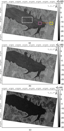
An excerpt of the CSG SAR scene that includes the reservoir and its surrounding is shown in Figure 4, where the VV-, HH- and HV-polarized NRCS graytones images, in decibel (dB) scale, are shown in panels (a), (b) and (c), respectively.

Figure 4. Excerpt of the VV- (a), HH- (b) and HV- (c) polarized NRCS graytones images (dB scale is used). The CSG SAR scene includes the reservoir and its surrounding. The transect and the ROIs used for quantitative analysis are depicted in (a) as an orange line and magenta, yellow and dashed white boxes, respectively.

First, QP coherent metrics are evaluated on the area of interest. The analysis is carried out using the child parameters derived by the eigen-decomposition of the coherency matrix. It is worth noting that those parameters include both backscattering intensity and phase information from all the three polarimetric measurement channels.

The $H$ and $\bar{\alpha }$ images are shown in Figure 5(a,b), respectively; while $\epsilon$ and ${\mathrm{\Gamma }}_{\mathrm{L}\mathrm{L}\mathrm{R}\mathrm{R}}$ are depicted in Figure 6(a,b), respectively. By visually inspecting both images, it is hard to clearly identify the water-land boundary. This implies that neither $H$ nor $\bar{\alpha }$ images result in enough land/water contrast to be used for waterline extraction purposes. In fact, when dealing with polarimetric entropy, $H$ values span from about 0.4 to 1 over both the reservoir and the surrounding coastal area. The latter calls for larger values along the coast with the exception of the north-western part, mostly depending on the scattering randomness level of the environment (sandy beaches, vegetation, etc.). When dealing with mean scattering angle, $\bar{\alpha }$ values fall in the range of approximately 35° − 55° over both water and land, with the largest values observed along the southern and eastern part of the reservoir.

Figure 5. QP analysis. False colour images related to: (a) $H$, see (6) and (b) $\bar{\alpha }$, see (8).

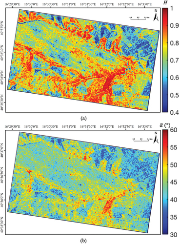
Figure 6. QP analysis. False colour images related to: (a) $\epsilon$, see (10) and (b) ${\gamma }_{\mathrm{L}\mathrm{L}\mathrm{R}\mathrm{R}}$, see (11).

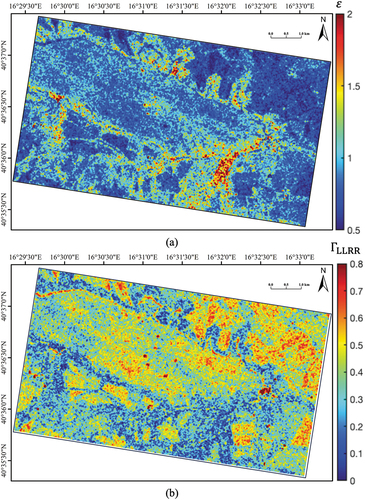
The analysis of the coherent QP features shows that, even though a quasi-deterministic surface scattering is expected over the small-roughness water surface, a large part of the pixels call for high entropy and mean scattering angle values which are non-representative of such scattering process. A completely similar behaviour applies for $\epsilon$ and ${\mathrm{\Gamma }}_{\mathrm{L}\mathrm{L}\mathrm{R}\mathrm{R}}$ (see Figure 6) that are not able to well separate land from water.

Such odd results are not due to the specific QP features adopted but to a subtle physical difference with respect to the coastline extraction case. In order to provide a physical understanding of these results, let us first re-analyse the images of Figure 4. The reservoir is characterized by a backscattered signal lower than its surrounding at all the polarizations. The low backscatter signal within the waterbody is a typical characteristic of reservoirs that, unlike the sea, in general call for limited roughness and a negligible wave pattern and can be considered as the analogue of the low backscatter area resulting from sea surface under low wind conditions.

When using polarimetric coherent information under such low roughness conditions, a data quality analysis is due. This latter consists of contrasting the backscatter level of polarimetric SAR channels with the system NESZ. Accordingly, Figure 7 shows the results of the noise analysis carried out generating a composite false colour image where red, green and blue colours refer to VV-, HH- and HV-polarized NRCS pixels, respectively, that satisfy the following condition:

(13) ${\sigma }_{ij}^0(\mathrm{d}\mathrm{B})\le (\mathrm{N}\mathrm{E}\mathrm{S}\mathrm{Z}{)}_{\mathrm{d}\mathrm{B}}+3\mathrm{d}\mathrm{B}$(13)

Figure 7. Data quality analysis. False colour composite noise map where red, green and blue colours are used to code pixels which are noisy in VV, HH and HV channel, respectively, according to the considered noise threshold.

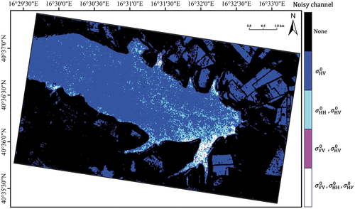
This condition is more restrictive than NESZ but it is generally adopted in both land and sea polarimetric SAR studies (Ivonin et al. 2016; Minchew, Jones, and Holt 2012). In Figure 7, red, green and blue areas represent noisy pixels in VV, HH and HV polarization channels, respectively; while black and white regions refer to noise-free pixels and pixels corrupted by noise in all polarization channels, respectively. The image shows that the cross-polarized channel is noisy everywhere over the reservoir making the coherent polarimetric analysis, i.e. the analysis that jointly exploits amplitude and inter-channel phase information, unfeasible. In addition, most of the pixels belonging to the eastern/south-eastern part of the reservoir are such that the three backscattering channels are corrupted by noise. Hence, the experimental result shown in Figure 7 suggests that the waterline extraction based on coherent features is severely hampered by noise.

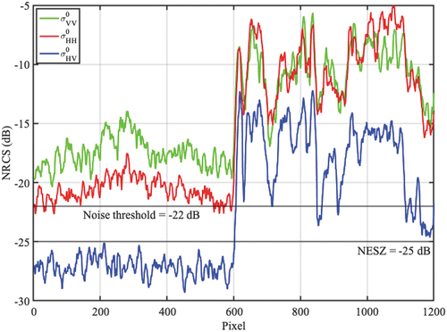
All this matter suggests investigating the behaviour of incoherent metrics over both land and sea. The analysis of the three polarimetric channels (see Figure 4) shows that the VV-polarized image (Figure 4(a)) results in the largest backscatter over both land and reservoir while the lowest backscatter results from the cross-polarized channel (Figure 4 (c)). This behaviour is quantitatively discussed in Figure 8, where the NRCS associated to the three channels, evaluated along with a randomly selected 1200 pixels-long transect crossing land and water areas and depicted as an orange line in Figure 4(a), is shown together with the NESZ and the noise threshold (13). Over the water-covered area (up to pixel number 600), the largest NRCS is achieved by the VV-polarized channel (see the green plot) which is well-above both the selected noise threshold and the NESZ. The HH-polarized channel (see the red curve) is almost everywhere above the noise threshold and everywhere above the NESZ. The lowest NRCS results from the HV-polarized channel (see the blue plot) that is always below both the NESZ and the noise threshold. This means that it has to be expected that the information extraction process based on coherent polarimetric information is significantly corrupted by noise when the cross-polarized channel is included. Along the transect, the mean VV- and HH-polarized NRCS values are around −18 dB and −20 dB, while the average HV-polarized NRCS is about −27 dB. Over the land-covered area (from pixel number 601 up to pixel number 1200), a backscatter larger than the water-covered one applies for all the channels. The two co-polarized channels are always well-above the NESZ resulting in almost overlapped NRCS values, while a lower contribution arises from the cross-polarized channel that, however, is almost everywhere above the noise threshold and everywhere above the NESZ. The average VV- and HH-polarized NRCS values are around −10 dB, while the mean HV-polarized NRCS value is around −18 dB. This means that, over land, it has to be expected a successful information extraction process using coherent polarimetric descriptors since the polarimetric channels are mostly well-above the system noise.

Figure 8. NRCS values evaluated along with the orange transect shown in Figure 4 (a) for VV (green line), HH (red line) and HV (blue line) channels. Note that the CSG NESZ and the noise threshold adopted for the data quality analysis, see (13), are also annotated as black lines for reference purposes.

To further discuss the land/water separability achieved using incoherent metrics, the empirical probability density function (pdf) is evaluated over two equal-size regions of interest (ROI), each consisting of 10,000 samples, randomly excerpted over water and land areas, see magenta and yellow box in Figure 4(a), respectively. Results are shown in Figure 9, where continuous and dashed lines refer to water and land ROI, respectively; while green, red and blue colours stand for VV-, HH- and HV-polarized channels, respectively. As far as for Figure 8, both the NESZ and the noise threshold are also annotated. By visually inspecting the plot, a remarkable land/water separability is achieved by all the metrics with the largest separation is achieved by the HH-polarized NRCS followed by the VV-polarized one.

Figure 9. Empirical pdfs evaluated within the water (continuous plots) and land (dashed plots) ROIs for the VV HH and HV channel, see green, red and blue lines, respectively. Note that the CSG NESZ and the noise threshold adopted for the data quality analysis, see (13), are also annotated as black lines for reference purposes.

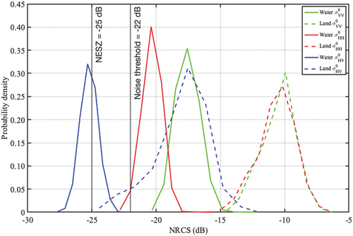
It can be noted that, as far as for the previous analysis, the co-polarized NRCSs are always above the NESZ; while the cross-polarized NRCS is largely below the NESZ and largely below the noise threshold. This means that the cross-polarized channel is noisy over the reservoir. When dealing with the land ROI, all the polarimetric channels lie above the NESZ; while only few pixels related to the HV-polarized channel are below the noise threshold. It is important to underline that such a low level of signal over reservoirs is not related to the poor quality of the CSG X-band SAR system but on the particular backscattering mechanism over the reservoir water. To discuss quantitatively the land/water backscattering separability, the Bhattacharyya distance $B$ is evaluated for each polarimetric channel, whose results are listed in Table 1 (Morio et al. 2009; Nunziata, Buono, and Migliaccio 2018):

(14) $B=-ln(\sum _{x\in X}\sqrt{(l(x)w(x)})$(14)

Table 1. Bhattacharyya distance estimated among the water and land ROI pdfs for the VV-, HH- and HV-polarized NRCSs.

Polarimetric channel	VV	HH	HV
B	6.70	7.76	5.48

where $l$ and $w$ represent the value assumed by the NRCS in the pixel under test $x$ belonging to the land and water ROIs, respectively, and $X$ = 10000 is the number of ROI samples. All the polarimetric channels provide a satisfactory land/water separability, i.e. $B$ values from about 5.5 to approximately 8 are measured. Results listed in Table 1 show that the HH- (HV-) polarized NRCSs provides the largest (lowest) land/water separability as it was found by visually inspecting Figure 9. This analysis also suggests that, although the cross-polarized backscattering channel is below the NESZ, it provides enough land/water separability to be used to extract the waterline. This agrees with literature studies that found the cross-polarized channel is the most effective one for waterline extraction purposes (Behnamian et al. 2017; Li and Wang 2015; Xing et al. 2018). According to the obtained results, hereinafter we focus on incoherent single- and dual-polarimetric approaches that have been shown to be the preferred choice to extract reservoir waterline.

To generate a binary image where land and water are clearly distinguishable, a constant false alarm rate (CFAR) detector is designed and applied to the incoherent features. This means that the statistical distribution of the water must be analysed. The empirical distribution of ${\sigma }_{\mathrm{V}\mathrm{V}}^0$, ${\sigma }_{\mathrm{H}\mathrm{H}}^0$ and ${\sigma }_{\mathrm{H}\mathrm{V}}^0$ is analysed over a randomly selected water ROI consisting of 35,000 samples (see the white dashed box in Figure 4(a)) using the Kolmogorov–Smirnov test and is found to be well-approximated (with a $5\mathrm{\%}$ significance level) by a Lognormal distribution (Berger and Zhou 2014; Davis et al. 1978). Accordingly, the relationship between the false alarm probability $P_{\mathrm{f}\mathrm{a}}$ and the CFAR global threshold $t$ is set according to a Lognormal model (Weinberg and Tran 2018):

(15) $P_{\mathrm{f}\mathrm{a}}={\int }_t^{\mathrm{\infty }}\frac{\alpha {\beta }^{\alpha }\mu r^{\mu -1}}{{\left(\beta +r^{\mu }\right)}^{\alpha +1}}dr,r>0$(15)

where $r$ is the NRCS value of the pixel under test, $\alpha$ and $\mu$ are the non-negative shape parameters, while $\beta$ is the non-negative scale parameter. On this basis, according to (15) the CFAR threshold can be obtained as:

(16) $t={\left(\beta \left[P_{\mathrm{f}\mathrm{a}}^{-\frac{1}{\alpha }}-1\right]\right)}^{\frac{1}{\mu }}$(16)

The waterline extracted from co- and cross-polarized channels using a $P_{\mathrm{f}\mathrm{a}}$ equal to ${10}^{-6}$ and ${10}^{-8}$, respectively, is depicted in Figure 10, where the waterlines extracted using the VV, HH and HV channels are superimposed – as a green, red and blue lines, respectively – onto the corresponding NRCS graytones image (in dB scale). Note that the selected $P_{\mathrm{f}\mathrm{a}}$ values refer to the best extraction result for each channel.

Figure 10. Waterlines extracted from VV (a), HH (b) and HV (c) channels superimposed as a green, red and blue lines, respectively, onto the corresponding NRCS graytones images.

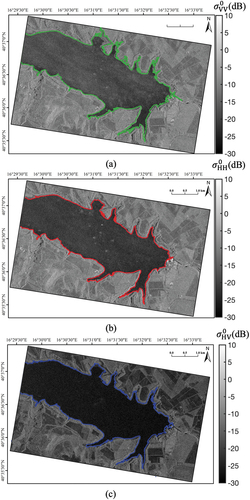
By visually contrasting the extracted waterlines with the background NRCS images, one can note that there is a generally good agreement. The HH (panel b) and HV (panel c) channels provide the best visual matching; while the waterline extracted using the VV (panel a) channel appears to call for more false alarms. This finding agrees with the results shown in Table 1.

To verify the accuracy of the extracted waterline against independent remotely sensed measurements, the three waterlines are superimposed onto the true-colour Sentinel-2 optical image, see Figure 11 where the VV, HH and HV extracted waterlines are depicted using green, red and blue lines, respectively. Results shown in Figure 11 confirm that the waterline extracted by the VV-polarized NRCS often deviates (mainly landwards) remarkably from the reservoir profile visually inspected from the optical image. To better analyse the behaviour of the extracted waterlines, selected ROIs are considered, see the four black boxes in Figure 11 that are labelled as ‘ROI 1’ up to ‘ROI 4’, whose enlarged versions are depicted in Figure 12(a-d) for ‘ROI 1’ up to ‘ROI 4’, respectively.

Figure 11. Waterlines extracted from VV- (green), HH- (red) and the HV-polarized (blue) NRCS superimposed onto the Sentinel-2 true-colour optical image. Note that black boxes are annotated that refer to the 4 ROIs selected for a detailed analysis.

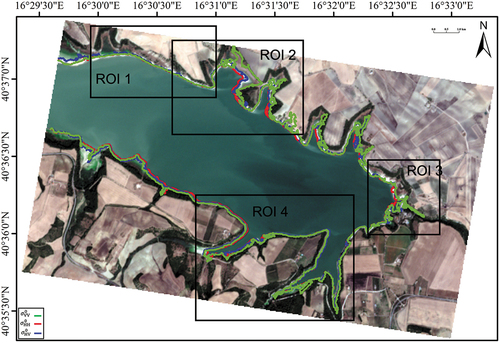
Figure 12. Enlarged version of the ROIs highlighted in Figure 11, where the extracted waterlines are superimposed as green (VV), red (HH) and blue (HV) lines. Panels (a) - (d) refer to ‘ROI 1’ - ‘ROI 4’, respectively.

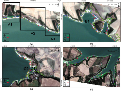
The ‘ROI 1’, see Figure 12(a), calls for a very heterogeneous coastal region that includes two bays (see the annotated ‘A1’ box) that are almost completely populated by poplars, willows and tamarisk trees. Next to the bays, an almost non-vegetated area calling for steep slope is in place (see the annotated ‘A2’ box); while the eastern part of the coast (see the annotated ‘A3’ box) is a mainly gentle slope vegetated area. The three extracted waterlines result in a good agreement with the visually inspected profile and none of them extract the waterline inside the bays that are almost completely filled with sea plants.

The ‘ROI 2’, see Figure 12(b), again calls for a coastal region that alternates almost vegetation-free steep slope areas (western part), a sandy beach (the central part of the first bay annotated as ‘B1’) and fully vegetated regions (the east side of the second bay annotated as ‘B2’). In this case, remarkable differences apply in the waterlines extracted using the three polarimetric channels. By visually contrasting the extracted waterlines with the profile of the optical image, it can be noted that along the western part up to the bay ‘B1’, the three waterlines are almost completely overlapped. In the bay ‘B1’, the HH and HV profiles provide the best agreement with the optical one; while the VV profile results in landward false edges related to vegetation. The same applies in the ‘B2’ bay and in the eastern side of the ROI, where the VV profile results in false edges coming for a bare soil area next to the steep coast.

The ‘ROI 3’, see Figure 12(c), includes also the dam of the Bradano river (see ‘C1’) which is the area where the extracted waterlines exhibit the largest deviation from one another, with the VV one resulting in a profile that goes towards the river. It is worth noting that all the extracted profiles identify the pier (see ‘C2’) that can be hardly be observed in the coarser resolution optical background image. Next to the pier, a false edge is detected in the HH profile that is likely related to a ghost image (resulting from ambiguities) into the waterbody.

The ‘ROI 4’, see Figure 12(d), calls for an almost entirely vegetated coast whose waterline is well followed by the three extracted profiles with a slightly worse agreement achieved by the VV channel.

In conclusion, by jointly analysing experimental results shown in Figures 11 and 12, the waterlines extracted using the HH and HV backscattering channels fit best the reservoir waterline visually inspected from the optical image. To further inter-compare SAR-derived waterlines with the optical information, the Sentinel-2 optical image is processed to obtain the 10 m resolution Normalized Difference Vegetation Index (NDVI) (Lastovicka et al. 2020):

(17) $-1\le \mathrm{N}\mathrm{D}\mathrm{V}\mathrm{I}=\frac{B_8-B_4}{B_8+B_4}\le 1$(17)

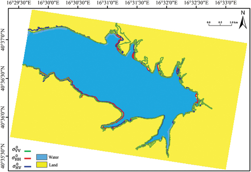
where $B_4$ and $B_8$ refer to the NIR (near-infrared) and red Sentinel-2 spectral bands. The NDVI is sensitive to the presence of green vegetation at different density scales. Non-positive NDVI values are associated to non-vegetation targets as water bodies and built-up areas, while positive NDVI values characterize vegetation (the closer to 1 is the NDVI value, the denser the vegetation is). To the aim of this study, the NDVI image is manually clustered in water and non-water, i.e. land, classes (see cyan and yellow areas in Figure 13, respectively). Hence, in Figure 13, the waterlines extracted from the multi-polarization NRCSs (green, red and blue colour refer to VV-, HH- and HV-polarized NRCS) are superimposed onto the binary-clustered NDVI image. Experimental results confirm that the waterlines extracted from HH and HV channels fit best the NDVI-based profile, while the VV channel results in several landward false alarms (see north/north-eastern part of the reservoir).

Figure 13. Waterline extracted using VV- (green line), HH- (red line) and HV-polarized (blue line) NRCS superimposed onto the NDVI clustered image where cyan and yellow stand for water and land areas, respectively.

To discuss the ability of dual-polarimetric incoherent information in improving waterline extraction, the reservoir profile was extracted using the $\mathrm{R}{\mathrm{S}}_{\mathrm{H}}$ metric (12). The same waterline extraction methodology used to process the multi-polarization NRCSs is adopted since $\mathrm{R}{\mathrm{S}}_{\mathrm{H}}$, when evaluated over the water area, also follows a Lognormal pdf model. The waterline extracted from $\mathrm{R}{\mathrm{S}}_{\mathrm{H}}$ is contrasted with the one estimated from ${\sigma }_{\mathrm{H}\mathrm{H}}^0$ since it was shown to be the single-polarization intensity channel that provides the best accuracy. Accordingly, Figure 14 shows the extracted profiles related to $\mathrm{R}{\mathrm{S}}_{\mathrm{H}}$ and ${\sigma }_{\mathrm{H}\mathrm{H}}^0$ overlaid as purple and red lines, respectively, onto the binary-clustered NDVI image. The two waterlines are almost everywhere perfectly overlapped showing that there is no significant improvement associated to the dual-polarimetric incoherent information.

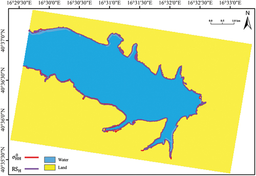
Figure 14. Waterlines extracted using $\mathrm{R}{\mathrm{S}}_{\mathrm{H}}$ (purple line) and ${\sigma }_{\mathrm{H}\mathrm{H}}^0$ (red line) superimposed onto the NDVI clustered image where cyan and yellow stand for water and land areas, respectively.

5. Discussion

The extraction of the waterline related to reservoirs has been addressed in the literature using both C- and X-band multi-polarization SAR measurements using approaches that mimic the SAR coastline extraction, i.e. the extraction of the land/sea boundary.

The analysis here performed can be summarized as follows:

1. QP coherent metrics, which have been successfully used in the literature, are applied to emphasize land/water separation, i.e., a key step to extract the waterline.

2. Results show that the cross-polarized channel and the inter-channel phase are noisy over the water-body area.

3. This behaviour can be physically explained due to the peculiarity of the reservoirs that call for a limited roughness and a negligible wave pattern. This means that the interaction between the electromagnetic wave and the water is mainly ruled by the joint combination of untilted Bragg and specular scattering. The latter result in a theoretically zero cross-polarized backscatter and - according to the roughness level and the incidence angle - a low co-polarized backscatter. This means that it is worth expecting to measure a low co-polarized NRCS and a cross-polarized NRCS below the NESZ.

4. These scattering considerations justify the odd performance of coherent polarimetric metrics that are affected by the noisy behaviour of the cross-polarized channel and by the low roughness conditions that affect also the co-polarized backscattering. This condition is similar to the one that can be observed over ocean in case of low wind.

5. All this matter suggests using incoherent approaches that, relying on the sole amplitude information, are more robust than coherent ones since the low backscatter level occurring over the waterbody area concurs to a better land/water discrimination.

6. Both single- and dual-polarimetric incoherent metrics are used.

7. To quantitatively discuss the extraction performance of the incoherent metrics, unfortunately no ground truth is available. Hence, a relative comparison among the waterlines extracted using HH, HV and VV channels and RS_H is performed by evaluating the percentage of waterline pixels that overlap between each pair of channels, see Table 2.

   When contrasting the waterlines extracted from the NRCSs, the largest degree of similarity is achieved by HH and HV waterlines, for which 22.5% of the pixels overlap. This is no longer the case when the VV waterline is considered, which calls for remarkable differences with respect to HH and HV waterlines (the amount of overlapping pixels is less than 16%), see Table 2. This confirms the qualitative results shown in Figure 13.

   When inter-comparing the waterline extracted using RS_H with the ones obtained from the NRCSs, the best agreement is with the HH waterline, as suggested by Figure 14, resulting in more than 31% overlapping. In addition, a good match is obtained between RS_H and HV waterlines (18.4% of overlapping pixels). According to Table 2, as expected, the lowest overlapping applies when contrasting VV- and RS_H waterlines.

8. The differences between the extracted waterlines listed in Table 2 may be partly due to local topography. Hence, the relationship between the waterlines and the slopes is investigated by visually comparing the waterline profiles over the selected ROIs extracted along the reservoir and shown in Figures 11 and 12 with the corresponding slope maps (see Figure 2). The main differences between the multi-polarization NRCS waterlines occur along the bays labelled as ‘B1’ and ‘B2’ (see ‘ROI 2’) and along the dam labelled as ‘C1’ (see ‘ROI 3’). In those areas, the bays call for low-to-moderate slopes no larger than 20^°, while steeper slopes are in place in the dam area. Nonetheless, considering ‘ROI 4’ (that calls for the steepest slopes), the three waterlines agree fairly well. As a result, no clear relationship between slopes and waterline extraction accuracy can be drawn.

Table 2. Percentage of overlapping pixels between the waterlines extracted from the different SAR metrics.

Feature	Overlapping pixel (%)
HH/HV	22.5
HH/VV	12.0
HV/VV	15.6
RSH/HH	31.5
RSH/HV	18.4
RSH/VV	8.8

6. Conclusions

In this study, the relevant problem of reservoir waterline extraction has been investigated by a novel physical approach using QP SAR measurements acquired by the Italian X-band CSG platform. The study demonstrates that the peculiarities of reservoirs make the cross-polarized channel and the inter-channel phase noisy, thus worsening the performance of coherent approaches that rely on phase information. It is however possible to exploit incoherent polarimetric approaches, also known as multi-polarimetric approaches, that take into account such a physical evenience and exploit it. This latter result is in accordance with previous studies but here, for the first time, this is physically explained.

Although the case study refers to a south of Italy reservoir, the lesson learned is more general and can be applied to all the reservoirs whose waterbody calls for low roughness conditions.

List of abbreviations

ASAR	=	Advanced SAR
ASI	=	Italian Space Agency
CFAR	=	Constant False Alarm Rate
CSG	=	COSMO-SkyMed Second Generation
CSK	=	COSMO-SkyMed
dB	=	Decibel
DEM	=	Digital Eleveation Model
ESA	=	European Space Agency
GIS	=	Geographic Information System
H	=	Horizontal
NDVI	=	Normalized Difference Vegetation Index
NDWI	=	Normalized Difference Water Index
NESZ	=	Noise Equivalent Sigma Zero
NIR	=	Near Infrared
NRCS	=	Normalized Radar Cross Section
pdf	=	Probability Density Function
QP	=	Quad-Polarimetric
ROI	=	Region Of Interest
SAR	=	Synthetic Aperture Radar
SRTM	=	Shuttle Radar Topography Mission
UTC	=	Universal Time Coordinated
V	=	Vertical

Acknowledgements

The authors would thank the Italian Space Agency for providing the CSG SAR data under the framework of the APPLICAVEMARS project (ASI contract n. 2021-4-U.0, call DC-UOT-2019-017) and the European Space Agency for providing free of charge the Sentinel-2 data through the Copernicus Scientific Hub.

Disclosure statement

No potential conflict of interest was reported by the authors.

Additional information

Funding

This study is partly supported by the European Space Agency within the framework of Dragon-5 cooperation project with the National Remote Sensing Center of China “Monitoring harsh coastal environments and ocean surveillance using radar remote sensing” [ID 57979].

References

- ASI. 2021. “COSMO-Skymed Seconda Generazione: System and Products Description.” Tech. Report CE-UOT-2021-002.
- Bao, L., L. Xiaolei, and J. Yao. 2021. “Water Extraction in SAR Images Using Features Analysis and Dual-Threshold Graph Cut Model.” Remote Sensing 13 (17): 3465. https://doi.org/10.3390/rs13173465.
- Behnamian, A., S. Banks, L. White, B. Brisco, K. Millard, J. Pasher, Z. Chen, J. Duffe, L. Bourgeau-Chavez, and M. Battaglia. 2017. “Semi-Automated Surface Water Detection with Synthetic Aperture Radar Data: A Wetland Case Study.” Remote Sensing 9 (12): 1209. https://doi.org/10.3390/rs9121209.
- Berger, V. W., and Y. Zhou. 2014. “Kolmogorov–Smirnov Test: Overview.” Wiley StatsRef: Statistics Reference Online. https://doi.org/10.1002/9781118445112.stat06558.
- Brisco, B. 2015. “Mapping and Monitoring Surface Water and Wetlands with Synthetic Aperture Radar.” Remote Sensing of Wetlands: Applications and Advances 119–136. https://doi.org/10.1201/B18210-9.
- Buono, A., C. Regina De Macedo, F. Nunziata, D. Velotto, and M. Migliaccio. 2019. “Analysis on the Effects of SAR Imaging Parameters and Environmental Conditions on the Standard Deviation of the Co-Polarized Phase Difference Measured Over Sea Surface.” Remote Sensing 11 (1): 18. https://doi.org/10.3390/rs11010018.
- Calabrese, D., F. Carnevale, A. Croce, I. Rana, G. Spera, R. Venturini, C. Germani, et al. 2015. “New Concepts and Innovative Solutions of the COSMO-Skymed ‘Seconda Generazione’ System.” In 2015 IEEE International Geoscience and Remote Sensing Symposium (IGARSS), 223–226. IEEE. https://doi.org/10.1109/IGARSS.2015.7325740.
- Cloude, S. R., and E. Pottier. 1996. “A Review of Target Decomposition Theorems in Radar Polarimetry.” IEEE Transactions on Geoscience and Remote Sensing 34 (2): 498–518. https://doi.org/10.1109/36.485127.
- Corcione, V., A. Buono, F. Nunziata, and M. Migliaccio. 2021. “A Sensitivity Analysis on the Spectral Signatures of Low-Backscattering Sea Areas in Sentinel-1 SAR Images.” Remote Sensing 13 (6): 1183. https://doi.org/10.3390/rs13061183.
- Davis, S. M., D. A. Landgrebe, T. L. Phillips, P. H. Swain, R. M. Hoffer, J. C. Lindenlaub, and L. F. Silva. 1978. “Remote Sensing: The Quantitative Approach.” New York, McGraw-Hill International Book Co.
- Dellepiane, S., R. De Laurentiis, and F. Giordano. 2004. “Coastline Extraction from SAR Images and a Method for the Evaluation of the Coastline Precision.” Pattern Recognition Letters 25 (13): 1461–1470. https://doi.org/10.1016/j.patrec.2004.05.022.
- Di Luccio, D., G. Benassai, G. Di Paola, L. Mucerino, A. Buono, C. Maria Rosskopf, F. Nunziata, M. Migliaccio, A. Urciuoli, and R. Montella. 2019. “Shoreline Rotation Analysis of Embayed Beaches by Means of in situ and Remote Surveys.” Sustainability 11 (3): 725. https://doi.org/10.3390/su11030725.
- Ding, X., and L. XiaoFeng. 2011. “Monitoring of the Water-Area Variations of Lake Dongting in China with ENVISAT ASAR Images.” International Journal of Applied Earth Observation and Geoinformation 13 (6): 894–901. https://doi.org/10.1016/j.jag.2011.06.009.
- FAO. 2023. “AQUASTAT: Fao’s Global Information System on Water and Agriculture.” Available on line. https://www.fao.org/aquastat/en/databases/dams/.
- Ferrentino, E., A. Buono, F. Nunziata, A. Marino, and M. Migliaccio. 2020. “On the Use of Multipolarization Satellite SAR Data for Coastline Extraction in Harsh Coastal Environments: The Case of Solway Firth.” IEEE Journal of Selected Topics in Applied Earth Observations and Remote Sensing 14:249–257. https://doi.org/10.1109/JSTARS.2020.3036458.
- Ferrentino, E., F. Nunziata, A. Buono, A. Urciuoli, and M. Migliaccio. 2020. “Multipolarization Time Series of Sentinel-1 SAR Imagery to Analyze Variations of reservoirs’ Water Body.” IEEE Journal of Selected Topics in Applied Earth Observations and Remote Sensing 13:840–846. https://doi.org/10.1109/JSTARS.2019.2961563.
- Ferrentino, E., F. Nunziata, and M. Migliaccio. 2017. “Full-Polarimetric SAR Measurements for Coastline Extraction and Coastal Area Classification.” International Journal of Remote Sensing 38 (23): 7405–7421. https://doi.org/10.1080/01431161.2017.1376128.
- Freeman, A., and S. L. Durden. 1998. “A Three-Component Scattering Model for Polarimetric SAR Data.” IEEE Transactions on Geoscience and Remote Sensing 36 (3): 963–973. https://doi.org/10.1109/36.673687.
- French, R. H., J. J. Miller, C. Dettling, and J. R. Carr. 2006. “Use of Remotely Sensed Data to Estimate the Flow of Water to a Playa Lake.” Journal of Hydrology 325 (1): 67–81. https://doi.org/10.1016/j.jhydrol.2005.09.034.
- Goumehei, E., E. T. Vladimir, A. Stein, and W. Yan. 2019. “Surface Water Body Detection in Polarimetric SAR Data Using Contextual Complex Wishart Classification.” Water Resources Research 5 (8): 7047–7059. https://doi.org/10.1029/2019WR025192.
- Guissard, A. 1994. “Mueller and Kennaugh Matrices in Radar Polarimetry.” IEEE Transactions on Geoscience and Remote Sensing 32 (3): 590–597. https://doi.org/10.1109/36.297977.
- Guo, Z., W. Lin, Y. Huang, Z. Guo, J. Zhao, and L. Ning. 2022. “Water-Body Segmentation for SAR Images: Past, Current, and Future.” Remote Sensing 14 (7): 1752. https://doi.org/10.3390/rs14071752.
- Gupta, R. P., and S. Banerji. 1985. “Monitoring of Reservoir Volume Using Landsat Data.” Journal of Hydrology 77 (1–4): 159–170. https://doi.org/10.1016/0022-1694(85)90204-5.
- Hajnsek, I., E. Pottier, and S. R. Cloude. 2003. “Inversion of Surface Parameters from Polarimetric SAR.” IEEE Transactions on Geoscience and Remote Sensing 41 (4): 727–744. https://doi.org/10.1109/TGRS.2003.810702.
- Hogeboom, R. J., L. Knook, and A. Y. Hoekstra. 2018. “The Blue Water Footprint of the World’s Artificial Reservoirs for Hydroelectricity, Irrigation, Residential and Industrial Water Supply, Flood Protection, Fishing and Recreation.” Advances in Water Resources 113:285–294. https://doi.org/10.1016/j.advwatres.2018.01.028.
- Hong, S., H. Jang, N. Kim, and H.-G. Sohn. 2015. “Water Area Extraction Using RADARSAT SAR Imagery Combined with Landsat Imagery and Terrain Information.” Sensors 15 (3): 6652–6667. https://doi.org/10.3390/s150306652.
- Ivonin, D. V., S. Skrunes, C. Broke, and A. Yu Ivanon. 2016. “Interpreting Sea Surface Slicks on the Basis of the Normalized Radar Cross-Section Model Using RADARSAT-2 Copolarization Dual-Channel SAR Images.” Geophysical Research Letters 43 (6): 2748–2757. https://doi.org/10.1002/2016GL068282.
- Kreiser, Z., B. Killough, and S. R. Rizvi. 2018. “Water Across Synthetic Aperture Radar Data (WASARD): SAR Water Body Classification for the Open Data Cube.” In IGARSS 2018-2018 IEEE International Geoscience and Remote Sensing Symposium, 437–440. Valencia, Spain: IEEE.
- Lastovicka, J., P. Svec, D. Paluba, N. Kobliuk, J. Svoboda, R. Hladky, and P. Stych. 2020. “Sentinel-2 Data in an Evaluation of the Impact of the Disturbances on Forest Vegetation.” Remote Sensing 12 (12): 1914. https://doi.org/10.3390/rs12121914.
- Lehner, B., C. Reidy Liermann, C. Revenga, C. Vörösmarty, B. Fekete, P. Crouzet, P. Döll, et al. 2011. “High-Resolution Mapping of the World’s Reservoirs and Dams for Sustainable River-Flow Management.” Frontiers in Ecology and the Environment 9 (9): 494–502. https://doi.org/10.1890/100125.
- Liu, H., and K. C. Jezek. 2004. “Automated Extraction of Coastline from Satellite Imagery by Integrating Canny Edge Detection and Locally Adaptive Thresholding Methods.” International Journal of Remote Sensing 25 (5): 937–958. https://doi.org/10.1080/0143116031000139890.
- Li, J., and S. Wang. 2015. “An Automatic Method for Mapping Inland Surface Waterbodies with Radarsat-2 Imagery.” International Journal of Remote Sensing 36 (5): 1367–1384. https://doi.org/10.1080/01431161.2015.1009653.
- Lo Curzio, S., F. Russo, and M. Caporaso. 2013. “Application of Remote Sensing and GIS Analysis to Detect Morphological Changes in an Artificial Lake.” International Journal of Remote Sensing and Geosciences 2 (4): 7–13.
- Medina, C., J. Gomez-Enri, J. Juan Alonso, and P. Villares. 2010. “Water Volume Variations in Lake Izabal (Guatemala) from in situ Measurements and ENVISAT Radar Altimeter (RA-2) and Advanced Synthetic Aperture Radar (ASAR) Data Products.” Journal of Hydrology 382 (1–4): 34–48. https://doi.org/10.1016/j.jhydrol.2009.12.016.
- Minchew, B., C. E. Jones, and B. Holt. 2012. “Polarimetric Analysis of Backscatter from the Deepwater Horizon Oil Spill Using L-Band Synthetic Aperture Radar.” IEEE Transactions on Geoscience and Remote Sensing 50 (10): 3812–3830. https://doi.org/10.1109/TGRS.2012.2185804.
- Montuori, A., F. Nunziata, M. Migliaccio, and P. Sobieski. 2016. “X-Band Two-Scale Sea Surface Scattering Model to Predict the Contrast Due to an Oil Slick.” IEEE Journal of Selected Topics in Applied Earth Observations and Remote Sensing 9 (11): 4970–4978. https://doi.org/10.1109/JSTARS.2016.2605151.
- Morio, J., P. Refregier, F. Goudail, P. C. Dubois-Fernandez, and X. Dupuis. 2009. “A Characterization of Shannon Entropy and Bhattacharyya Measure of Contrast in Polarimetric and Interferometric SAR Image.” Proceedings of the IEEE 97 (6): 1097–1108. https://doi.org/10.1109/JPROC.2009.2017107.
- Nunziata, F., A. Buono, and M. Migliaccio. 2018. “COSMO-SkyMed Synthetic Aperture Radar Data to Observe the Deepwater Horizon Oil Spill.” Sustainability 10 (10): 3599. https://doi.org/10.3390/su10103599.
- Nunziata, F., A. Buono, M. Migliaccio, and G. Benassai. 2016. “Dual-Polarimetric C- and X-Band SAR Data for Coastline Extraction.” IEEE Journal of Selected Topics in Applied Earth Observations and Remote Sensing 9 (11): 4921–4928. https://doi.org/10.1109/JSTARS.2016.2560342.
- Nunziata, F., P. Sobieski, and M. Migliaccio. 2009. “The Two-Scale BPM Scattering Model for Sea Biogenic Slicks Contrast.” IEEE Transactions on Geoscience & Remote Sensing 47 (7): 1949–1956. https://doi.org/10.1109/TGRS.2009.2013135.
- Pipitone, C., A. Maltese, G. Dardanelli, M. Lo Brutto, and G. La Loggia. 2018. “Monitoring Water Surface and Level of a Reservoir Using Different Remote Sensing Approaches and Comparison with Dam Displacements Evaluated via GNSS.” Remote Sensing 10 (1): 71. https://doi.org/10.3390/rs10010071.
- Purkis, S. J., and V. V. Klemas. 2011. Remote Sensing and Global Environmental Change. John Wiley and Sons Ltd. https://doi.org/10.1002/9781118687659.
- Schmitt, M. 2020. “Potential of Large-Scale Inland Water Body Mapping from Sentinel-1/2 Data on the Example of Bavaria’s Lakes and Rivers.” PFG – Journal of Photogrammetry, Remote Sensing and Geoinformation Science 88 (3–4): 271–289. https://doi.org/10.1007/s41064-020-00111-2.
- Serva, S., C. Fiorentino, and F. Covello. 2015. “The COSMO-Skymed Seconda Generazione Key Improvements to Respond to the User Community Needs.” In 2015 IEEE International Geoscience and Remote Sensing Symposium (IGARSS), 219–222. IEEE. https://doi.org/10.1109/IGARSS.2015.7325739.
- Shen, G., F. Wenxue, H. Guo, and J. Liao. 2022. “Water Body Mapping Using Long Time Series Sentinel-1 SAR Data in Poyang Lake.” Water 14 (12): 1902. https://doi.org/10.3390/w14121902.
- Skrunes, S., C. Brekke, and A. P. Doulgeris. 2015. “Characterization of Low-Backscatter Ocean Features in Dual-Copolarization SAR Using Log-Cumulants.” IEEE Geoscience and Remote Sensing Letters 12 (4): 836–840. https://doi.org/10.1109/LGRS.2014.2363688.
- van Zyl, J., C. Papas, and C. Elachi. 1987. “On the Optimum Polarizations of Incoherently Reflected Waves.” IEEE Transactions on Antennas and Propagation 35 (7): 818–825. https://doi.org/10.1109/TAP.1987.1144175.
- Vickers, H., E. Malnes, and K.-A. Høgda. 2019. “Long-Term Water Surface Area Monitoring and Derived Water Level Using Synthetic Aperture Radar (SAR) at Altevatn, a Medium-Sized Arctic Lake.” Remote Sensing 11 (23): 2780. https://doi.org/10.3390/rs11232780.
- Weinberg, G. V., and C. Tran. 2018. “Burr Distribution for X-Band Maritime Surveillance Radar Clutter.” Progress in Electromagnetics Research B 81:183–201. https://doi.org/10.2528/PIERB18061801.
- Xing, L., X. Tang, H. Wang, W. Fan, and G. Wang. 2018. “Monitoring Monthly Surface Water Dynamics of Dongting Lake Using Sentinel-1 Data at 10 M.” PeerJ 6 (e4992): 1–22. https://doi.org/10.7717/peerj.4992.
- Zahriban, H., A. B. Mozhgan, F. Nunziata, G. Aulicino, and M. Migliaccio. 2022. “Multi-Polarisation C-Band SAR Imagery to Estimate the Recent Dynamics of the d’Iberville Glacier.” Remote Sensing 14 (22): 5758. https://doi.org/10.3390/rs14225758.
- Zeng, L., M. Schmitt, L. Lin, and X. Xiang Zhu. 2017. “Analysing Changes of the Poyang Lake Water Area Using Sentinel-1 Synthetic Aperture Radar Imagery.” International Journal of Remote Sensing 38 (23): 7041–7069. https://doi.org/10.1080/01431161.2017.1370151.
- Zhang, W., B. Hu, and G. S. Brown. 2020. “Automatic Surface Water Mapping Using Polarimetric SAR Data for Long-Term Change Detection.” Water 12 (3): 872. https://doi.org/10.3390/w12030872.
- Zhu, W., Z. Dai, G. Hong, and X. Zhu. 2021. “Water Extraction Method Based on Multi-Texture Feature Fusion of Synthetic Aperture Radar Images.” Sensors 21 (14): 4945. https://doi.org/10.3390/s21144945.