Detecting the invasive Lespedeza cuneata in grasslands using commercial small satellite imagery

ABSTRACT

Lespedeza cuneata (L. cuneata) is an invasive legume threatening grassland ecosystems of several states in the U.S. Mapping the occurrence of invasive species is the necessary first step to control their spread. Imaging spectroscopy or hyperspectral remote sensing imagery has shown its effectiveness in detecting invasive plants. However, challenges such as limited access to hyperspectral imagery, coarse temporal resolution, high costs, and lack of standardized analysis approaches have limited their application in monitoring biological invasions. Here, we aimed to take advantage of fine spatial and temporal resolution of PlanetScope multispectral satellite data and develop an effective approach to detect L. cuneata in a naturally assembled grassland ecosystem. To achieve this objective, we first sampled a suite of foliar functional traits in the field and identified key traits that distinguish L. cuneata from native plants. We then used our airborne hyperspectral data to select vegetation indices that are associated with the key traits while focusing on those indices that are applicable to satellite-derived multispectral data. We developed seven machine learning models and a decision fusion approach using layers of vegetation indices to map L. cuneata during the growing season. Using our approach, we were able to map L. cuneata with high level of accuracy using PlanetScope multispectral imagery. Our results suggested that the optimal period for detecting L. cuneata in our site was mid-to-late growing season, with an overall classification accuracy of 80.49 ± 5.69% (mid-August) and 82.02 ± 4.66% (end of September), respectively. Our study contributes to developing a cost-effective solution for mapping and monitoring invasive plants, which is essential for effective control of biological invasions.

KEYWORDS:

• Invasive plants
• Lespedeza cuneata
• PlanetScope imagery
• machine learning
• vegetation indices

1. Introduction

1.1. Background

Grasslands cover about 40% of Earth’s land surface and have significant ecologic, economic, and social importance (Bengtsson et al. 2019; Blair, Nippert, and Briggs 2014; Sprague 1954). However, grasslands are one of the most threatened ecosystems, with main threats including agricultural expansion and biological invasion (Blair, Nippert, and Briggs 2014; Klein and Smith 2020; Scholtz and Twidwell 2022). Invasive plants can spread rapidly in a new habitat, outcompete native plants, and negatively impact biodiversity, ecosystem functioning and services, and human well-being (Bartz and Kowarik 2019; DiTomaso 2000; Kumar Rai and Singh 2020; Pysek et al. 2020). It is estimated that invasive plants have caused an economic loss of approximately $190.45 billion across the U.S. since 1960 (Fantle-Lepczyk et al. 2022). Therefore, cost-effective mapping of invasive plants is crucial for successfully controlling and minimizing the negative impacts associated with biological invasion. Remote sensing technology, with its capability to collect data across large geographical areas over time, offers an effective approach for mapping and monitoring the spread of invasive plants. Here, we focused on Lespedeza cuneata (L. cuneata), commonly known as sericea lespedeza, an invasive perennial legume introduced in the U.S. in 1896 (Ohlenbush et al. 2001) and developed a remote sensing approach to map its presence at a naturally assembled tallgrass prairie.

1.2. Remote sensing of invasive plants

As grasslands cover about 15% of North America alone (Anderson 2006), detecting invasive plants using only traditional field sampling techniques is impossible. A large body of work has provided evidence that spectral data can be used to detect invasive plants in grasslands (He et al. 2011; Huang et al. 2021), partly because of distinct functional traits possessed by invasive plants, which can affect remotely sensed spectral signatures (Niphadkar and Nagendra 2016). For example, Hacker and Coops (2022) used leaf spectroscopy to differentiate the invasive Cytisus scoparius (commonly known as scotch broom) from native mixed grassland-woodland plants due to their significantly different leaf nitrogen content. Previous studies have also used airborne hyperspectral to distinguish invasive plants from natives. For instance, Williams and Hunt Jr (2002). detected Euphorbia esula (commonly known as leafy spurge) using airborne imaging spectroscopic data because of its distinct yellow flowering bracts, which have significantly less pigment content than its leaves (Hunt Jr et al. 2004).

Although imaging spectroscopy has proven to be an effective approach for detecting invasive plants, the acquisition of fine-resolution airborne hyperspectral imagery is costly. Due to this limitation, hyperspectral data are often collected at one or a few points in time over the growing season. The resulting coarse temporal resolution can significantly limit the application of remotely sensed data for detecting invasive plants, especially if invasive and native species display similar traits and spectral signatures to those of native plants at the time of data collection. Phenology-based approaches using remotely sensed data with fine temporal resolution are therefore necessary to capture the spectral differences between invasive and native plants during the growing season, which have been widely used and highly successful in detecting invasive species (Han et al. 2022; Huang and Asner 2009; Peterson 2005; Weisberg et al. 2021).

These phenology-based approaches often use multispectral remotely sensed data with moderate to coarse spatial resolution, such as MODIS (Wallace et al. 2016), Landsat satellites (Evangelista et al. 2009; Resasco et al. 2007), Sentinel-2 constellation (Han et al. 2022), and/or AVHRR (Bradley and Mustard 2005). Pixel size of the data obtained from moderate to coarse spatial resolution sensors ranges from 10 m (Sentinel-2 constellations) to 250 m (MODIS), whereas our in situ investigations showed that average canopy size of a mature L. cuneata individual was approximately 25 cm by 25 cm when viewed from above. Even when L. cuneata individuals form dense and homogeneous patches, they cover relatively small areas compared to the pixel size of moderate to coarse spatial resolution sensors. This spatial scale mismatch between L. cuneata and spatial resolution of satellite-derived imagery negatively impacts detection accuracy of L. cuneata, especially in cases where native and invasive plants are mixed.

1.3. Proposed approach and objectives

In this study, we addressed the aforementioned spatial/temporal resolution challenges in detecting L. cuneata by using data collected by PlanetScope, a constellation of approximately 130 small satellites that provide multispectral data at both fine spatial (3 m spatial resolution) and temporal (near-daily revisiting frequency) resolutions (Planet Labs 2022). Previous studies have shown the potential of PlanetScope imagery for monitoring vegetation phenology (Cheng et al. 2020; Chen, Jin, and Brown 2019; John et al. 2020; Moon, Richardson, and Friedl 2021), but to our knowledge, the application of PlanetScope data for detecting invasive plants in grasslands has not been widely tested (Lake et al. 2022). Our objectives were to (1) develop an approach to detect L. cuneata using multispectral PlanetScope imagery and (2) assess the added value of multitemporal PlanetScope imagery in detecting L. cuneata. To achieve objective 1, we used foliar traits collected in the field and identified remote sensing vegetation indices associated with key functional traits that differentiated L. cuneata from native plants. We then developed machine learning models using the selected vegetation indices to detect L. cuneata. To achieve objective 2, we identified the best periods of the growing season to map L. cuneata spread by applying our approach developed in objective 1 to each PlanetScope image collected during the growing season. We also stacked PlanetScope images collected during the growing season and assessed whether a multispectral/multitemporal data cube enhances our ability to detect L. cuneata. Our results are poised to contribute to developing a cost-effective approach for mapping invasive plants across extensive grassland ecosystems. Further, identifying optimal times of the growing season to detect invasive plants will significantly enhance decision-making activities to control and manage biological invasions.

2. Methods

2.1. Study site

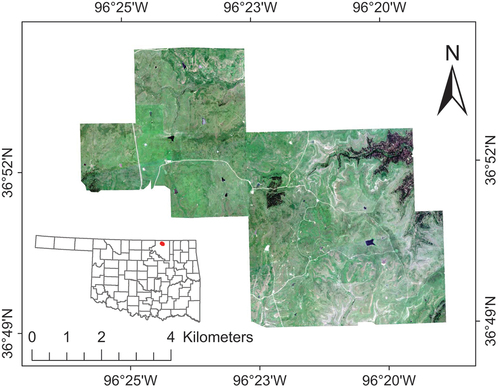
The study was conducted at the northern part of the Joseph H. Williams Tallgrass Prairie Preserve (hereafter Tallgrass Prairie Preserve; 36°50′ N and 96°25′ W), Osage County, Oklahoma, U.S., with a total area of 47 km² (Figure 1). The Tallgrass Prairie Preserve, a naturally assembled prairie, is the largest protected remnant of tallgrass on Earth (Allen et al. 2009). This site has been managed to maintain and enhance biodiversity through synergistic application of prescribed fire and grazing (Fuhlendorf and Engle 2001); however, it has also been significantly affected by L. cuneata invasion (Sherrill et al. 2022).

Figure 1. The true colour composite image of the study area within the Joseph H. Williams Tallgrass Prairie Preserve, Oklahoma, U.S. The true colour composite image is a PlanetScope dataset obtained for August 14, 2020.

2.2. Field data collection

Between late July and early August 2020, we identified 49 homogenous grassland patches, ranging from 19 to 855 m² −20 of which were dominated by L. cuneata and the rest were free of L. cuneata–where we collected 193 top-of-canopy leaf samples which were used to quantify vegetation functional traits, including total nitrogen, chlorophyll a + b, carotenoid content, and plant height. In the field, we used liquid nitrogen to immediately freeze the foliage samples and stored them on dry ice until their transfer to a −80°C freezer in the lab. We then quantified chlorophyll a + b and carotenoid content using a High Performance Liquid Chromatography (HPLC; Agilent 1200 Series, Agilent Technologies, Santa Clara, CA) at the Forest Chemical Ecology Lab, University of Wisconsin-Madison. To quantify total nitrogen content, we analysed the samples at the Soil, Water, and Forage Analytical Laboratory (SWFAL), Oklahoma State University, using a combustion analyser (Leco CN628, LECO Corporation, St. Joseph, Michigan, U.S.A.). We measured canopy height in the field using the visual obstruction technique by taking an RGB (Red Green Blue) image of grassland patches at each sampling location with a 1 × 1 m whiteboard in the background ((Limb et al. 2007); see Fig. S1 in Supplementary material). We also identified 78 independent grassland patches in the field, among which 36 patches were dominated by L. cuneata and the remaining 42 patches were free of L. cuneata. We recorded the location of all 127 patches (i.e. 49 patches used for foliar sampling and 78 L. cuneata presence/absence patches) using a GPS unit (Trimble GeoXH, Trimble, Sunnyvale, CA, U.S.A.). The area of these patches ranged from 11 to 1139 m². Field data collection was conducted within a reasonable time frame from our airborne hyperspectral data collection to minimize the impact of temporal mismatch between airborne and in situ data on our results. A complete description of data collection and data analysis protocols can be found in Gholizadeh et al. (2022).

2.3. Remote sensing datasets

Airborne hyperspectral data: We collected full-range airborne hyperspectral imagery on August 3, 2020, using a Twin Commander 500-B aircraft (Aero Commander, Oklahoma City, OK). The data have a spatial resolution of 1 m. The sensor had 323 bands ranging from 400 to 2450 nm but we used 238 bands after pre-processing and removing noisy and water vapour absorption bands (Table 1). We used airborne hyperspectral data to identify vegetation indices associated with functional traits that distinguish L. cuneata from native plants (see Section 2.4.2) and develop machine learning models to map L. cuneata (see Section 2.4.3).

Table 1. Details of the collected remote sensing imagery used in our study.

Platform	Spectral resolution	Spatial resolution	Imagery acquisition date
Twin Commander 500-B aircraft	238 bands (431.10–1299.36 nm, 1487.71–1775.03 nm, 1998.23–2353.76 nm)	1 m	08/03/2020
PlanetScope	4 bands (Blue 455–515 nm, Green 500–590 nm, Red 590–670 nm, NIR 780–860 nm)	Resampled to 3 m	05/06/2020, 05/31/2020, 06/05/2020, 06/10/2020, 06/11/2020, 06/14/2020, 08/03/2020, 08/14/2020, 09/28/2020, 09/29/2020, 09/30/2020, 10/01/2020,10/02/2020, 10/13/2020
Multitemporal PlanetScope	56 bands (4 bands × 14 dates)

PlanetScope multispectral satellite data: PlanetScope is a constellation of approximately 130 small satellites (with a size of 10 cm × 10 cm × 30 cm) owned by Planet Labs that takes almost daily imagery of the surface of the earth (Planet Labs 2022). We used Level 3B Planet imagery which were geometrically and radiometrically corrected. Level 3B is the geometrically corrected surface reflectance data generated using 6SV2.1 radiative transfer code and MODIS near-real-time data (Planet Labs 2022). We used our fine-resolution airborne imagery as reference to assess the georectification quality of our PlanetScope imagery. The airborne sensor and the navigation system of the aircraft were boresight-calibrated. Moreover, realtime differential corrections were used to maximize the accuracy of aircraft’s navigation data. Therefore, we compared all PlanetScope scenes with our fine-resolution airborne imagery as the reference. Since we did not observe any systematic geometric distortions in our PlanetScope scenes, no further geometric correction was deemed necessary. We used PlanetScope multispectral imagery with four spectral bands (Table 1), including red, green, blue, and near-infrared (NIR). The data had native spatial resolution of 3.0–4.1 m but they were resampled and delivered in 3 m images (Planet Labs 2022). Through NASA’s Commercial Smallsat Data Acquisition programme, we downloaded 14 available cloud-free PlanetScope images from May 5 to 13 October 2020. We used this time window based on approximate green-up and senescence of L. cuneata at the Tallgrass Prairie Preserve (Blair, Nippert, and Briggs 2014; Sherrill et al. 2022). We note that no imagery was available for the month of July due to cloud coverage. We used these images to determine the optimal period of the growing season to detect L. cuneata.

Multitemporal PlanetScope data cube: To assess whether a multispectral/multitemporal data cube enhances our ability to detect L. cuneata, we also combined our multitemporal PlanetScope data to produce a cube of 56 bands (4 bands × 14 dates). After producing the 56-band multitemporal data cube, we applied principal component analysis (PCA) to the stacked data cube (Ingebritsen and Lyon 1985) using the factoextra package in R (Kassambara and Mundt 2020) to reduce the dimensionality of the data and multicollinearity between spectral bands (Singh and Glenn 2009). We selected the first three PCA components that explained at least 85% of the total variance in the data (see Fig. S2 in Supplementary material).

2.4. Data analysis

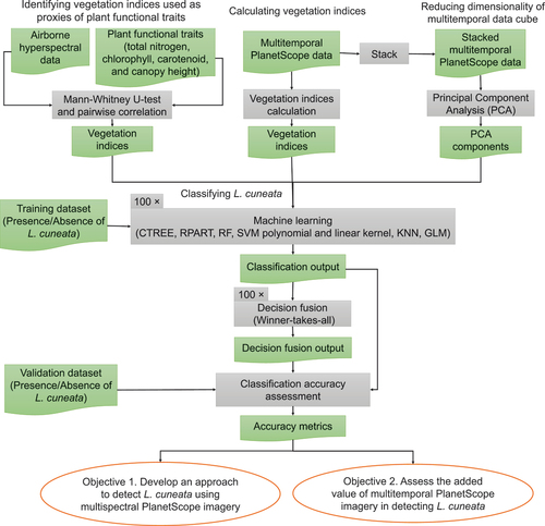
We conducted our analysis in two main steps. In step one, using the data we collected in the field and our airborne hyperspectral data, we identified vegetation indices associated with key functional traits that differentiated L. cuneata from native plants, including total nitrogen, chlorophyll a + b, carotenoid content, and plant height (Figure 2). We then developed machine learning models to separate L. cuneata from native plants using these vegetation indices as input layers. In step two, we applied our machine learning approach to our hyperspectral data, each PlanetScope multispectral data collected at different times of the growing season, and our multitemporal PlanetScope data cube. A flowchart summarizing our approach is shown in Figure 2.

Figure 2. Summary of our approach. In this flowchart, green rectangles with wavy bases represent the input/output data, grey rectangles represent the processing steps, and orange ellipses are the objectives.

2.4.1. Assessing the potential of hyperspectral data to separate L. cuneata from native plants

Using our airborne hyperspectral data, we extracted reflectance of L. cuneata and native vegetation stands from our 49 homogenous grassland patches. We conducted a Kruskal–Wallis test (Kruskal and Wallis 1952) in R program (R Core Team 2021) to compare the reflectance of L. cuneata with native plants at each band and identified wavelength regions where L. cuneata and native plants had statistically different reflectance. Identifying whether L. cuneata and native plants had significantly different reflectance values within the visible and NIR regions guided us to select the most appropriate vegetation indices to map L. cuneata.

2.4.2. Linking traits to vegetation indices

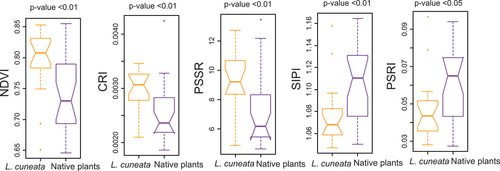
Using Mann–Whitney U test (Mann and Whitney 1947), we assessed the difference between key functional traits of L. cuneata and native plants. Specifically, we applied the Mann–Whitney U test to total nitrogen, chlorophyll a + b, carotenoid content, and canopy height from our 49 patches. We then identified vegetation indices associated with these traits by conducting a pairwise correlation analysis. Then, we assessed whether the selected vegetation indices can significantly distinguish L. cuneata from native plants using Mann–Whitney U test. Following this approach, we were able to select vegetation indices associated with underlying functional traits that distinguish L. cuneata from native plants. We tested ten vegetation indices (see Table S1 in Supplementary material) applicable to PlanetScope multispectral imagery. Out of these ten indices, we selected five indices that were able to distinguish L. cuneata from native plants. These vegetation indices included NDVI, SIPI, CRI, PSSR, and PSRI (Table 2).

Table 2. Vegetation indices used to distinguish L. cuneata from native plants. In the table below, ‘R’ represents reflectance from airborne hyperspectral imagery at different wavelengths of the electromagnetic spectrum, numbers in front of R represent wavelengths in nm, and ‘B’ represents band number from PlanetScope imagery.

Vegetation index	Formula based on airborne data	Formula based on PlanetScope bands	References
NDVI (Normalized Difference Vegetation Index)	(R800-R683) /(R800+R683)	(B4-B3) /(B4+B3)	(Rouse et al. 1974)
SIPI (Structurally Insensitive Pigment Index)	(R800-R444) /(R800-R683)	(B4-B1) /(B4-B3)	(Peñuelas, Baret, and Filella 1995)
CRI (Carotenoid Reflectance Index 2)	(1/R512)-(1/R770)	(1/B2)-(1/B4)	(Gitelson et al. 2002)
PSSR (Pigment-Specific Spectral Ratio)	R800/R635	B4/B3	(Blackburn 1998)
PSRI (Plant Senescence Reflectance Index)	(R683-R505) /R752	(B3-B2)/B4	(Merzlyak et al. 1999)

2.4.3. Developing machine learning models to detect L. cuneata using remotely sensed data

Because large number of machine learning algorithms exist, we decided to select seven algorithms ensuring that they cover different machine learning paradigms. To detect L. cuneata, we used seven supervised machine learning algorithms, including conditional inference tree (Hothorn, Hornik, and Zeileis 2006), recursive partitioning and regression trees (Clark and Pregibon 1992), random forest (Breiman 2001), support vector machine linear kernel (Cortes and Vapnik 1995), and polynomial kernel (Cortes and Vapnik 1995), k-nearest neighbours (Cover and Hart 1967; Fix and Hodges 1989), and generalized linear model (McCullagh 1983). To develop machine learning algorithms, we used the plyr and caret packages in R (Kuhn 2008; Wickham 2011). We trained the models using 10-fold cross-validation with 500 iterations. A description of each machine learning classifier along with its parameters is provided in Section S1 and Table S2 in Supplementary material.

To develop machine learning models for detecting L. cuneata, we used 60% of the 127 patches identified in the field (i.e. 49 patches used for foliar sampling and 78 L. cuneata presence/absence patches) to train the machine learning models and the rest to validate the models. We developed separate machine learning algorithms for airborne hyperspectral data, each PlanetScope multispectral dataset collected at different times of the growing season, and our multitemporal PlanetScope data cube. We applied machine learning algorithms to our hyperspectral data to assess the added value of finer spatial and spectral resolution for classifying L. cuneata.

After developing each classification model using the training dataset, we validated the models using the validation dataset (the remaining 40% of our 127 homogeneous grassland patches). Specifically, we calculated the overall classification accuracy, the balanced accuracy, the specificity, the sensitivity, the no-information rate, the producer’s and the user’s accuracy of L. cuneata for each model. A description of each accuracy metric is provided in Section S2 in Supplementary material.

We used decision fusion to combine the outputs of our seven machine learning classifiers to reduce the bias from each model in the detection of L. cuneata (Bigdeli, Samadzadegan, and Reinartz 2014). We used the winner-takes-all (WTA) to combine the output of the seven machine learning classification at each model run. WTA classification is based on the majority votes, where the class label with the most ‘votes’ is assigned to the pixel (Mancini, Frontoni, and Zingaretti 2009). To assess the performance of our WTA classifier, we used the same classification accuracy metrics mentioned above and in Section S2 in Supplementary material.

Finally, to report the uncertainty of our models, we repeated our approach 100 times through randomized permutations of our training/validation datasets. Specifically, we repeatedly selected random subsamples from our 127 homogeneous grassland patches and iteratively ran our machine learning models to detect L. cuneata in the study area. Using the results of these 100 iterations, instead of producing one binary presence/absence map, we generated a probability presence map of L. cuneata. We note that we excluded the oak tree non-grassland land-cover from our analysis.

3. Results

3.1. Assessing differences between the spectral signature of L. cuneata and native plants

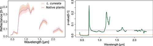
Our results showed that compared to native plants, L. cuneata, in general, had higher spectral reflectance in the NIR region and lower reflectance in other regions of the electromagnetic spectrum (Figure 3a). Based on the Kruskal–Wallis test, L. cuneata and the native plants had significantly different spectral reflectance, particularly in the visible range of the electromagnetic spectrum (p-value <0.05 for the reflectance at 400–700 nm) and large portions of the NIR region (p-value <0.05 for the reflectance at 800–1100 nm; Figure 3b).

Figure 3. (a) Spectral signatures of L. cuneata and native plants from our airborne hyperspectral data. Shaded regions show the standard deviation of spectra. (b) Statistical difference between the reflectance of L. cuneata and native plants based on Kruskal-Wallis test (green line). The upper purple dashed line shows the p-value at 0.05, and the lower orange dashed line shows the p-value at 0.01.

3.2. Using vegetation indices as proxies of plant functional traits to detect L. cuneata

Using Mann–Whitney U test, our results showed that L. cuneata had higher total nitrogen, canopy height, chlorophyll, and carotenoid content than native plants (see Fig. S3 in Supplementary material), a result which was also reported in Gholizadeh et al. (2022). Pairwise correlation values between functional traits and vegetation indices showed significant associations (p-value <0.05), except for the correlation between CRI and chlorophyll content (Figure 4). Additionally, based on Mann–Whitney U test, the selected vegetation indices were able to differentiate L. cuneata from native plants (p-value <0.05; Figure 5).

Figure 4. Pairwise correlations between vegetation indices derived from our airborne hyperspectral data and functional traits measured in the field. The circle sizes are proportional to the correlation coefficients, which are represented by the numbers shown inside each circle. The red asterisks show significant correlations (p-value <0.05). Vegetation index acronyms: NDVI: normalized difference vegetation Index, CRI: carotenoid reflectance Index, PSSR: pigment-specific spectral Ratio, SIPI: structurally insensitive Pigment Index, and PSRI: plant senescence reflectance Index.

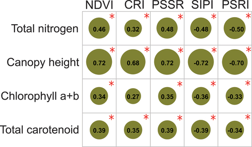
Figure 5. Differences in vegetation indices for L. cuneata versus native plants using the Mann-Whitney U test based on our airborne hyperspectral data. Significant differences in vegetation indices indicate the ability of these indices in distinguishing L. cuneata from native plants. Vegetation index acronyms: NDVI: normalized difference vegetation Index, CRI: carotenoid reflectance Index, PSSR: pigment-specific spectral Ratio, SIPI: structurally insensitive Pigment Index, and PSRI: plant senescence reflectance Index.

3.3. Detecting L. cuneata using machine learning

Classification accuracy assessment on the validation dataset showed that the overall classification accuracy using our airborne hyperspectral data ranged from 79.30 ± 4.99% (using RF) to 81.62 ± 3.85% (using SVM linear kernel; Table 3). Our results showed that the overall classification accuracy in detecting L. cuneata using the developed machine learning models exceeded the no-information rate value (Table 3).

Table 3. Classification accuracy metrics for detecting L. cuneata in the airborne hyperspectral data using our seven machine learning models and our WTA decision fusion approach based on the validation dataset. In the table below, no-information rate corresponds to the rate that should be exceeded to have an ‘accurate’ classification. Overall accuracy represents the ratio of the correctly classified class over the total dataset. Balanced accuracy refers to the average value of sensitivity, defined as the accuracy in predicting the absence of L. cuneata in the map, and the specificity, defined as the accuracy in predicting the presence of L. cuneata in the map. Producer’s accuracy refers to how well the presence of L. cuneata on the ground can be mapped, and user’s accuracy refers to how well the classified L. cuneata map represents L. cuneata on the ground.

	CTREE	RPART	RF	SVM linear	SVM polynomial	KNN	GLM	WTA
No-information rate (%)	56.01± 3.97	56.01± 3.97	56.01± 3.97	56.01± 3.97	56.01± 3.97	56.01± 3.97	55.90± 4.22	56.05± 4.03
Overall accuracy (%)	80.16± 4.14	81.42± 4.12	79.30± 4.99	81.62± 3.85	8.85± 4.66	79.63± 5.15	79.81± 5.54	81.86± 4.12
Balanced accuracy (%)	80.71± 4.24	81.92± 4.15	79.44± 5.12	81.81± 4.00	81.25± 4.68	79.88± 5.15	80.04± 5.51	82.19± 4.28
Sensitivity (%)	76.49± 7.82	77.43± 6.99	79.58± 7.41	81.43± 6.68	79.37± 7.36	78.67± 7.78	79.85± 8.12	80.01± 6.72
Specificity (%)	84.92± 8.24	86.41± 6.26	79.30± 9.10	82.18± 7.51	83.13± 7.45	81.09± 9.47	80.22± 8.02	84.37± 7.08
L. cuneata producer’s accuracy (%)	84.92± 8.22	86.41± 6.27	79.30± 9.10	82.18± 7.51	83.13± 7.45	81.09± 9.48	80.22± 8.02	84.37± 7.08
L. cuneata user’s accuracy (%)	74.96± 7.09	75.90± 6.96	76.19± 7.67	78.47± 6.94	76.73± 7.94	75.96± 7.76	77.35± 8.69	77.62± 6.85

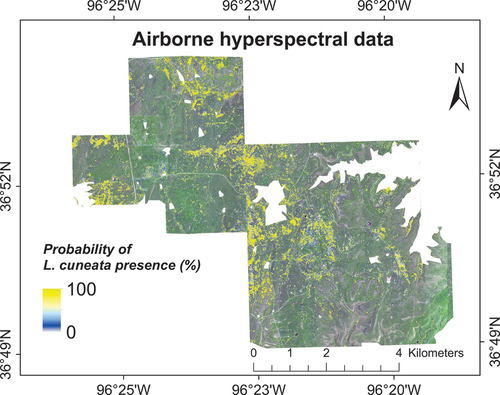
Nevertheless, our results showed that the performance of machine learning algorithms was not the same, but fusing the outcomes of various machine learning algorithms always showed performance comparable to that of the best classifier. Specifically, our WTA decision fusion had an overall classification accuracy of 81.86 ± 4.12%, producer’s accuracy of 84.37 ± 7.08%, and user’s accuracy of 77.62 ± 6.85% using our validation dataset (Table 3). Classification using our airborne hyperspectral showed that L. cuneata had invaded at least 6.23% of our study area (Figure 6).

Figure 6. Probability of L. cuneata presence using vegetation indices obtained from airborne hyperspectral image based on our WTA classification. We obtained these results by running our classification models 100 times with different training/validation datasets through randomized permutations, as described in Section 2.4.4. We excluded the oak tree land-cover from our results.

3.4. Identifying the best periods of the growing season to detect L. cuneata

We detected L. cuneata for each PlanetScope image collected during the growing season to identify optimal time periods for separating L. cuneata from native plants (Figure 7). Based on our validation data, the overall classification accuracy at the start of the growing season was relatively low. Only GLM and SVM classifiers showed an overall classification accuracy higher than the no-information rate at the start of the growing season.

Figure 7. Average overall classification accuracy in detecting L. cuneata during the growing season using seven machine learning classifiers (CTREE, KNN, RF, SVM polynomial kernel, SVM linear kernel, GLM, RPART) and WTA decision fusion approach. The dashed black line shows the average of the no-information rate value for each DoY. We obtained these results by running our machine learning models 100 times with different training/validation datasets through randomized permutations. Note that we were not able to assess the performance of our model in July due to cloud coverage in our PlanetScope imagery.

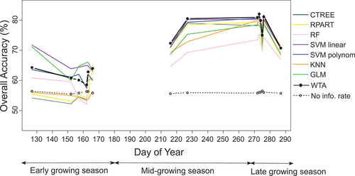
Starting from DoY (day of year) 216, the overall classification accuracy in detecting L. cuneata for all the classifiers was higher than the no-information rate (Figure 7). The value ranged from 66.62 ± 7.73% (DoY 216 using RF) to 81.63 ± 5.99% (DoY 276 using SVM polynomial kernel). During the same time period (after DoY 216), the user’s accuracy was lowest at DoY 287 (63.77 ± 8.73% using CTREE) and highest at DoY 273 (81.63 ± 10.79% using SVM linear kernel). Following a similar pattern, the producer’s accuracy was lowest at DoY 287 (60.00 ± 12.17% using RF) and was highest at DoY 273 (80.57 ± 7.35% using KNN).

During the mid-growing season, our WTA decision fusion classification showed an improved overall classification accuracy in detecting L. cuneata compared to the seven classifiers developed for this study. The overall classification accuracy using WTA decision fusion ranged from 58.58 ± 7.61% (DoY 162) to 82.02 ± 4.66% (DoY 273). The user’s accuracy value ranged from 58.65 ± 12.46% (DoY 157) to 81.01 ± 8.78% (DoY 273), while the producer’s accuracy value ranged from 41.02 ± 18.66% (DoY 152) to 79.49 ± 8.65% (DoY 272).

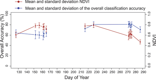
Although our WTA decision fusion improved our classification accuracy results, the overall classification accuracy in detecting L. cuneata remained relatively low at the start of the growing season. Around the peak of the growing season at DoY 227 (NDVI value of 0.79 ± 0.04), the overall classification accuracy of L. cuneata was 80.49 ± 5.69%. Around the end of the growing season at DoY 273 (NDVI value of 0.60 ± 0.07), the overall classification accuracy was the highest (82.02 ± 4.66%). At the beginning of the senescence period at DoY 287 (NDVI value of 0.46 ± 0.04), the overall classification accuracy decreased to 70.74 ± 5.48% (Figure 8).

Figure 8. Overall L. cuneata classification accuracy (mean and standard deviation value) using the WTA decision fusion (blue line). The dark red line shows the mean and standard deviation of NDVI during the growing season, which represents the plant greenness. We obtained these results by running our machine learning models 100 times with different training/validation datasets through randomized permutations. Note that we were not able to assess the performance of our models in July due to cloud coverage in our PlanetScope imagery.

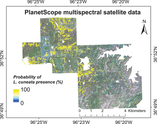
We mapped the probability of L. cuneata presence on August 14, 2020, the peak of the growing season (Figure 9). The results showed a comparatively similar map to that obtained from the airborne hyperspectral imagery collected on August 3, 2020. Similar to our findings using airborne hyperspectral imagery, our results showed that at least 6.83% of our study area had been invaded by L. cuneata.

Figure 9. Probability of L. cuneata presence using vegetation indices obtained from PlanetScope multispectral image at the peak of the growing season (DoY 227) based on our WTA classification. We obtained these results by running our classification models 100 times with different training/validation datasets through randomized permutations. We excluded the oak tree land-cover from our results.

3.5. Determining the contribution of combined multitemporal PlanetScope imagery in detecting L. cuneata

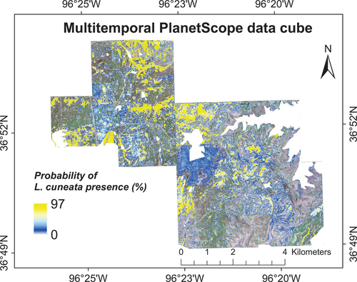
Using the first three components of our multitemporal PlanetScope data cube as input layers to our machine learning approach, we were able to detect L. cuneata. Specifically, while no-information rate in detecting L. cuneata was 60.73 ± 7.22%, our overall classification accuracy based on WTA decision fusion was 69.26 ± 8.45%, with a user’s accuracy of 76.29 ± 19.11% and a producer’s accuracy of 41.51 ± 17.83%. These results suggest that L. cuneata and native plants presumably have different phenology that was captured by the PCA of our data cube. However, while previous maps using vegetation indices had identified pixels with 100% probability of L. cuneata presence (Figure 6 and 9), the highest probability for L. cuneata presence using PCA approach was 97% (Figure 10).

Figure 10. Probability of L. cuneata presence based on WTA decision fusion using three PCA components obtained from the combined multitemporal PlanetScope imagery. We obtained these results by running our classification models 100 times with different training/validation datasets through randomized permutations. We excluded oak tree land-cover from our results.

4. Discussion

4.1. Mapping grassland invasive plants using vegetation indices

Hyperspectral remote sensing has been identified as a viable tool to map invasive plants in grasslands (Arasumani et al. 2021; Bolch et al. 2020; Hestir et al. 2008; Huang et al. 2021; Niphadkar and Nagendra 2016; Underwood 2003). However, due to the high acquisition and computational cost of hyperspectral remote sensing and limited access to airborne hyperspectral data, we developed an approach to detect the invasive L. cuneata for multispectral data based on vegetation indices. While using vegetation indices to distinguish different land-cover types or species is not new (Lyon et al. 1998), our approach was based on the fact that there are remotely observable plant functional traits that can separate invasive from native plants (Underwood, Ustin, and Ramirez 2007; Asner et al. 2008). Therefore, we used multispectral vegetation indices as proxies of these plant functional traits to increase the transferability and generalizability of our approach. Our approach showed lower overall classification accuracy for detecting L. cuneata compared to previous studies which used airborne hyperspectral data (Gholizadeh et al. 2022). The lower detection accuracy of our approach is likely due to our use of vegetation indices estimated using only two to three spectral bands, while Gholizadeh et al. (2022) used remotely observable plant functional traits estimated using more than 200 spectral bands. Moreover, vegetation indices do not estimate traits directly but are proxies of these traits. Nevertheless, our results showed that detecting L. cuneata using PlanetScope multispectral data is feasible, presumably because of selection of relevant vegetation indices that are associated with key functional traits that separate L. cuneata from native plants.

Although our approach had lower classification accuracy compared to the results obtained from fine-resolution airborne hyperspectral data in Gholizadeh et al. (2022), our classification accuracy remained higher than the no-information rate (see Table 3), indicating that our approach offers a cost-effective alternative to detecting invasive plants using hyperspectral data, especially given the transferability and generalizability of our approach. Specifically, airborne hyperspectral data acquisition at our site cost approximately US$60,000, while PlanetScope imagery of the same site cost US$500. If the available funding for acquiring PlanetScope data was US$60,000, these data would have covered roughly 19,000 km² more area than airborne hyperspectral imagery. Therefore, in addition to its ecological and conservation benefits, our study can have significant economic benefits, especially when controlling the spread of invasive plants in grasslands represents one of the greatest land management costs. Through providing an iterative, scalable, and cost-effective monitoring system, our approach can assist landowners with locating priority area for early intervention and, thereby, reduce the costs of invasion control.

4.2. Advantages of fine spatial and temporal resolution in detecting biological invasions

Our results showed the superior performance of airborne hyperspectral data in mapping invasive plants in terms of producer’s accuracy (see Table 3 and Section 3.4) because of the finer spatial resolution of our airborne data. Nevertheless, our results showed that multispectral PlanetScope data were capable of mapping L. cuneata accurately when applied at optimal times of the growing season. This result agrees with findings of Mullerova et al. (2017) indicating that selecting optimal timing can compensate for the coarse spectral resolution of satellite-derived data in detecting invasive species.

Fine temporal resolution of PlanetScope imagery can also contribute to identifying distinct phenological patterns of invasive versus native plants, which in turn, enhances the accuracy of mapping invasive plants. Previous studies using multitemporal PlanetScope imagery for mapping invasive species, such as Euphorbia esula (leafy spurge) (Lake et al. 2022) and Spartina alterniflora (saltmarshes cordgrass) (Han et al. 2022) have shown the added value of PlanetScope multitemporal imagery through providing information on plant phenology. Similarly, our results showed that PlanetScope data can separate L. cuneata from native plants, and identify optimal periods of the growing season to detect its spread, as described in Section 4.3 below.

4.3. Importance of the timing of remote sensing data collection in mapping biological invasions

Our findings indicated that the optimal period to detect L. cuneata at the Tallgrass Prairie Preserve was near the peak and towards the end of the growing season. The peak of the growing season corresponds to the period when plants form a full canopy and when the difference between the spectral signatures of invasive and native plants, in general, is maximized (Dao, Axiotis, and He 2021). Our results also showed high overall classification accuracy towards the end of the growing season. Although the NDVI values of native and invasive plants were not significantly different at the end of the growing season (see Fig. S4 in Supplementary material), the average NDVI values of L. cuneata were higher than those of the native plants (see Fig. S4 in Supplementary material). These results suggest that L. cuneata may have remained green (i.e. photosynthetically active) longer than native plants, which presumably increased the detection accuracy of L. cuneata at the end of the growing season. Similar findings have been reported in Evangelista et al. (2009), showing that the detection accuracy of Tamarisk spp. (tamarix) was highest during the peak of the growing season and flowering period (June) and around the start of the senescence period (September and October). While our results identified the peak and the end of the growing season as optimal time periods to detect L. cuneata, we acknowledge that the optimal time periods for remote detection of invasive plants is species-specific. For instance, while Tuanmu et al. (2010) mapped Bashania faberi and Fargesia robusta (bamboo species) during the early stages of the growing season and during the senescence period, Lake et al. (2022) showed that Euphorbia esula (leafy spurge) was best detected during the early and mid-growing season. We also acknowledge that plant phenology can change in response to environmental conditions, such as precipitation and temperature, which further complicates remote monitoring of invasive plants. Therefore, incorporating environmental variables with remote sensing observations can be a promising approach to improve monitoring biological invasions.

4.4. Limitations

4.4.1. Temporal mismatch between in situ and remotely sensed data collection campaigns

Our results showed that the detection accuracy of L. cuneata at the start of the growing season was relatively low. In our study, we used ground-reference data collected at the peak of the growing season to identify L. cuneata at different periods of the growing season. This temporal mismatch may have affected the performance of our approach at the beginning of the growing season. Cummings et al. (2007) reported that new germination of L. cuneata generally occurs between early April and June in Oklahoma (Cummings et al. 2007). Therefore, the homogeneous patches that we sampled during the peak of the growing season may not fully represent L. cuneata patches at the start of the growing season.

Another plausible reason for the low detection accuracy of L. cuneata at the start of the growing season is that we identified functional trait differences based on the foliage samples collected during the peak of the growing season. In other words, we used plant traits collected during the peak of the growing season to identify suitable vegetation indices and applied the same vegetation indices to our data collected at different times of the growing season. To reduce the impact of this uncertainty, we encourage multitemporal field data collection campaigns when possible.

4.4.2. Spatial mismatch between plant size and pixel size

The degree to which remote sensing methods can detect invasive species depends on the size of the individual plant or the dimensions of stands they form with respect to the spatial resolution of remote sensing data. For grassland ecosystems, it is unlikely for spaceborne remote sensing data, such as PlanetScope, to detect individual plants (see Fig. S5 in Supplementary material) or map sparse patches of invasive plants mixed with native species. Given the limited spatial resolution of available spaceborne platforms, using finer-resolution multispectral data, for example, those collected using unoccupied aircraft systems, can provide an exciting opportunity to assess the sensitivity of our approach to sparse or mixed vegetation communities.

5. Conclusions

This study aimed to map the invasive L. cuneata in a naturally assembled grassland using multispectral multitemporal remotely sensed data. We first used airborne hyperspectral data to identify vegetation indices associated with key functional trait differences that separated L. cuneata from native plants. We then applied these vegetation indices to PlanetScope multispectral data to map L. cuneata over the growing season. Our approach showed that PlanetScope data were capable of detecting L. cuneata although the accuracy of detection varied based on the timing of the imagery used. We also recorded a high classification accuracy at the peak of the growing season, with our best classification accuracy achieved towards the end of the season. Overall, our results showed that although we used the 4-band PlanetScope multispectral data, our classification accuracy results were comparable to those obtained from hyperspectral data with fine spatial and spectral resolution. These findings can contribute to developing cost-effective approaches for monitoring invasive plants in grasslands across large geographical extents and over the growing season. Our results demonstrate that available satellite multispectral imagery can be used to map invasive species and offer an approach to develop effective and science-driven management practices to control the spread of invasive plants in grassland ecosystems and mitigate the impacts of biological invasions.

Acknowledgements

We sincerely thank the two anonymous reviewers who helped us improve the quality of our manuscript. We also express our sincere gratitude to Michael S. Friedman, Nicholas McMillan, Aisha Sams, Makyla Charles, and DeAndre Garrett who helped us at the early stages of this project. We thank The Nature Conservancy for facilitating the study. M. Ny Aina Rakotoarivony was partially supported by the Delores and Jerry Etter Graduate Research Program and the J.E. Weaver Competitive Grants Program. Hamed Gholizadeh was supported by a NASA NIP award [80NSSC21K0941].

Disclosure statement

No potential conflict of interest was reported by the author(s).

Data availability statement

Processed full-range 1-m airborne hyperspectral data are available to download free of charge from the NASA EOSDIS Land Processes Distributed Active Archive Center at https://lpdaac.usgs.gov/products/aehyp1tppokv001/.

Supplementary material

Supplemental data for this article can be accessed online at https://doi.org/10.1080/01431161.2023.2275321.

Additional information

Funding

Data collection and analysis efforts were supported through The Oklahoma Center for the Advancement of Science and Technology (OCAST) Basic Plant Science Research program [grant number PS20-004 to H.G.], National Aeronautics and Space Administration (NASA) NIP award [grant number 80NSSC21K0941 to H.G.], United States Department of Agriculture (USDA) NIFA program [grant number 2019-68012-29819 to S.F.], National Science Foundation (NSF) Division of Biological Infrastructure [grant number DBI 2021898 to A.T.], the Delores and Jerry Etter Graduate Research Scholarship and the J.E. Weaver Competitive Grants Program to M.N.A.R., NSF GRFP program [grant number 1-653428 to W.H.], USDA NIFA program [McIntire Stennis project number 1019284 to H.A.], and Groendyke Endowment to S.F.

References

- Allen, M. S., R. G. Hamilton, U. Melcher, and M. W. Palmer. 2009. Lessons from the Prairie: Research at the Nature Conservancy’s Tallgrass Prairie Preserve. Stillwater, Oklahoma: Oklahoma Academy of Sciences.
- Anderson, R. C. 2006. “Evolution and Origin of the Central Grassland of North America: Climate, Fire, and Mammalian Grazers1.” Journal of the Torrey Botanical Society 133 (4): 626–647. https://doi.org/10.3159/1095-5674(2006)133[626:Eaootc]2.0.Co;2.
- Arasumani, M., A. Singh, M. Bunyan, and V. V. Robin. 2021. “Testing the Efficacy of Hyperspectral (AVIRIS-NG), Multispectral (Sentinel-2) and Radar (Sentinel-1) Remote Sensing Images to Detect Native and Invasive Non-Native Trees.” Biological Invasions 23 (9): 2863–2879. https://doi.org/10.1007/s10530-021-02543-2.
- Asner, G. P., M. O. Jones, R. E. Martin, D. E. Knapp, and R. F. Hughes. 2008. “Remote Sensing of Native and Invasive Species in Hawaiian Forests.” Remote Sensing of Environment 112 (5): 1912–1926. https://doi.org/10.1016/j.rse.2007.02.043.
- Bartz, R., and I. Kowarik. 2019. “Assessing the Environmental Impacts of Invasive Alien Plants: A Review of Assessment Approaches.” NeoBiota 43:69–99. https://doi.org/10.3897/neobiota.43.30122.
- Bengtsson, J., J. M. Bullock, B. Egoh, C. Everson, T. Everson, T. O’Connor, P. J. O’Farrell, H. G. Smith, and R. Lindborg. 2019. “Grasslands—More Important for Ecosystem Services Than You Might Think.” Ecosphere 10 (2): 20.
- Bigdeli, B., F. Samadzadegan, and P. Reinartz. 2014. “A Decision Fusion Method Based on Multiple Support Vector Machine System for Fusion of Hyperspectral and LIDAR Data.” International Journal of Image and Data Fusion 5 (3): 196–209. https://doi.org/10.1080/19479832.2014.919964.
- Blackburn, G. A. 1998. “Spectral Indices for Estimating Photosynthetic Pigment Concentrations: A Test Using Senescent Tree Leaves.” International Journal of Remote Sensing 19 (4): 657–675.
- Blair, J., J. Nippert, and J. Briggs. 2014. Grassland Ecology. In Ecology and the Environment, edited by Monson R.K. Ecology and the Environment 8:389–423. New York: Springer Science.
- Bolch, E. A., M. J. Santos, C. Ade, S. Khanna, N. T. Basinger, M. O. Reader, and E. L. Hestir. 2020. Remote detection of invasive alien species.In Remote Sensing of Plant Biodiversity, edited by, 267–307. New York: Springer Nature.
- Bradley, B. A., and J. F. Mustard. 2005. “Identifying Land Cover Variability Distinct from Land Cover Change: Cheatgrass in the Great Basin.” Remote Sensing of Environment 94 (2): 204–213. https://doi.org/10.1016/j.rse.2004.08.016.
- Breiman, L. 2001. “Random Forest.” Machine Learning 45:5–32.
- Cheng, Y., A. Vrieling, F. Fava, M. Meroni, M. Marshall, and S. Gachoki. 2020. “Phenology of Short Vegetation Cycles in a Kenyan Rangeland from PlanetScope and Sentinel-2.” Remote Sensing of Environment 248. https://doi.org/10.1016/j.rse.2020.112004.
- Chen, B., Y. Jin, and P. Brown. 2019. “An Enhanced Bloom Index for Quantifying Floral Phenology Using Multi-Scale Remote Sensing Observations.” Isprs Journal of Photogrammetry & Remote Sensing 156:108–120. https://doi.org/10.1016/j.isprsjprs.2019.08.006.
- Clark, L. A., and D. Pregibon. 1992. “Tree-Based Models.” In Statistical Models in S, edited by J. M. Chambers and T. J. Hastie. Pacific Grove, CA: Wadsworth and Brooks/Cole. 377–419.
- Cortes, C., and V. Vapnik. 1995. “Support-Vector Networks.” Machine Learning 20:273–297. https://doi.org/10.1007/BF00994018.
- Cover, T., and P. Hart. 1967. “Nearest Neighbor Pattern Classification.” IEEE Transactions on Information Theory 13 (1): 21–27.
- Cummings, C., T. G. Bidwell, C. R. Medlin, S. D. Fuhlendorf, R. D. Elmore, and J. R. Weir. 2007. “Ecology and Management of Sericea Lespedeza.” Oklahoma Cooperative Extension Service. NREM 2874:7.
- Dao, P. D., A. Axiotis, and Y. He. 2021. “Mapping Native and Invasive Grassland Species and Characterizing Topography-Driven Species Dynamics Using High Spatial Resolution Hyperspectral Imagery.” International Journal of Applied Earth Observation and Geoinformation 104. https://doi.org/10.1016/j.jag.2021.102542.
- DiTomaso, J. M. 2000. “Invasive Weeds in Rangelands: Species, Impacts and Management.” Weed Science 48 (2): 255–265.
- Evangelista, P., T. Stohlgren, J. Morisette, and S. Kumar. 2009. “Mapping Invasive Tamarisk (Tamarix): A Comparison of Single-Scene and Time-Series Analyses of Remotely Sensed Data.” Remote Sensing 1 (3): 519–533. https://doi.org/10.3390/rs1030519.
- Fantle-Lepczyk, J. E., P. J. Haubrock, A. M. Kramer, R. N. Cuthbert, A. J. Turbelin, R. Crystal-Ornelas, C. Diagne, and F. Courchamp. 2022. “Economic Costs of Biological Invasions in the United States.” Science of the Total Environment 806 (Pt 3): 151318. https://doi.org/10.1016/j.scitotenv.2021.151318.
- Fix, E., and J.L. Hodges. 1989. ”Discriminatory Analysis-Nonparametric Discrimination: Consistency Properties.“ International Statistical Institute (ISI) Technical Report 57 (3): 238–247.
- Fuhlendorf, S. D., and D. M. Engle. 2001. “Restoring Heterogeneity on Rangelands: Ecosystem Management Based on Evolutionary Grazing Patterns.” Bioscience 51 (8): 625–632.
- Gholizadeh, H., M. S. Friedman, N. A. McMillan, W. M. Hammond, K. Hassani, A. V. Sams, M. D. Charles, et al. 2022. “Mapping Invasive Alien Species in Grassland Ecosystems Using Airborne Imaging Spectroscopy and Remotely Observable Vegetation Functional Traits.” Remote Sensing of Environment 271. https://doi.org/10.1016/j.rse.2022.112887.
- Gitelson, A. A., Y. Zur, O. B. Chivkunova, and M. N. Merzlyak. 2002. “Assessing Carotenoid Content in Plant Leaves with Reflectance Spectroscopy.” Photochemistry and Photobiology 75 (3): 272–281.
- Hacker, P. W., and N. C. Coops. 2022. “Using Leaf Functional Traits to Remotely Detect Cytisus Scoparius (Linnaeus) Link in Endangered Savannahs.” NeoBiota 71:149–164. https://doi.org/10.3897/neobiota.71.76573.
- Han, X., Y. Wang, Y. Ke, T. Liu, and D. Zhou. 2022. “Phenological Heterogeneities of Invasive Spartina Alterniflora Salt Marshes Revealed by High-Spatial-Resolution Satellite Imagery.” Ecological Indicators 144. https://doi.org/10.1016/j.ecolind.2022.109492.
- He, K. S., D. Rocchini, M. Neteler, and H. Nagendra. 2011. “Benefits of Hyperspectral Remote Sensing for Tracking Plant Invasions.” Diversity & Distributions 17 (3): 381–392. https://doi.org/10.1111/j.1472-4642.2011.00761.x.
- Hestir, E. L., S. Khanna, M. E. Andrew, M. J. Santos, J. H. Viers, J. A. Greenberg, S. S. Rajapakse, and S. L. Ustin. 2008. “Identification of Invasive Vegetation Using Hyperspectral Remote Sensing in the California Delta Ecosystem.” Remote Sensing of Environment 112 (11): 4034–4047. https://doi.org/10.1016/j.rse.2008.01.022.
- Hothorn, T., K. Hornik, and A. Zeileis. 2006. “Unbiased Recursive Partitioning: A Conditional Inference Framework.” Journal of Computational and Graphical Statistics 15 (3): 651–674. https://doi.org/10.1198/106186006x133933.
- Huang, C. Y., and G. P. Asner. 2009. “Applications of Remote Sensing to Alien Invasive Plant Studies.” Sensors (Basel) 9 (6): 4869–4889. https://doi.org/10.3390/s90604869.
- Huang, Y., J. Li, R. Yang, F. Wang, Y. Li, S. Zhang, F. Wan, X. Qiao, and W. Qian. 2021. “Hyperspectral Imaging for Identification of an Invasive Plant Mikania Micrantha Kunth.” Frontiers in Plant Science 12:626516. https://doi.org/10.3389/fpls.2021.626516.
- Hunt Jr, E.R.,, J. E. McMurtrey III, A. E. P. Williams, and L. A. Corp. 2004. “Spectral Characteristics of Leafy Spurge (Euphorbia Esula) Leaves and Flower Bracts.” Weed Science 52 (4): 492–497. https://doi.org/10.1614/ws-03-132r.
- Ingebritsen, S. E., and R. J. P. Lyon. 1985. “Principal Components Analysis of Multitemporal Image Pairs.” International Journal of Remote Sensing 6 (5): 687–696. https://doi.org/10.1080/0143116850894849.
- John, A., J. Ong, E. J. Theobald, J. D. Olden, A. Tan, and J. HilleRislambers. 2020. “Detecting Montane Flowering Phenology with CubeSat Imagery.” Remote Sensing 12 (18). https://doi.org/10.3390/rs12182894.
- Kassambara, A., and F. Mundt. 2020. “Factoextra: Extract and Visualize the Results of Multivariate Data Analyses.” R Package Version 1.0.7.
- Klein, P., and C. M. Smith. 2020. “Invasive Johnsongrass, a Threat to Native Grasslands and Agriculture.” Biologia 76 (2): 413–420. https://doi.org/10.2478/s11756-020-00625-5.
- Kruskal, W. H., and W. A. Wallis. 1952. “Use of Ranks in One-Criterion Variance Analysis.” Journal of the American Statistical Association 47 (260): 583–621.
- Kuhn, M. 2008. “Building Predictive Models in R Using the Caret Package.” Journal of Statistical Software 28 (5): 1–26. https://doi.org/10.18637/jss.v028.i05.
- Kumar Rai, P., and J. S. Singh. 2020. “Invasive Alien Plant Species: Their Impact on Environment, Ecosystem Services and Human Health.” Ecological Indicators 111:106020. https://doi.org/10.1016/j.ecolind.2019.106020.
- Lake, T. A., R. D. Briscoe Runquist, D. A. Moeller, T. Sankey, and Y. Ke. 2022. “Deep Learning Detects Invasive Plant Species Across Complex Landscapes Using Worldview‐2 and Planetscope Satellite Imagery.” Remote Sensing in Ecology and Conservation. https://doi.org/10.1002/rse2.288.
- Limb, R. F., K. R. Hickman, D. M. Engle, J. E. Norland, and S. D. Fuhlendorf. 2007. “Digital Photography: Reduced Investigator Variation in Visual Obstruction Measurements for Southern Tallgrass Prairie.” Rangeland Ecology and Management 60 (5): 548–552.
- Lyon, J. G., D. Yuan, R. S. Lunetta, and C. D. Elvidge. 1998. “A Change Detection Experiment Using Vegetation Indices.” Photogrammetric Engineering & Remote Sensing 64 (2): 143–150.
- Mancini, A., E. Frontoni, and P. Zingaretti. 2009. “A Winner Takes All Mechanism for Automatic Object Extraction from Multi-Source Data.” IEEE. 2009 17th International Conference on Geoinformatics. August 12-14, 2009. Fairfax, Virginia, US. 1–6.
- Mann, H. B., and D. R. Whitney. 1947. “On a Test of Whether One of 2 Random Variables is Stochastically Larger Than the Other.” Annals of Mathematical Statistics 18 (1): 50–60.
- McCullagh, P. 1983. Generalized Linear Models. Edited by Chapman and Hall. 2nd ed. London: Routledge.
- Merzlyak, M. N., A. A. Gitelson, O. B. Chivkunova, and V. Y. U. Rakitin. 1999. “Non-Destructive Optical Detection of Pigment Changes During Leaf Senescence and Fruit Ripening.” Physiologia plantarum 106 (1): 135–141.
- Moon, M., A. D. Richardson, and M. A. Friedl. 2021. “Multiscale Assessment of Land Surface Phenology from Harmonized Landsat 8 and Sentinel-2, PlanetScope, and PhenoCam Imagery.” Remote Sensing of Environment 266. https://doi.org/10.1016/j.rse.2021.112716.
- Mullerova, J., J. Bruna, T. Bartalos, P. Dvorak, M. Vitkova, and P. Pysek. 2017. “Timing is Important: Unmanned Aircraft Vs. Satellite Imagery in Plant Invasion Monitoring.” Frontiers in Plant Science 8:887. https://doi.org/10.3389/fpls.2017.00887.
- Niphadkar, M., and H. Nagendra. 2016. “Remote Sensing of Invasive Plants: Incorporating Functional Traits into the Picture.” International Journal of Remote Sensing 37 (13): 3074–3085. https://doi.org/10.1080/01431161.2016.1193795.
- Ohlenbush, P. D., T. Bidwell, W. H. Fick, G. Kilgore, W. Scott, J. Davidson, S. Clubine, J. Mayo, and M. Coffin. 2001. ”Sericea Lespedeza: History, Characteristics and Identification.” publication MF-2408. Manhattan, KS, USA: Kansas State University Agricultural Experiment. Station and Cooperative Extension Service.
- Peñuelas, J., F. Baret, and I. Filella. 1995. “Semi-Empirical Indices to Assess Carotenoids/Chlorophyll a Ratio from Leaf Spectral Reflectance.” Photosynthetica 31 (2): 221–230.
- Peterson, E. B. 2005. “Estimating Cover of an Invasive Grass (Bromus tectorum) Using Tobit Regression and Phenology Derived from Two Dates of Landsat ETM+ Data.” International Journal of Remote Sensing 26 (12): 2491–2507. https://doi.org/10.1080/01431160500127815.
- Planet Labs, P. B. C. 2022. Planet Imagery Product Specifications. San Francisco, California: PLANET.COM.
- Pysek, P., P. E. Hulme, D. Simberloff, S. Bacher, T. M. Blackburn, J. T. Carlton, W. Dawson, et al. 2020. “Scientists’ Warning on Invasive Alien Species.” Biological Reviews of the Cambridge Philosophical Society 95 (6): 1511–1534. https://doi.org/10.1111/brv.12627.
- R Core Team. 2021. R: A Language and Environment for Statistical Computing. R Foundation for Statistical Computing. https://www.R-project.org/.
- Resasco, J., A. N. Hale, M. C. Henry, and D. L. Gorchov. 2007. “Detecting an Invasive Shrub in a Deciduous Forest Understory Using Late‐Fall Landsat Sensor Imagery.” International Journal of Remote Sensing 28 (16): 3739–3745. https://doi.org/10.1080/01431160701373721.
- Rouse, J. W., R. H. Haas, D. W. Deering, J. A. Schell, and J. C. Harlan. 1974. “Monitoring the Vernal Advancement and Retrogradation (Green Wave Effect) of Natural Vegetation.” Final Rep. RSC 1978-4. Remote Sensing Center, Texas A&M Univ: College Station.
- Scholtz, R., and D. Twidwell. 2022. “The Last Continuous Grasslands on Earth: Identification and Conservation Importance.” Conservation Science and Practice 4 (3). https://doi.org/10.1111/csp2.626.
- Sherrill, C. W., S. D. Fuhlendorf, L. E. Goodman, R. D. Elmore, and R. G. Hamilton. 2022. “Managing an Invasive Species While Simultaneously Conserving Native Plant Diversity.” Rangeland Ecology & Management 80:87–95. https://doi.org/10.1016/j.rama.2021.11.001.
- Singh, N., and N. F. Glenn. 2009. “Multitemporal Spectral Analysis for Cheatgrass (Bromus tectorum) Classification.” International Journal of Remote Sensing 30 (13): 3441–3462. https://doi.org/10.1080/01431160802562222.
- Sprague, H. B. 1954. “The Importance of Grasslands.” Journal of Agricultural and Food Chemistry 2 (21): 1064–1066.
- Tuanmu, M.-N., A. Viña, S. Bearer, W. Xu, Z. Ouyang, H. Zhang, and J. Liu. 2010. “Mapping Understory Vegetation Using Phenological Characteristics Derived from Remotely Sensed Data.” Remote Sensing of Environment 114 (8): 1833–1844. https://doi.org/10.1016/j.rse.2010.03.008.
- Underwood, E. 2003. “Mapping Nonnative Plants Using Hyperspectral Imagery.” Remote Sensing of Environment 86 (2): 150–161. https://doi.org/10.1016/s0034-4257(03)00096-8.
- Underwood, E. C., S. L. Ustin, and C. M. Ramirez. 2007. “A Comparison of Spatial and Spectral Image Resolution for Mapping Invasive Plants in Coastal California.” Environmental Management 39 (1): 63–83. https://doi.org/10.1007/s00267-005-0228-9.
- Wallace, C., J. Walker, S. Skirvin, C. Patrick-Birdwell, J. Weltzin, and H. Raichle. 2016. “Mapping Presence and Predicting Phenological Status of Invasive Buffelgrass in Southern Arizona Using MODIS, Climate and Citizen Science Observation Data.” Remote Sensing 8 (7). https://doi.org/10.3390/rs8070524.
- Weisberg, P. J., T. E. Dilts, J. A. Greenberg, K. N. Johnson, H. Pai, C. Sladek, C. Kratt, S. W. Tyler, and A. Ready. 2021. “Phenology-Based Classification of Invasive Annual Grasses to the Species Level.” Remote Sensing of Environment 263. https://doi.org/10.1016/j.rse.2021.112568.
- Wickham, H. 2011. “The Split-Apply-Combine Strategy for Data Analysis.” Journal of Statistical Software 40:1–29. https://www.jstatsoft.org/v40/i01/.
- Williams, A. E. P., and E.R. Hunt Jr. 2002. “Estimation of Leafy Spurge Cover from Hyperspectral Imagery Using Mixture Tuned Matched Filtering.” Remote Sensing of Environment 82 (2–3): 446–456.