Rapid subsidence in the Kathmandu Valley recorded using Sentinel-1 InSAR

ABSTRACT

Urban subsidence poses significant challenges for rapidly developing cities. Published InSAR data reveal Kathmandu as a prime example, demonstrating an alarming rate of subsidence during rapid urban expansion. To monitor the spatiotemporal evolution of recent subsidence, we use Sentinel-1 Synthetic Aperture Radar (SAR) data and the LiCSBAS open-source processing package. Vertical surface motion maps from 2015 to present reveal many localized zones with high subsidence rates (>100 mm year⁻¹), while the mountains that surround the valley have experienced slight surface uplift of ~5 mm year⁻¹. The highest subsidence rate is ~200 mm year⁻¹ and occurs in the centre of the Kathmandu metropolitan area. The distribution of subsidence in the valley matches with areas of the Pliocene to recent sediment up to 500 m thick. The deep aquifer compaction is likely to be the main driver of subsidence in the Kathmandu Valley. Time-series data show a dominant linear subsidence signal with weak sinusoidal signal peaks associated with groundwater recharge of shallow aquifers during the monsoon season. Subsidence rates decrease in proximity to the main river channels, likely driven by the seasonal recharge into the distal floodplain. The distribution of subsidence in the Kathmandu Valley has significant implications for future flood risk and infrastructure in the city.

KEYWORDS:

• Land subsidence
• InSAR LiCSBAS processing
• deep aquifer compaction
• time-series analysis
• flood risk
• Pliocene to recent sediment fill

1. Introduction

The Kathmandu Basin is an intermountain basin surrounded by highly deformed mountains in the central part of the Himalayas (Sakai et al. 2012) (Figure 1). The Himalayan region experiences large earthquakes (Bilham 2019) with associated surface deformation driven by the basal Main Himalayan Thrust (MHT) accommodating plate motion since ~20 Ma, with a ~20 mm year⁻¹ shortening rate (Ingleby et al. 2020; Wobus et al. 2005). The 1934 Mw8.4 Nepal-Bihar earthquake (Chen and Molnar 1977) and 2015 Mw7.8 Gorkha earthquake (Avouac 2015) are recent examples of large earthquakes in Kathmandu and adjoining areas. The 2015 Mw7.8 Gorkha earthquake did not rupture the surface but resulted in a stressed section along the near surface part of the MHT and generated about 1 m of co-seismic surface uplift in the Kathmandu Basin (Elliott et al. 2016). Although regional tectonics is driving rock uplift across the whole of the Kathmandu Basin, the land surface in the centre of the basin is known to be subsiding (Bhattarai et al. 2017; Suresh-Krishnan, Kim, and Jung 2018).

Figure 1. Map of the Kathmandu Valley. The black contour is the valley watershed. The dark blue network is the major rivers in the valley. The sediment thickness is up to 500 m. The black dashed line is a proximate location of the schematic cross-section shown in Figure 2. The inset location map is made with GeoMapApp (www.geomapapp.org) (Ryan et al. 2009). The sediment thickness data are from JICA (2018). The river network shapefile is from Thapa et al. (2022), which is sourced from the department of survey in Nepal.

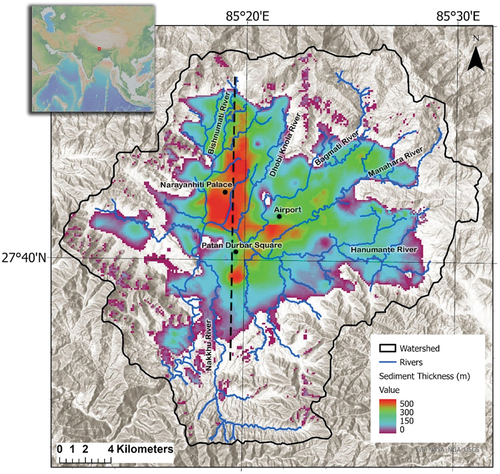
The Kathmandu Basin lies within the Kathmandu Nappe, which consists of Precambrian crystalline rocks and Precambrian-Ordovician sedimentary rocks, forming the basement and surrounding hills of the Kathmandu basin (Figure 2) (DMG 2011; Stöcklin and Bhattarai 1977). However, the Pliocene-Pleistocene unconsolidated basin-fill sediment unconformably overlies the eroded surface of the Precambrian basement rocks (Sakai et al. 2006). The spatial distribution of the basin-fill sediment is not homogeneous as it consists of sandy layers in the northern part, silty-clay in the central part and sandy-gravel layers in the southern part of the basin (Sakai et al. 2012). The greatest thickness of the sediment is ~500 m in the central part of the basin. Exposed isolated basement rocks within the basin along with geophysical investigations and drill core results indicate that the sediment thickness is not uniform and that the basal unconformity is irregular (Moribayashi and Maruo 1980; Paudyal et al. 2013).

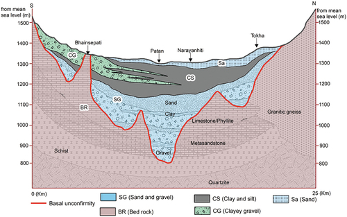
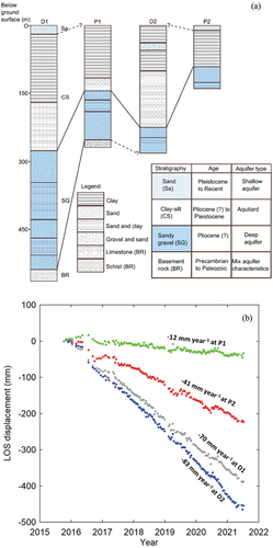
Figure 2. North-South generalized representative cross-section schematic model of Kathmandu Valley. An approximate location of the cross-section is shown in Figure 1 as a black dashed line. The basin stratigraphy is classified into five distinct stratigraphic units. Sa represents the shallow aquifer, SG represents the deep aquifer, CS represents the aquitard and CG with mixed aquifer characteristics. BR is the basement made up of metasandstone, phyllite, schist and quartzite. The maximum thickness of the aquitard is ~200 m and similarly the maximum thickness of the deep aquifer is ~300 m around the central part of the basin. The central part of the basin is the region where the maximum subsidence is observed. The shallow aquifer is recharged during each monsoon season directly from the precipitation. The chances of vertical recharge for the deep aquifer from precipitation is negligible due to the presence of a thick aquitard above it. Infiltration from the top sandy layer and bed rock aquifer (weathered gneiss, metasandstone, limestone) in the marginal part may have some contribution to the deep aquifer. Note that the maximum variation in thickness is controlled by the lower sandy gravel unit (SG), which represents the deep aquifer.

Kathmandu city has a population density of ~20,000 people per square km (https://worldpopulationreview.com/countries/nepal-population), as of 2013, is the fastest growing metropolitan area in South Asia (Muzzini and Aparicio 2013). The urban area in Kathmandu has expanded over 400% with a ~>30% loss of agricultural land, the majority of this expansion happened between 1989 and 2009 (Ishtiaque, Shrestha, and Chhetri 2017). Nearly half of the total water supply during the wet season and almost 70% during the dry season is sourced from sub-surface water (ICIMOD 2007). Groundwater extraction in the basin started in the 1980s and the rate of extraction has increased since then (Pandey, Shrestha, and Kazama 2012). Both shallow and deep aquifers are being used for groundwater extraction. The Pliocene deep aquifer, dominantly fluvial sandy-gravel, is overlain by a thick lacustrine silty-clay aquitard and capped by a shallow gravelly upper aquifer succession (Sakai et al. 2006, 2012). However, the lateral and vertical distribution of aquifer and aquitard is poorly known.

The consequences of rapid urbanization are already seen in the form of changes in the surface runoff of water, recharge dynamics of groundwater and the decreasing volumes of water in the basin (Dong and Karmacharya 2018; Gupte and Bogati 2014; Mesta, Cremen, and Galasso 2022). The projected changes are expected to escalate the depletion of sub-surface water levels with further changes expected in the base flows in rivers (Lamichhane and Shakya 2019). The estimated thickness of the shallow aquifer varies from 0 to 85 m, with the corresponding aquitard thickness varying from less than 5 m to more than 200 m, and the deep aquifer thicknesses varying from 25 m to more than 285 m (Pandey, Shrestha, and Kazama 2012). However, there is inconsistency in how the aquifers are classified based on depth, posing challenges to their management (Gurung et al. 2007; Khadka 1993). Most importantly, there is no significant vertical recharge to the deep aquifers which are confined aquifers overlain by thick aquitards (Gurung et al. 2007; Shakya et al. 2019). There is some limited recharge area in the northern margin of basin, where the deep aquifer is connected with the shallow aquifer (Pandey, Chapagain, and Kazama 2010). The shallow aquifers are generally represented by the top sandy layers that are recharged during the monsoon season (Gurung et al. 2007). Hence, the Kathmandu groundwater system consists of unconfined, mainly shallow aquifers, confined deep aquifers overlain by a thick aquitards and partially rechargeable aquifers in the marginal parts of the basin where the sediment and/or aquitard thickness is thinner.

Land subsidence is a common problem in rapidly urbanizing areas due to aquifer depletion (Herrera-García et al. 2021; Khan et al. 2023). For example, due to groundwater exploitation and the slow drainage of clay aquitards, Mexico City currently has a subsidence rate of up to 390 mm year⁻¹ which is causing permanent irreversible compaction (Cigna and Tapete 2021). Groundwater-exploitation-related problems have also been observed in Delhi, which had subsidence rates of up to 60 mm year⁻¹ from 2014 to 2019 (Kumar et al. 2022), and Jakarta that had subsidence rates up to 280 mm year⁻¹ from 1982 to 2010 (Abidin et al. 2011). The unsustainable use of groundwater resources creates problems, with increasing risk of flood exposure (Cigna and Tapete 2021) as well as surface-deformation-induced structural damage (Huang et al. 2016).

Kathmandu is a rapidly subsiding city, the average subsidence rate around the Narayanhiti Palace in Kathmandu was 80 mm year⁻¹ between 2007 and 2011, and increased to 150 mm year⁻¹ during early post 2015 Gorkha earthquake. This short-lived subsidence rate increase lasted around 3 months, then returned back to the long-term subsidence rate of 120 mm year⁻¹ at the end of 2015 (Suresh-Krishnan, Kim, and Jung 2018). The high subsidence rates are a significant concern for cities like Kathmandu, where rapid population growth presents a risk to future sustainable development.

To address the issue of subsidence in Kathmandu, this study applies multi-temporal InSAR observations to analyse the present-day surface subsidence rates. The spatial distribution of subsidence is compared to sediment thicknesses and to the modern river network. Annual rainfall variations are also considered in terms of evidence of seasonal responses to monsoon precipitation. The data demonstrate the degree of variability and the ongoing high rates of subsidence across the metropolitan city and consider the probable role of water extraction.

2. InSAR methodology

InSAR (Interferometric Synthetic Aperture Radar) is used to measure ground deformation, such as subsidence, across extensive areas. SBAS-InSAR (Small Baseline Subset Interferometric Synthetic Aperture Radar) is a stacking InSAR technique that works by combining InSAR images from the same area taken at different times and using the phase differences between the images to calculate the change in the distance between the satellite radar sensor and the ground (Bürgmann, Rosen, and Fielding 2000; Massonnet and Feigl 1998). The InSAR results are then used to generate maps of ground deformation and to track changes in the ground deformation over a specified time. InSAR data provide valuable information about the extent and severity of subsidence in any given landmass (Tomás et al. 2005, 2014). SBAS-InSAR is an established processing technique used to process InSAR images for monitoring millimetre-scale surface deformation around the world.

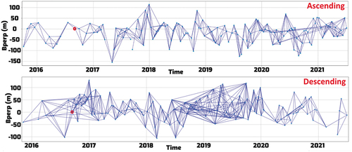
The input SAR interferograms are 450 ascending and 286 descending C-band images from Sentinel-1 A/B satellites during 2015–2021 (ascending frame 2015/10/06–2021/07/06 and descending frame 2015/11/07–2021/07/02). This time series excludes the ~100-day period of post-seismic high subsidence due to sediment oscillation, from the 2015 Gorkha earthquake (Suresh-Krishnan, Kim, and Jung 2018). The frame number for the ascending frame is 085A_06253_131313 and for the descending frame is 019D_06217_131313. The Sentinel-1 A/B SAR images footprint size is 250 × 250 km, with a 6-day revisit time. The SAR interferogram data were processed by the COMET LiCSAR system (Lazecký et al. 2020), which uses GAMMA software. Data are available from the LiCSAR portal (https://comet.nerc.ac.uk/comet-lics-portal/).

During processing, we chose to clip the SAR footprint to an area that covers only the Kathmandu Valley watershed. To observe the recent surface movement velocity and time-series in the valley, we used the LiCSBAS package (Morishita et al. 2020), which applied the SBAS technique to the SAR interferogram images downloaded from LiCSAR system. LiCSBAS is an open-source software written in Python3 and uses small baseline (SB) inversion to produce surface movement velocity maps at 100 × 100-m spatial resolution with accuracies on the order of ~2 mm year⁻¹. A network of the available interferometric pairs and baseline information is shown in Figure 3. The interferograms are combined to derive the surface deformation velocities by inversion of the temporal phase profiles, effectively reducing atmospheric noise, and topographic effects. The GACOS (Generic Atmospheric Correction Online Service) atmospheric correction is also applied to both the ascending and descending frames during processing (Yu et al. 2018; Yu, Li, and Penna 2018; Yu, Penna, and Li 2017).

Figure 3. The network of all available pairs of interferograms. The y-axis is the perpendicular baseline, versus acquisition dates on the x-axis. The perpendicular baseline is the distance between the satellite orbits when the satellite revisits the ‘same location’. Each blue line connects two SAR images for interferograms. All the SAR images are co-registered with the master reference SAR image (red circle, 2016/09/14 for the descending and 2016/09/06 for the ascending).

We use the LiCSBAS auto-selected reference point (black star, Figure 4a), which is based on high coherence away from rapidly subsiding regions. The line-of-sight velocity results from both the ascending and descending frames are analogous (Figure 4). The ascending and descending results were combined to decompose the LOS direction motion to vertical and horizontal motion by using LiCSBAS software (Morishita et al. 2020). There is an assumption that there is no North–South displacement due to the SAR satellite having near polar orbits that are insensitive to North–South motion. So, the horizontal motion in Figure 4d is in the East–West direction. To estimate the uncertainty of the SBAS-InSAR LOS velocity, the standard deviation is calculated based on the bootstrap method using the LiCSBAS software (Morishita et al. 2020). The SBAS-InSAR results from both ascending and descending results have an accuracy of ~1 mm year⁻¹ (Figure 5).

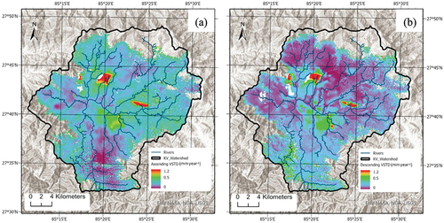
Figure 4. The SBAS-InSAR results from (a) 2015/10/06 to 2021/07/06 for the ascending and (b) 2015/11/07 to 2021/07/02 for the descending. The overall velocities from the ascending and descending are similar. (c) The vertical velocities are from 2015/11/07 to 2021/07/02. (d) In the horizontal (EW) motion map, positive values mean eastward displacement. The 10 coloured triangles in (a) are the locations for the time-series analysis. The reference point in (a) is the black star located in the south of the Kathmandu Valley. The yellow square in (a) is the GPS location.

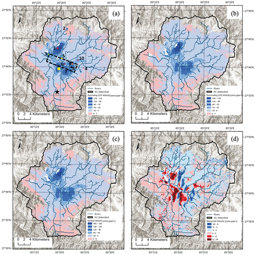
Figure 5. Maps of uncertainty in the subsidence rates. (a) Ascending velocity standard deviation. (b) descending velocity standard deviation. InSAR LOS velocity standard deviation ranges 0–1 mm year⁻¹. The relative high values in velocity standard deviation could be caused by relatively high uncertainty values, or a non-linear signal in the time-series.

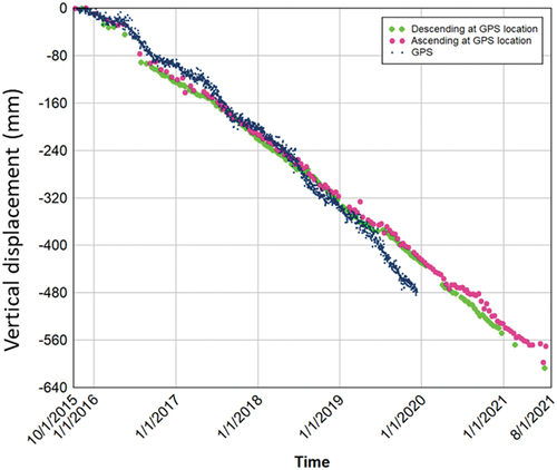
Sentinel-1 deformation records were compared with GPS data. There are two continuously operating GPS stations (KKN4 and NAST) available from the UNAVCO website. We choose the NAST GPS station to compare with the InSAR results, due to its best data quality. The NAST location is marked with a yellow square in Figure 4a. The GPS data are processed by the Nevada Geodetic Laboratory (NGL) from the University of Nevada (Blewitt and Hammond 2018). The GPS station’s position is determined on its own, without reference or use of nearby stations (http://geodesy.unr.edu/NGLStationPages/stations/NAST.sta). The ascending and descending SBAS-InSAR time series from the same location as the NAST GPS are shown in Figure 6. To be able to compare with the GPS vertical velocity, we converted those line-of-sight velocity values to vertical velocity values based on the following equation, which assumes that all observed deformations are vertical.

${\mathrm{V}}_{\mathrm{vertical}}={\mathrm{V}}_{\mathrm{LOS}}/cos{38.8}^{\circ }$

Figure 6. Comparison of the GPS, ascending and descending SBAS-InSAR time-series at the NAST-GPS location. The InSAR derived time-series at the GPS location closely agrees with the time series measured by GPS. The NGL has GPS data available up to year 2020 at this GPS location. There is a small acceleration of the subsidence rate picked up by the GPS in year 2019, however this change is not resolved in the InSAR result. This could be explained by the spatial resolution difference between those two techniques.

where 38.8° is the Sentinel-1 satellite SAR acquisition average incident angle.

While the vertical movement time-series trends from both InSAR and GPS are similar, the subsidence rates are different. The vertical velocity for SBAS-InSAR is −105 mm year⁻¹ (2015–2021) (Figure 6), and the GPS vertical velocity is −112 mm year⁻¹ (2015–2020). This variation may arise from differences in the measurement direction, temporal span, spatial resolution and reference points.

3. Results

3.1. Spatial distribution of surface deformation

According to the six-year (2015–2021) Sentinel-1 A/B results, the majority of the Kathmandu Valley that is filled by sediment is subsiding (Figure 7). The InSAR LOS velocity values from the ascending results are in the range of −170 to +36 mm year⁻¹, and the descending results are in the range of −165 to +21 mm year⁻¹. The vertical velocity results are in the range of −205 to +18 mm year⁻¹, and the horizontal velocity results are in the range of −28 to +36 mm year⁻¹ (Figure S1). The value distribution histograms only have a few outliers with extremely high positive values in the ascending, descending and vertical velocity results, and are located at the edge of the Kathmandu Valley. In order to ensure a consistent dataset, a few outliers with high positive values in the ascending, descending and vertical results, which are likely caused by the high topography and low coherence effect at the edge of the valley, are removed. The extreme negative values in the ascending, descending, vertical and both the extreme positive and negative values in the horizontal velocity results are all located at the middle of the valley with high coherence, and those values are kept (Figure 4). The dominant vertical rate is in the range of −60 to 8 mm year⁻¹ (Figure S1), and the centre of maximum subsidence (marked by a red contour line in Figure 7a) has a vertical subsidence rate of up to ~200 mm year⁻¹. The localized subsidence is accompanied by E-W compression with a range of ~ ±30 mm year⁻¹ (Figure 4d). The subsidence motion points to the centre of each subsiding zone (Cigna and Tapete 2021). There is no subsidence in areas with exposed bedrock (no sediment), and in fact, these areas have an uplift rate in the range of 0–5 mm year⁻¹ (Figure 7a). The uplift ground motion is driven by the well-documented background regional tectonics (Ader et al. 2012).

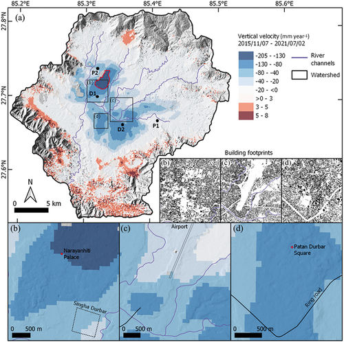
Figure 7. (a) Spatial distribution of the SBAS-InSAR surface vertical deformation result in relation to the main urban landmarks: (b) Narayanhiti Palace, (c) airport, (d) Patan Durbar Square. Building footprints are shown from Microsoft’s GlobalMLBuildingFootprints dataset (https://github.com/microsoft/GlobalMLBuildingFootprints). The four black dots in (a) are the locations of the four deep water wells used in stratigraphic column analysis.

Bivariate analysis of the InSAR vertical velocity and sediment thickness within the watershed (Figure 8) indicates a positive correlation between subsidence rates and sediment thickness. The most rapid subsidence rates occur in the area with a sediment thickness of ~400 m (marked by red contour in Figure 7a and red coloured point cloud in Figure 8a). The crossplot shows the lithological spatial distribution of the response to water withdrawal in different lithologies. Maximum subsidence rates could be due to compaction in sediment with a high clay content (Figure 2). A detailed distribution of the density of the points is most likely controlled by lithological heterogeneity in the underlying sedimentary succession. The densest points located around −10 mm year⁻¹ are probably from a sandy layer in the sediment, which shows a positive linear correlation between sediment thickness and subsidence rate. The middle part of the point cloud with subsidence rates from −30 to −130 mm year⁻¹ probably results from a clay mixture sediment (Clayey Gravel in Figure 2). The four black dots in Figure 7a indicate the deep well locations used for the stratigraphic column (Figure 9a). The stratigraphic column at those four available locations shows an example of the correlation between subsidence rates and sediment thickness (Figure 8a). The information from the stratigraphic columns indicates a complex relationship between the deep aquifer thickness and the subsidence rate. This could indicate that the subsidence rate is a function of both the shallow and deep aquifers and that the heterogeneous nature of the stratigraphy (Figure 2) generates complex groundwater conditions.

Figure 8. (a) InSAR vertical velocity and sediment thickness crossplot within the entire watershed area. Each dot represents a pixel value of 130 × 130 m in size. There is a basic positive correlation of increased sediment thickness with increasing vertical subsidence velocity around −10 mm year⁻¹. A cluster of high subsidence rate points (<-130 mm year⁻¹) is located near Narayanhiti Palace (the red contour area in Figure 7). (b) The InSAR vertical velocity and DTM crossplot within the entire watershed area. Each dot represents a pixel value of 130 × 130 m. The red vertical line at the zero point differentiates those points uplifting and subsiding.

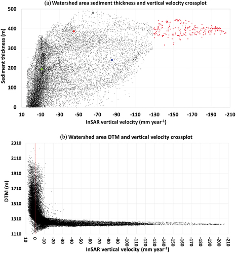
Figure 9. (a) Stratigraphy column from four deep water wells across the basin shows shallow and deep aquifers. This figure illustrates the representative stratigraphic columns of the Kathmandu basin, based on the lithological logs obtained from deep wells. The locations of these wells are indicated on the map (see Figure 7). The basin-fill sediments are categorized into three stratigraphic units. The ‘SG’ unit predominantly consists of sand and gravel layers, indicative of paleo-fluvial and early lacustrine deposits. These units, including the top weathering surface of the bedrock (‘BR’), exhibit favourable aquifer characteristics and serve as a significant water source for deep water tube wells in the basin. The ‘Cs’ unit is primarily comprised of clay and silt, interspersed with sandy lenses. It predominantly represents lacustrine sediments that deposited during periods where water ponded in the basin. The thickness of this unit varies from a few metres to approximately 300 metres. The sandy lenses and silt layers within this unit also serve as water sources for water wells in the basin. The top ‘Sa’ represents a mainly sandy sequence deposited after the basin drainage. It serves as a suitable aquifer for shallow wells, receiving recharge during the rainy season (data source: (DMG 1988; Pandey et al. 2023)). (b) Four deep water well locations have been analysed using InSAR time-series to show their LOS subsidence rates. In Figure 8a, locations of well P1, P2 and D1 show a clear linear correlation between vertical velocity and sediment thickness, while D2 deviates from this trend. Figure 9a illustrates how the ambiguous boundaries of D2’s shallow and deep aquifers in the stratigraphic column might account for this uncertainty.

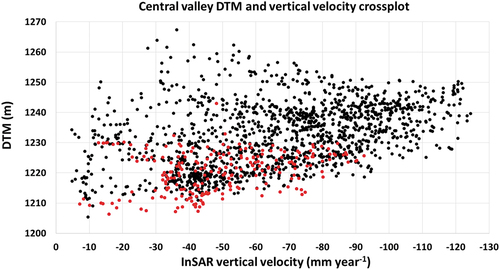
To further investigate these patterns, we focus on an area where the elevation of the river channels is relatively stable and compare it with the subsidence rates of the surrounding floodplains. We select an area from the centre of the Kathmandu Valley where the elevation of the river channels is relatively stable (black dotted polygon in Figure 4a) for DTM (Digital Terrain Models) and InSAR vertical velocity crossplot (Figure 10). The result shows the average vertical subsidence rate at the river channels is −60 mm year⁻¹; however, the floodplain has an average subsidence rate of −80 mm year⁻¹. There is a high differential subsidence gradient (20 mm year⁻¹) between the river channel and its surrounding areas.

Figure 10. InSAR vertical velocity and DTM crossplot. Each dot represents a pixel size of 130 × 130 m. The red dots show the points that are along the river channel that cover a 130 m area, due to the pixel size. Within a small sample area around the Kathmandu Valley’s central rivers (indicated by the black dotted polygon in Figure 4a), linear trends show increasing vertical velocities with rising elevation. The lower values along the river channels are likely associated with recharging from the river to its immediate surroundings.

3.2. Linear and sinusoidal signal patterns in the time-series

We chose 10 different locations (triangles in Figure 4a) that characterize the typical signal pattern of the time-series (Figure 11a). The time-series pattern shows the character of surface movement behaviour at a given location. Location 1 is in the centre of the Kathmandu metropolitan region and has the most rapid subsidence rate (line-of-sight velocity −160 mm year⁻¹). Location 2 is in an area of exposed bedrock in the mountains in the north with ~3 mm year⁻¹ uplift rate. The time-series from locations 1, 3, 5–10, centred in distinct subsidence zones, show a similar trend of long-term linear subsidence (Figure 11a). The seasonal sinusoidal annual variation may be masked by the high subsidence rates at those locations, or be a signal of deep aquifer-related subsidence with no annual recharge.

Figure 11. (a) Time-series from the ascending frame at 10 different locations indicated in triangles in Figure 4a. (b) Averaged time-series at location 4 from both the ascending and descending frames. The annual sinusoidal signal is marked by red dotted lines that peak in the month of July. Because the raw result from the SBAS-InSAR is velocity from the line-of-sight direction, the time-series plots the changes of accumulated line-of-sight displacement with time.

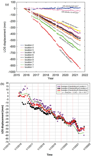
Location 4 is located near the Hanumante River, which has a −12 mm year⁻¹ subsidence rate, and an annual sinusoidal pattern. To confirm this potential annual sinusoidal pattern, we average four adjacent pixels at location 4, and compare both the ascending and descending time-series to elucidate the sinusoids (Figure 11b). Based on both the ascending and descending signals, a convincing annual sinusoidal peak occurs around the middle of the year (~July) and is marked by red dotted lines in Figure 11b. To pick the sinusoidal peak objectively based on the character of the seasonal signal, we fit a sinusoidal curve to the observed time-series at location 4 that averages both the ascending and descending results (Figure 11b). This fitted sinusoidal signal has an assumed annual variation. For other parameters, such as amplitude, phase and slope, we choose the value that brings the lowest standard deviation to the curve fit.

4. Discussion

The InSAR-mapped subsidence corresponds to regions in the Kathmandu Valley with thicker Pliocene to recent sediment deposits (Figure 1). A broadly positive correlation between sediment thickness and subsidence rate suggests that the dominant driver of subsidence in this region is not tectonic but is related to the underlying sedimentary succession (Figure 8). The broad scatter for large portions of the data in Figure 8(a) is most easily explained by the distribution of different lithologies and hence hydraulic properties in the Pliocene to Recent succession (Figure 2 and 9). The sediment in the valley contains shallow aquifers, clay aquitards and deep aquifers. The sediment compaction mechanisms could be natural compaction of sediment, compaction due to infrastructure and housing development or compaction resulting from water extraction. Given that the youngest age of the sediment is ca. 35,000 yrs old, then a rate of 200 mm year⁻¹ would equate to 700 m of subsidence since deposition of the sediment; this is physically unreasonable if it were simply post-depositional compaction, and so other mechanisms are needed. We see no evidence of a correlation between density of buildings and subsidence as would be expected if urban development had determined the signal (Figure 7b–d). The simplest interpretation is that the ongoing subsidence is generated by water extraction as witnessed in other regions such as Mexico City (Cigna and Tapete 2021). The shallow aquifer groundwater level from the years 2000–2019 shows no correlation with the InSAR ground subsidence rate (Figure S2). The sediment thickness in the deep aquifer is more variable than the aquitard and shallow aquifer thicknesses as it fills in an irregular basal unconformity; this variable thickness in the deep aquifer is therefore the primary control for the variation in the total sediment thickness (Figure 2 and 8). This suggests that the thick pile of sandy gravel beneath the clay-silt aquitard is the deep aquifer from which the bulk of the water has been extracted, causing a tight link between sediment thickness and surface subsidence.

The majority of the signal in the time-series is a strong linear subsidence signal in the Kathmandu Valley. The time-series that centred in different subsidence zones all show a similar signal of long-term linear subsidence with any slight variations from the long-term trend mimicked in each of the zones. This similarity in the subsidence signal between zones suggests that the deep aquifer is hydrologically connected, and so the deep aquifer system behaves with a uniform signal, but varying magnitude (Figure 11a). The areas with relative low subsidence rate (~10 mm year⁻¹), with possible dominant water extraction from shallow aquifers, show stronger sinusoidal annual variation peaks in July during the monsoon season (Figure 11b). The sinusoidal signal is likely from the influence of a shallow aquifer, with changes caused by seasonal rainfall, which leads to hydraulic head variances in the surface sediment. Decreases in hydraulic head cause groundwater outflow, and the result is subsidence. Increases in hydraulic head cause groundwater inflow, and result in uplift. The sinusoidal signal reaches annual maxima amplitude around July which is within the June–August monsoon season.

Further detailed hydrology studies with integration of InSAR, subsurface lithology and DTM are needed. Better documentation of water withdrawal rates from both shallow and particularly deep aquifers could provide a better understanding of the compaction at depth. Pandey et al. (2010) suggest that less than half of the groundwater extraction from the deep aquifer has been recharged annually from the northern margin of the valley, and our study supports this. Based on built-up urban areas from 2002 (Marconcini et al. 2021) and 2020 (Zanaga et al. 2022), the city has significantly expanded to the north margin of the valley since 2002 (Figure S3). Reduced natural recharge and unlicensed groundwater exploitation will likely result in the subsidence issues continuing, potentially leading to irreversible permanent deformation in the deep aquifer's hydrological properties. Similarly, irreversible permanent deformation in a deep confined aquifer has been documented in the Central Valley in California (Faunt et al. 2016).

A clear correlation exists between low subsidence rates and low DTM elevations around the valley’s central river channel (Figure 10), indicating possible recharge of the surface aquifer groundwater from the river. Bajracharya et al. (2018) use electrical conductivity measurements of shallow water wells along the major Kathmandu rivers, to show the possibility of polluted river water recharging a shallow aquifer up to 60 m away from river channels. Kathmandu Public Health also reported that solid waste disposal into rivers has caused water-borne diseases that have been the cause of the high percentage of deaths in local areas (Pandey, Chapagain, and Kazama 2010).

The high differential subsidence gradient at the river channel and its surrounding areas increases exposure to flood risk. For example, at the Hanumante river channel and its river bank area, the vertical subsidence rate difference is ~60 mm year⁻¹. The elevation difference between the Manahara river bank and its river channel floor is ~20 m, which is predicted to vanish in the next 300 years. Historical architectural centres such as the Singha Durbar, Narayanhiti Palace and Patan Durbar Square (Figure 7b–d) situated near these river channels in the valley, now face increased flood risk.

5. Conclusion

In this study, we analyse spatial and temporal records of ground subsidence in the Kathmandu Valley using Sentinel-1 InSAR observations (2015–2021). Subsidence distribution and rates across the Kathmandu Valley show remarkably rapid subsidence rates in the centre of the valley (up to 200 mm year⁻¹). In the Kathmandu Valley subsidence is primarily controlled by the thickness of the underlying sedimentary succession, evidenced by the positive correlation between sediment thickness and subsidence rate. The deep aquifer groundwater extraction is likely to be the first-order control on the variable compaction response. However, internal heterogeneity of the sediment packages also contributes to the sediment compaction variation. Ground deformation time-series reveal a strong linear subsidence signal, further accentuated by the deep aquifer’s hydrological connection. River recharge caused differential subsidence gradient could potentially increase vulnerability and exposure to flood risk within the valley.

Highlights

• InSAR shows up to 200 mm year-1 subsidence rate since 2015 in the Kathmandu Valley.

• Deep aquifer compaction is the main driver of subsidence.

• Time-series show dominant linear subsidence signal, with weak sinusoidal peaks related to seasonal aquifer recharge.

• High subsidence gradients around rivers affect flood risk.

Acknowledgements

We thank Yu Morishita for great technical support during the InSAR data processing. We thank John Elliott, Maggie Creed, Christopher McDermott and Lei Sun for helpful discussions. We thank the European Space Agency (ESA), Centre for the Observation and Modelling of Earthquakes, Volcanoes and Tectonics (COMET) lab, Nevada Geodetic Laboratory (NGL). JH is supported by a Daphne Jackson Fellowship, funded by Natural Environment Research Council (NERC). CSW is funded by the UK Research and Innovation (UKRI) Global Challenges Research Fund (GCRF) Urban Disaster Risk Hub (NE/S009000/1) (Tomorrow’s Cities) and COMET.

Disclosure statement

No potential conflict of interest was reported by the author(s).

Supplemental data

Supplemental data for this article can be accessed online at https://doi.org/10.1080/01431161.2023.2283902.

Additional information

Funding

The work was supported by the Natural Environment Research Council; UK Research and Innovation Global Challenges Research Fund [NE/S009000/1].

References

- Abidin, H. Z., H. Andreas, I. Gumilar, Y. Fukuda, Y. E. Pohan, and T. Deguchi. 2011. “Land Subsidence of Jakarta (Indonesia) and Its Relation with Urban Development.” Natural Hazards 59 (3): 1753–1771. https://doi.org/10.1007/s11069-011-9866-9.
- Ader, T., J. P. Avouac, J. Liu‐Zeng, H. Lyon‐Caen, L. Bollinger, J. Galetzka, J. Genrich, M. Thomas, K. Chanard, and S. N. Sapkota. 2012. “Convergence Rate Across the Nepal Himalaya and Interseismic Coupling on the Main Himalayan Thrust: Implications for Seismic Hazard.” Journal of Geophysical Research: Solid Earth 117 (B4). https://doi.org/10.1029/2011JB009071.
- Avouac, J.-P. 2015. “From Geodetic Imaging of Seismic and Aseismic Fault Slip to Dynamic Modeling of the Seismic Cycle.” Annual Review of Earth and Planetary Sciences 43 (1): 233–271. https://doi.org/10.1146/annurev-earth-060614-105302.
- Bajracharya, R., N. K. Tamrakar, M. Shrestha, and B. Bohara. 2018. “Status of Shallow Wells Along Major Rivers of the Kathmandu Valley, Central Nepal.” Journal of Nepal Geological Society 56 (1): 31–42. https://doi.org/10.3126/jngs.v56i1.22697.
- Bhattarai, R., H. Alifu, A. Maitiniyazi, and A. Kondoh. 2017. “Detection of land subsidence in Kathmandu Valley, Nepal, using DInSAR technique.” Land 6 (2): 39. https://doi.org/10.3390/land6020039.
- Bilham, R. 2019. “Himalayan Earthquakes: A Review of Historical Seismicity and Early 21st Century Slip Potential.” Geological Society, London, Special Publications 483 (1): 423–482. https://doi.org/10.1144/SP483.16.
- Blewitt, G., and W. Hammond. 2018. “Harnessing the GPS Data Explosion for Interdisciplinary Science.” Eos 99. https://doi.org/10.1029/2018EO104623.
- Bürgmann, R., P. A. Rosen, and E. J. Fielding. 2000. “Synthetic Aperture Radar Interferometry to Measure Earth’s Surface Topography and Its Deformation.” Annual Review of Earth and Planetary Sciences 28 (1): 169–209. https://doi.org/10.1146/annurev.earth.28.1.169.
- Chen, W. P., and P. Molnar. 1977. “Seismic Moments of Major Earthquakes and the Average Rate of Slip in Central Asia.” Journal of Geophysical Research 82 (20): 2945–2969. https://doi.org/10.1029/JB082i020p02945.
- Cigna, F., and D. Tapete. 2021. “Present-Day Land Subsidence Rates, Surface Faulting Hazard and Risk in Mexico City with 2014–2020 Sentinel-1 IW InSar.” Remote Sensing of Environment 253:112161. https://doi.org/10.1016/j.rse.2020.112161.
- DMG. 1988. Kathmandu Gas Well Construction, Gas Project Report, Nepal. In D.o.M.a. Geology (Ed.)
- DMG. 2011. Geological Map of Central Nepal. In. Department of Mines and Geology (DMG)
- Dong, P. J., and T. Karmacharya. 2018. “Impact of Urbanization on Public Health in Kathmandu Valley, Nepal-A Review.” Juniper Online Journal of Public Health 3 (4): 001–0011. https://doi.org/10.19080/JOJPH.2018.03.555617.
- Elliott, J., R. Jolivet, P. J. González, J.-P. Avouac, J. Hollingsworth, M. Searle, and V. Stevens. 2016. “Himalayan Megathrust Geometry and Relation to Topography Revealed by the Gorkha Earthquake.” Nature Geoscience 9 (2): 174–180. https://doi.org/10.1038/ngeo2623.
- Faunt, C. C., M. Sneed, J. Traum, and J. T. Brandt. 2016. “Avaliação hídrica e subsidência de terreno no Vale Central, Califórnia, EUA.” Hydrogeology Journal 24 (3): 675–684. https://doi.org/10.1007/s10040-015-1339-x.
- Gupte, J., and S. Bogati. 2014. Key Challenges of Security Provision in Rapidly Urbanising Contexts: Evidence from Kathmandu Valley and Terai Regions of Nepal. In. No. IDS Evidence Report; 69.
- Gurung, J. K., H. Ishiga, M. S. Khadka, and N. R. Shrestha. 2007. “The Geochemical Study of Fluvio-Lacustrine Aquifers in the Kathmandu Basin (Nepal) and the Implications for the Mobilization of Arsenic.” Environmental Geology 52 (3): 503–517. https://doi.org/10.1007/s00254-006-0483-y.
- Herrera-García, G., P. Ezquerro, R. Tomás, M. Béjar-Pizarro, J. López-Vinielles, M. Rossi, R. M. Mateos, D. Carreón-Freyre, J. Lambert, and P. Teatini. 2021. “Mapping the Global Threat of Land Subsidence.” Science 371 (6524): 34–36. https://doi.org/10.1126/science.abb8549.
- Huang, J., S. D. Khan, A. Ghulam, W. Crupa, I. A. Abir, A. S. Khan, D. M. Kakar, A. Kasi, and N. Kakar. 2016. “Study of Subsidence and Earthquake Swarms in the Western Pakistan.” Remote Sensing 8 (11): 956. https://doi.org/10.3390/rs8110956.
- ICIMOD. 2007. Kathmandu Valley Environmental Outlook. Kathmandu: Hillside Press (P.) Ltd.
- Ingleby, T., T. Wright, A. Hooper, T. Craig, and J. Elliott. 2020. “Constraints on the Geometry and Frictional Properties of the Main Himalayan Thrust Using Coseismic, Postseismic, and Interseismic Deformation in Nepal.” Journal of Geophysical Research: Solid Earth 125 (2): e2019JB019201. https://doi.org/10.1029/2019JB019201.
- Ishtiaque, A., M. Shrestha, and N. Chhetri. 2017. “Rapid Urban Growth in the Kathmandu Valley, Nepal: Monitoring Land Use Land Cover Dynamics of a Himalayan City with Landsat Imageries.” Environments 4 (4): 72. https://doi.org/10.3390/environments4040072.
- JICA. 2018. The Project for Assessment of Earthquake Disaster Risk for the Kathmandu Valley in Nepal. In. Japan International Cooperation Agency
- Khadka, M. S. 1993. “The Groundwater Quality Situation in Alluvial Aquifers of the Kathmandu Valley, Nepal.” AGSO Journal of Australian Geology & Geophysics 14 (2/3): 207–211.
- Khan, S. D., M. I. Faiz, O. C. Gadea, and L. Ahmad. 2023. “Study of Land Subsidence by Radar Interferometry and Hot Spot Analysis Techniques in the Peshawar Basin, Pakistan.” The Egyptian Journal of Remote Sensing & Space Science 26 (1): 173–184. https://doi.org/10.1016/j.ejrs.2023.02.001.
- Kumar, H., T. H. Syed, F. Amelung, R. Agrawal, and A. Venkatesh. 2022. “Space-Time Evolution of Land Subsidence in the National Capital Region of India Using ALOS-1 and Sentinel-1 SAR Data: Evidence for Groundwater Overexploitation.” Canadian Journal of Fisheries and Aquatic Sciences 605:127329. https://doi.org/10.1016/j.jhydrol.2021.127329.
- Lamichhane, S., and N. M. Shakya. 2019. “Alteration of Groundwater Recharge Areas Due to Land Use/Cover Change in Kathmandu Valley, Nepal.” Journal of Hydrology: Regional Studies 26:100635. https://doi.org/10.1016/j.ejrh.2019.100635.
- Lazecký, M., K. Spaans, P. J. González, Y. Maghsoudi, Y. Morishita, F. Albino, J. Elliott, N. Greenall, E. Hatton, and A. Hooper. 2020. “LiCsar: An Automatic InSar Tool for Measuring and Monitoring Tectonic and Volcanic Activity.” Remote Sensing 12 (15): 2430. https://doi.org/10.3390/rs12152430.
- Marconcini, M., A. Metz-Marconcini, T. Esch, and N. Gorelick. 2021. “Understanding Current Trends in Global Urbanisation-The World Settlement Footprint Suite.” GI_Forum 9: 33–38.
- Massonnet, D., and K. L. Feigl. 1998. “Radar Interferometry and Its Application to Changes in the Earth’s Surface.” Reviews of Geophysics 36:441–500. https://doi.org/10.1029/97RG03139.
- Mesta, C., G. Cremen, and C. Galasso. 2022. “Urban Growth Modelling and Social Vulnerability Assessment for a Hazardous Kathmandu Valley.” Scientific Reports 12 (1): 6152. https://doi.org/10.1038/s41598-022-09347-x.
- Moribayashi, S., and Y. Maruo. 1980. “Basement Topography of the Kathmandu Valley, Nepal - an Application of Gravitational Method to the Survey of a Tectonic Basin in the Himalayas.” Journal of the Japan Society of Engineering Geology 21 (2): 80–87. https://doi.org/10.5110/jjseg.21.80.
- Morishita, Y., M. Lazecky, T. J. Wright, J. R. Weiss, J. R. Elliott, and A. Hooper. 2020. “LiCsbas: An Open-Source InSar Time Series Analysis Package Integrated with the LiCsar Automated Sentinel-1 InSar Processor.” Remote Sensing 12 (3): 424. https://doi.org/10.3390/rs12030424.
- Muzzini, E., and G. Aparicio. 2013. Urban Growth and Spatial Transition in Nepal: An Initial Assessment. Washington, D.C., United States: World Bank Publications.
- Pandey, V. P., S. K. Chapagain, and F. Kazama. 2010. “Evaluation of Groundwater Environment of Kathmandu Valley.” Environmental Earth Sciences 60 (6): 1329–1342. https://doi.org/10.1007/s12665-009-0263-6.
- Pandey, V. P., S. B. Rana, S. D. Shrestha, and A. Khanal. 2023. Groundwater in Kathmandu Valley: Status, Challenges and Opportunities. In N. Kathmandu Valley Water Supply Management Board (KVWSMB) (Ed.)
- Pandey, V., S. Shrestha, and F. Kazama. 2012. “Groundwater in the Kathmandu Valley: Development Dynamics, Consequences and Prospects for Sustainable Management.” European Water 37 (2012): 3–14.
- Paudyal, Y. R., R. Yatabe, N. P. Bhandary, and R. K. Dahal. 2013. “Basement Topography of the Kathmandu Basin Using Microtremor Observation.” Journal of Asian Earth Sciences 62:627–637. https://doi.org/10.1016/j.jseaes.2012.11.011.
- Ryan, W. B., S. M. Carbotte, J. O. Coplan, S. O’Hara, A. Melkonian, R. Arko, R. A. Weissel, V. Ferrini, A. Goodwillie, and F. Nitsche. 2009. “Global Multi‐Resolution Topography Synthesis.” Geochemistry, Geophysics, Geosystems 10 (3). https://doi.org/10.1029/2008GC002332.
- Sakai, H., T. Sakai, A. P. Gajurel, and R. Fujii. 2012. “Guidebook for Excursion on Geology of Kathmandu Valley.” J Nepal Geol Soc Special Pub 2012 (2): 1–47.
- Sakai, H., H. Sakai, W. Yahagi, R. Fujii, T. Hayashi, and B. N. Upreti. 2006. “Pleistocene Rapid Uplift of the Himalayan Frontal Ranges Recorded in the Kathmandu and Siwalik Basins.” Palaeogeography, Palaeoclimatology, Palaeoecology 241 (1): 16–27. https://doi.org/10.1016/j.palaeo.2006.06.017.
- Shakya, B. M., T. Nakamura, S. D. Shrestha, and K. Nishida. 2019. “Identifying the Deep Groundwater Recharge Processes in an Intermountain Basin Using the Hydrogeochemical and Water Isotope Characteristics.” Hydrology Research 50 (5): 1216–1229. https://doi.org/10.2166/nh.2019.164.
- Stöcklin, J., and K. Bhattarai. 1977. “Geology of Kathmandu area and Central Mahabharat range : Nepal Himalaya.”
- Suresh-Krishnan, P., D.-J. Kim, and J. Jung. 2018. “Subsidence in the Kathmandu Basin, Before and After the 2015 Mw 7.8 Gorkha Earthquake, Nepal Revealed from Small Baseline Subset-DInSar Analysis.” GIScience & Remote Sensing 55 (4): 604–621. https://doi.org/10.1080/15481603.2017.1422312.
- Thapa, S., M. Creed, H. Sinclair, S. Mudd, M. Attal, M. Muthusamy, and B. N. Ghimire. 2022. Modelling the Impact of Sediment Grain Size on Flooding in the Kathmandu Basin, Nepal. In, Proceedings of the 39th IAHR World Congress, Granada, Spain (pp. 784–794): International Association for Hydro-Environment Engineering and Research (IAHR).
- Tomás, R., Y. Márquez, J. M. Lopez-Sanchez, J. Delgado, P. Blanco, J. J. Mallorquí, M. Martínez, G. Herrera, and J. Mulas. 2005. “Mapping Ground Subsidence Induced by Aquifer Overexploitation Using Advanced Differential SAR Interferometry: Vega Media of the Segura River (SE Spain) Case Study.” Remote Sensing of Environment 98 (2–3): 269–283. https://doi.org/10.1016/j.rse.2005.08.003.
- Tomás, R., R. Romero, J. Mulas, J. J. Marturià, J. J. Mallorquí, J. M. López-Sánchez, G. Herrera, F. Gutiérrez, P. J. González, and J. Fernández. 2014. “Radar Interferometry Techniques for the Study of Ground Subsidence Phenomena: A Review of Practical Issues Through Cases in Spain.” Environmental Earth Sciences 71 (1): 163–181. https://doi.org/10.1007/s12665-013-2422-z.
- Wobus, C., A. Heimsath, K. Whipple, and K. Hodges. 2005. “Active Out-Of-Sequence Thrust Faulting in the Central Nepalese Himalaya.” Nature 434 (7036): 1008–1011. https://doi.org/10.1038/nature03499.
- Yu, C., Z. Li, and N. T. Penna. 2018. “Interferometric Synthetic Aperture Radar Atmospheric Correction Using a GPS-Based Iterative Tropospheric Decomposition Model.” Remote Sensing of Environment 204:109–121. https://doi.org/10.1016/j.rse.2017.10.038.
- Yu, C., Z. Li, N. T. Penna, and P. Crippa. 2018. “Generic Atmospheric Correction Model for Interferometric Synthetic Aperture Radar Observations.” Journal of Geophysical Research: Solid Earth 123 (10): 9202–9222. https://doi.org/10.1029/2017JB015305.
- Yu, C., N. T. Penna, and Z. Li. 2017. “Generation of Real‐Time Mode High‐Resolution Water Vapor Fields from GPS Observations.” Journal of Geophysical Research: Atmospheres 122 (3): 2008–2025. https://doi.org/10.1002/2016JD025753.
- Zanaga, D., R. Van De Kerchove, D. Daems, W. De Keersmaecker, C. Brockmann, G. Kirches, J. Wevers, O. Cartus, M. Santoro, and S. Fritz. 2022. “ESA WorldCover 10 M 2021 v200.”