3D-CNN and semi-supervised based network for hyperspectral unmixing

ABSTRACT

Hyperspectral Unmixing (HU), which involves decomposing mixed pixels in hyperspectral images into endmembers and abundance fractions, plays a critical role in spectral analysis. Recent advancements in deep learning methods have shown successful applications in hyperspectral analysis. This paper proposes an end-to-end network structure that combines a Convolutional Neural Network (CNN) and a Multilayer Perceptron (MLP). The 3D-CNN extracts high-level features from both spatial and spectral neighbourhoods of hyperspectral image patches, while the MLP maps these abstracted features to abundance fractions. Considering the challenge of acquiring manual labels, we adopt a Semi-Supervised learning approach that leverages unlabelled data to enhance training. We divide our training data into labelled and unlabelled subsets, defining distinct loss functions for each. Additionally, we introduce a neighbourhood similarity constraint to fully exploit spatial context information. To address scenarios where no labelled data is available, we employ Generative Adversarial Networks (GANs) to generate synthetic labelled samples. Experimental evaluations conducted on both synthetic and real datasets validate the effectiveness of our proposed method, which outperforms several commonly used and state-of-the-art HU methods.

KEYWORDS:

• Hyperspectral unmixing
• convolutional neural network
• semi-supervised
• Generative Adversarial Networks

1. Introduction

Hyperspectral images (HSIs) are captured using specialized sensors that detect the reflection of ground objects across multiple wavebands. Hyperspectral imaging provides exceptional spectral resolution by capturing spectral information from numerous adjacent bands, resulting in a three-dimensional image cube (Landgrebe 2002). However, the spatial resolution of hyperspectral images is often low due to limitations of the sensors used. As a result, each pixel in a hyperspectral image represents a mixture of multiple ground object spectra, known as mixed pixels (Cracknell 1998). The presence of mixed pixels restricts the applicability of hyperspectral images, making hyperspectral unmixing (HU) a crucial aspect of hyperspectral image analysis.

In HSI, the observed reflectance spectrum is a combination of pure spectral components called endmembers, which exist within the Instantaneous Field of View (IFOV) (Keshava and Mustard 2002). The goal of HU is to decompose the spectrum of a mixed pixel within the IFOV into its constituent endmembers and their corresponding fractional abundances (Keshava and Mustard 2002). HU commonly relies on mixing models, particularly the linear mixing model (LMM) and the nonlinear mixing model (NLMM) (Bioucas-Dias et al. 2012). The LMM assumes that each observed pixel spectrum is a linear combination of spectral signatures from the endmembers. In many cases, the LMM accurately captures the mixing behaviour of light reflectance, leading to extensive research on linear spectral unmixing algorithms (LSUs). Common LSUs include Fully Constrained Least Squares (FCLS) (Heinz and Chang 2001), Sparse Unmixing by Variable Splitting and Augmented Lagrangian (SUnSAL) (Bioucas-Dias and Figueiredo 2010), and Non-negative Matrix Factorization (NMF) (Pauca, Paul, and Robert 2006). However, in complex scenes where multiple scattering, water absorption, and other environmental factors significantly influence endmember mixing, the LMM may not provide satisfactory performance. In such cases, the NLMM can describe the mixing more accurately, resulting in improved unmixing performance. Typical methods based on the NLMM include Particle Swarm Optimization (PSO) (Zhong, Luo, and Gao 2016), Differential Search Optimization Algorithm (DSOA) (Chen, Baozhen, and Guo 2017), among others.

In recent years, deep learning has emerged as a cutting-edge field in machine learning, achieving remarkable advancements in various applications, such as Face Recognition (Ding and Tao 2018), Action Predictiontmarjorie (Chalen and Vintimilla 2019), and Natural Language Processing (Kaliyar 2020). In the domain of hyperspectral analysis, deep learning methods have demonstrated superior performance compared to traditional approaches, particularly in hyperspectral image classification (Xian, Ding, and Pizurica 2020)(M. Zhu et al. 2021) and change detection (Wang et al. 2019). This trend has led to the proposal of numerous effective deep neural networks for hyperspectral unmixing.

Autoencoders (AEs) have gained significant popularity for unmixing purposes. An autoencoder consists of two components: the encoder and the decoder. The encoder maps the input to a low-dimensional embedding, while the decoder reconstructs the original input from this low-dimensional representation. In literature (Ying and Hairong 2019), enhancements were made to the autoencoder by introducing a denoising component, decoupling the weights of the encoder and decoder, and imposing non-negative constraints solely on the encoder. These modifications resulted in improved unmixing performance. Palsson (Burkni et al. 2018) proposed a deep autoencoder network with a customized hidden layer that enforces sum-to-one and non-negative constraints. Additionally, during training, the Spectral Angle Distance (SAD) loss was introduced to enhance the accuracy of estimated endmembers. In literature (Ozkan, Kaya, and Bozdagi Akar 2019), the inner product in the encoder was replaced with additional layers, and a specialized loss function was devised. This loss function incorporates a Kullback-Leibler divergence term, SAD similarity, and additional penalty terms, all aimed at enhancing the sparsity of estimated abundances. These autoencoder-based unmixing methods enable simultaneous estimation of abundances and endmembers.

CNNs have also been extensively employed as a significant technical approach in unmixing. Unlike MLPs, CNNs can leverage contextual information from neighbouring pixels. This ability to incorporate spatial relationships between different materials and their distributions within the image enhances the accuracy of unmixing. In paper (Zhang et al. 2018), an end-to-end network was proposed for unmixing, utilizing CNNs to extract spatial information and improve unmixing accuracy. However, this method is limited in practical applications as it relies on known abundance labels. In paper (Rasti et al. 2022), a deep image prior was proposed, employing a convolutional neural network to improve abundance estimation while relying on endmembers extracted by other methods. In paper (Palsson, Ulfarsson, and Sveinsson 2021), an unsupervised unmixing approach based on a fully convolutional autoencoder structure was presented. This approach directly operates on patches of HSIs without employing pooling or upsampling layers, thereby preserving the spatial structure in the resulting abundance map. Consequently, spatial constraints can be imposed on the abundance.

Generative Adversarial Networks (GANs) have also been utilized for unmixing, employing a competitive framework that trains two neural networks, a generator and a discriminator (Goodfellow et al. 2020). In a study conducted by paper (Jin et al. 2021), GAN-based joint training objectives were employed to constrain the encoder. This constraint ensures that the resulting hidden code vector, representing the abundance, adheres to a prior distribution. In paper (Zhao et al. 2022), the adversarial training process guided the autoencoder to reconstruct pixels, with the discriminative network effectively identifying discrepancies between the reconstructed and original pixels. These GAN-based approaches can be considered as methods that impose constraints on the network using GAN to enhance the performance of unmixing.

This study presents a novel approach, called CNN-SsN (3D-CNN and Semi-supervised Based Network), designed for unmixing tasks with constrained training samples containing labels. This method aims to tackle the challenge of obtaining costly or difficult-to-acquire labels in real-world scenarios. The proposed method utilizes a network structure combining 3D-CNN and MLP for HU. Unlike 2D CNN, 3D CNN extends convolution to the spectral dimension, enabling concurrent sliding of convolutional filters across all three dimensions. This improves the modelling of spatial and spectral interactions, allowing the extraction of spatial-spectral features beneficial for distinguishing and characterizing different materials in the scene. The spatial-spectral features are then fed into the MLP for unmixing. To address the limited availability of labelled data, a semi-supervised training method is proposed, utilizing a small number of labelled samples alongside a larger number of unlabelled samples. Distinct loss functions are defined for labelled and unlabelled data, and the weights of the network are updated alternately based on their respective loss functions. In scenarios where no labelled samples are available, GANs are incorporated into the methodology. Compared to other unmixing methods using GAN, GANs are employed to generate synthetic labelled data in our study. Estimated abundances obtained from a traditional unmixing method are used to train the GAN, and the generator of the GAN can generate abundance patches after training. Synthetic labelled samples with abundance labels are constructed by multiplying these patches with the given endmember. This enables the CNN-SsN to operate effectively even in the absence of any labelled samples. The proposed CNN-SsN in this study exhibits the following contributions:

• This study proposes an unmixing method named CNN-SsN, which is based on 3D-CNN and semi-supervised learning, focusing on the challenge of unmixing with limited labelled samples. The network structure combines 3D-CNN and MLP, with 3D-CNN extracting spatial-spectral features and the MLP transforming feature information into fractional abundances. Additionally, a semi-supervised learning approach is proposed, which formulates distinct loss functions for labelled and unlabelled data in the training process. Furthermore, a structural constraint term is incorporated into the loss function to leverage neighbourhood information more effectively.

• GAN is employed in this study to construct synthetic labelled samples that exhibit a similar spatial structure distribution as real data samples, enabling effective operation of CNN-SsN in the absence of labelled samples.

• The performance of CNN-SsN is evaluated on synthetic datasets with spatial structures and real datasets, and comparative experiments on both synthetic and real datasets demonstrate the efficiency and superior performance of the model.

The subsequent sections are organized as follows: Section 2 presents the proposed CNN-SsN and the method for generating synthetic labelled samples. Section 3 conducts experiments on synthetic datasets and real HSIs to demonstrate the performance of CNN-SsN. Section 4 provides a discussion, and finally, Section 5 presents the conclusion.

2. Materials and methods

2.1. Problem formation

Let $\mathbf{Y}\in {\mathbb{R}}^{\mathit{L}\times \mathit{w}\times \mathit{h}}$ denote HSI data, where $\mathit{w}$ and $\mathit{h}$ are the width and height of HSI, respectively. For ease of expression, $\mathbf{Y}$ is reshaped to a 2D array, $\mathbf{Y}=[{\mathit{y}}_1,{\mathit{y}}_2,\dots ,{\mathit{y}}_n]\in {\mathbb{R}}^{\mathit{L}\times \mathit{n}}$, where $\mathit{n}=\mathit{wh}$ is the number of pixels and $y_1$ is the observed spectral vector. Let $\mathbf{E}=[{\mathit{e}}_1,{\mathit{e}}_2,\dots ,{\mathit{e}}_m]\in {\mathbb{R}}^{\mathit{L}\times \mathit{m}}$ denote the endmember matrix, where $\mathit{m}$ is the number of endmembers in the HSI data. And $\mathit{A}=[a_1,a_2,\dots ,a_n]\in {ℝ}^{\mathit{m}\times \mathit{n}}$ is the abundance matrix, where ${\mathit{a}}_i=[a_{\mathit{i}1},a_{\mathit{i}2},\dots ,a_{\mathit{im}}]$ represents the fractional abundance of the $\mathit{i}$-th pixel.

The proposed method is founded on the Linear Mixing Model (LMM), which is widely used and has demonstrated strong performance across various scenarios (Bioucas-Dias et al. 2012). In accordance with the LMM, the mixed pixel ${\mathbf{y}}_i$ can be represented by the following formula:

(1) ${\mathit{y}}_i=\sum _{\mathit{k}=1}^m{\mathit{e}}_k{a}_{\mathit{ik}}+{\epsilon }_i$(1)

The abundance of one pixel should satisfy the non-negative constraint (ANC) and sum-to-one constraint (ASC):

(2) ${\mathit{a}}_i\ge 0\mathrm{and}\sum _{\mathit{k}=1}^m{a}_{\mathit{ik}}=1$(2)

This study focuses on the abundance estimation with limited training samples with labels.

2.2. CNN-SsN for unmixing

In this subsection, we present the proposed network composed of two parts: the 3D-CNN component and the MLP component. To address the issue of limited training samples with labels in the training network process, we introduce a semi-supervised training method. The training data is divided into two parts: labelled and unlabelled data. Distinct loss functions are devised for each type of data. Finally, we introduce a generation method for synthetic labelled data, which is employed when the dataset lacks labelled training samples.

2.2.1. Network structure

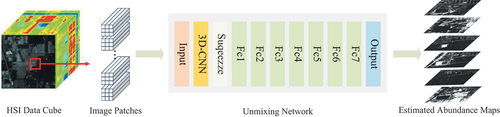
Hyperspectral images encompass both spectral and spatial information. By integrating spatial features, the unmixing algorithm can leverage contextual information from neighbouring pixels. Hence, 3D CNN is an ideal approach as it captures spatial-spectral patterns resulting from the spatial arrangement and spectral variations of materials. In our work, the proposed network structure combines 3D-CNN and MLP, as depicted in Figure 1. The 3D-CNN extracts the spatial-spectral features from image patches, and the MLP is a mapper from spatial-spectral features to fractional abundance. The input to the network is an image patch from the HSI, with the output representing the fractional abundance of the central pixel within the patch. The image patch has a size of $3\times 3\times \mathit{L}$, while the size of the convolving kernel is $3\times 3\times 3$. Since the kernel size matches the image patch, there is no need for a pooling layer to reduce the spatial dimension.

Figure 1. Structure of CNN-SsN unmixing network.

To ensure consistency between the processing of boundary pixels and internal pixels of the HSI, replication padding is employed to fill the boundaries of the HSI. Replication padding duplicates the edge pixels to generate additional rows and columns around the original image. Assuming the spatial size of HSI is $\mathit{w}\times \mathit{h}$, firstly, the technique duplicates the first and last columns, resulting in a size change to $\mathit{w}\times (\mathit{h}+2)$. Then, it duplicates the first and last rows. As a result, the final image size becomes $(\mathit{w}+2)\times (\mathit{h}+2)$. Padding enables the extraction of image patches for all pixels in the original HSI, ensuring that the number of training samples matches the number of pixels. Let $x_{(\mathit{i})}$ represent the image patch centred on the pixel at row $\mathit{p}$, column $\mathit{q}$.

The first layer of CNN-SsN consists of a 3D convolutional layer with valid padding. The size of input ${\mathbf{X}}^{(\mathit{p},\mathit{q})}$ is $3\times 3\times \mathit{L}$, and the output ${\mathbf{F}}^{(\mathit{p},\mathit{q})}$ has a size of $1\times 1\times (\mathit{L}-2)$. The $\mathit{l}$-th element of ${\mathbf{F}}^{(\mathit{p},\mathit{q})}$ can be expressed as:

(3) ${\mathbf{F}}_l^{(p,q)}=\mathrm{Conv}3\mathrm{d}({\mathbf{X}}^{(\mathit{p},\mathit{q})})=\mathrm{ReLU}(\sum _{\mathit{i}=0}^2\sum _{\mathit{j}=0}^2\sum _{\mathit{k}=0}^2{\mathbf{W}}_{\mathit{i},\mathit{j},\mathit{k}}{\mathbf{X}}_{i,j,l+k-1}^{(p,q)}+\mathit{b})$(3)

where $\mathbf{W}$ and $\mathit{b}$ are the convolving kernel’s weight and bias, respectively.

Prior to being input to the MLP, ${\mathbf{F}}^{(\mathit{p},\mathit{q})}$ is transformed into a 1-d vector $f^{(\mathit{p},\mathit{q})}$. MLP consists of a series of fully connected layers, followed by the SoftMax layer. The spatial-spectral features extracted by the convolutional network are further transformed by MLP, which map them to a layer with $\mathit{m}$ units. Detailed specifications can be found in Table 1. $\mathrm{F}{\mathrm{C}}_i$ layers can be expressed as follows:

(4) $f_i^{(p,q)}=\mathrm{ReLU}({\mathbf{W}}_i{f}_{i-1}^{(p,q)}+{\mathit{b}}_i),\mathit{i}=1,2,\dots ,7$(4)

Table 1. Structure of the proposed network.

CNN-SsN	Layers	Number of Kernels	Input Size	Output Size
3D-CNN part	Conv3d layer	1	$3\times 3\times \mathit{L}$	$1\times 1\times (\mathit{L}-2)$
MLP part	FC1 layer	–	$(\mathit{L}-2)$	90
	FC2 layer	–	90	60
	FC3 layer	–	60	30
	FC4 layer	–	30	$\mathit{m}$
	FC5 layer	–	$\mathit{m}$	$\mathit{m}$
	FC6 layer	–	$\mathit{m}$	$\mathit{m}$
	SoftMax layer	–	$\mathit{m}$	$\mathit{m}$

Where ${\mathbf{W}}_i$, ${\mathit{b}}_i$ are the weight and bias of $\mathrm{F}{\mathrm{C}}_i$, $f_i^{(p,q)}$ is the output of $\mathrm{F}{\mathrm{C}}_i$. The SoftMax layer is presented below:

(5) $\hat{a}=\mathrm{Softmax}(\mathit{z})=\frac{{\mathit{e}}^{\mathit{z}}}{{\sum }_{k=1}^m{e}^{{\mathit{z}}_i}}$(5)

where $\mathit{z}\in R^{1\text{timesm}}$ is the output of the last FC layer. The SoftMax layer ensures that ANC and ASC are met. To sum up, the proposed network is formatted as followed:

(6) $\hat{a}={\phi }_{\theta }({\mathbf{X}}^{(\mathit{p},\mathit{q})})$(6)

Where $\stackrel{\mathit{ˆ}}{a}$ is the output of the network, and it can represent the fractional abundance. $\mathit{\theta }$ represents all trainable parameters in the network.

2.2.2. Loss function

After determining the network structure, the next step is parameter optimization, which aims to minimize the error between network output and the corresponding label by learning useful latent correlations from data. Considering the limited availability of labelled training samples, this study adopts a semi-supervised training approach for the network. Specifically, the training samples are divided into two parts: labelled samples and unlabelled samples. Labelled samples constitute only approximately 5% of the total training samples, while the remaining samples are considered as unlabelled. To utilize the unlabelled data for training purpose, we specifically design a dedicated loss function.

For labelled data, we use Mean Square Error (MSE) and Normalized Abundance Angle Distance (NAAD). MSE is defined as follows:

(7) $J_{\mathrm{M}\mathrm{S}\mathrm{E}}^{\mathrm{S}\mathrm{u}\mathrm{p}}=\frac{1}{n_1}\sum _{\mathit{i}=1}^{n_1}({\hat{a}}^{\mathit{i}}-{\mathit{a}}^i{)}^2$(7)

where $n_1$ denotes the number of labelled samples, ${\hat{a}}^{\mathit{i}}$ and $a^i$ represent the prediction and label of the $i^{\mathit{th}}$ labelled sample, respectively. Normalized Abundance Angle Distance (NAAD) is expressed as:

(8) $J_{\mathrm{N}\mathrm{A}\mathrm{A}\mathrm{D}}^{\mathrm{S}\mathrm{u}\mathrm{p}}=\frac{1}{n_1}\sum _{\mathit{i}=1}^{n_1}{D}_{\mathrm{KL}}({\hat{\mathbf{a}}}^{\mathit{i}},{\mathbf{a}}^i)$(8)

(9) $D_{\mathrm{KL}}({\hat{\mathbf{a}}}^{\mathit{i}},{\mathbf{a}}^i)=\mathit{L}({\hat{\mathbf{a}}}^{\mathit{i}},{\mathbf{a}}^i)log(\mathit{L}({\hat{\mathbf{a}}}^{\mathit{i}},{\mathbf{a}}^i))$(9)

(10) $\mathit{L}({\hat{\mathbf{a}}}^{\mathit{i}},{\mathbf{a}}^i)=1-\frac{\mathit{C}({\hat{\mathbf{a}}}^{\mathit{i}},{\mathbf{a}}^i)}{\mathit{\pi }}$(10)

(11) $\mathit{C}({\hat{\mathbf{a}}}^{\mathit{i}},{\mathbf{a}}^i)={cos}^{-1}\left(\frac{{\mathit{a}}^i\cdot {\mathit{a}}^i}{\parallel {\mathit{a}}^i{\parallel }_2\cdot \parallel {\mathit{a}}^i{\parallel }_2}\right)$(11)

For unlabelled data, the loss function includes terms: MSE and Normalized Spectral Angle Distance (NSAD). The central pixel of the input image patch is reconstructed by the known endmembers matrix $\mathbf{E}$:

(12) ${\hat{\mathbf{X}}}_{\mathrm{centre}}^{\mathit{i}}={\hat{\mathbf{a}}}^{\mathit{i}}\mathbf{E}$(12)

where ${\hat{\mathbf{X}}}_{\mathrm{centre}}^{\mathit{i}}$ is the reconstructed pixel and ${\mathbf{X}}_{\mathrm{c}\mathrm{e}\mathrm{ntre}}^i$ is the central pixel of the input patch ${\mathbf{X}}^i$. MSE and NSAD for unlabelled data are formulated as follows:

(13) $J_{\mathrm{M}\mathrm{S}\mathrm{E}}^{\mathrm{U}\mathrm{n}\mathrm{Sup}}=\frac{1}{n_2}\sum _{\mathit{i}=1}^{n_2}({\hat{\mathbf{X}}}_{\mathrm{centre}}^{\mathit{i}}-{\mathbf{X}}_{\mathrm{c}\mathrm{e}\mathrm{ntre}}^i{)}^2$(13)

(14) $J_{\mathrm{N}\mathrm{S}\mathrm{A}\mathrm{D}}^{\mathrm{U}\mathrm{n}\mathrm{Sup}}=\frac{1}{n_2}\sum _{\mathit{i}=1}^{n_2}{D}_{\mathrm{KL}}({\hat{\mathbf{X}}}_{\mathrm{centre}}^{\mathit{i}},{\mathbf{X}}_{\mathrm{c}\mathrm{e}\mathrm{ntre}}^i)$(14)

where $n_2$ denotes the number of unlabelled samples.

The above formulas measure the similarity between the reconstructed pixel and the central pixel of the input patch. To make full use of the neighbourhood information, we design the Neighbourhood Similarity (NS). Within an image patch, there exists a certain degree of similarity between the central pixel and its neighbouring pixels. To quantify this similarity, we employ the Spectral Angle Distance (SAD) as a measurement between the central pixel and its neighbouring pixels. The similarity ${\delta }_k$ can be mathematically expressed as follows:

(15) ${\delta }_k=\frac{\frac{1}{C({\mathbf{X}}_k^i,{\mathbf{X}}_{\mathrm{c}\mathrm{entre}}^i)}}{{\sum }_{k\in U({\mathbf{X}}_{\mathrm{c}\mathrm{entre}}^i)}\frac{1}{C({\mathbf{X}}_k^i,{\mathbf{X}}_{\mathrm{c}\mathrm{entre}}^i)}}$(15)

where $\mathit{U}({\mathbf{X}}_{\mathrm{c}\mathrm{e}\mathrm{ntre}}^i)$ is the index set of the neighbourhood pixels, and ${\delta }_k$ represents the self-adaptive weight coefficient. Then, the NS term can be written as:

(16) $J_{\mathrm{NS}}=\frac{1}{N}\sum _{\mathit{i}=1}^N\left(\sum _{k\in U({\mathbf{X}}_{\mathrm{c}\mathrm{entre}}^i)}{\delta }_k{({\mathbf{X}}_k^i-{\hat{\mathbf{X}}}_{\mathrm{centre}}^{\mathit{i}})}^2\right)$(16)

where $\mathit{N}$ represents the total number of training samples, encompassing both labelled and unlabelled samples. This implies that the closer the neighbouring pixel resembles the central pixel, the stronger its impact on the reconstruction of the central pixel. In summary, the loss function for both labelled and unlabelled data is presented as follows:

(17) $J^{\mathrm{Sup}}={\lambda }_1\cdot J_{\mathrm{M}\mathrm{S}\mathrm{E}}^{\mathrm{S}\mathrm{u}\mathrm{p}}-{\lambda }_2\cdot J_{\mathrm{N}\mathrm{A}\mathrm{A}\mathrm{D}}^{\mathrm{S}\mathrm{u}\mathrm{p}}+{\lambda }_5\cdot J_{\mathrm{NS}}$(17)

(18) $J^{\mathrm{UnSup}}={\lambda }_3\cdot J_{\mathrm{M}\mathrm{S}\mathrm{E}}^{\mathrm{U}\mathrm{n}\mathrm{Sup}}-{\lambda }_4\cdot J_{\mathrm{N}\mathrm{S}\mathrm{A}\mathrm{D}}^{\mathrm{U}\mathrm{n}\mathrm{Sup}}+{\lambda }_5\cdot J_{\mathrm{NS}}$(18)

where ${\lambda }_1$ to ${\lambda }_5$ are hyperparameters that determine the extent to which each term influences parameter updates. The overall training framework of CNN-SsN is shown in Figure 2.

Figure 2. The overall training framework of CNN-SsN.

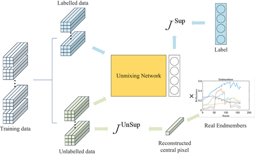
During the training process, the weights and biases of the convolutional and MLP layers are randomly initialized. The network weights are alternately updated using the $J^{\mathrm{Sup}}$ loss and $J^{\mathrm{UnSup}}$ loss. This alternating update process is repeated to obtain the final result.

2.2.3. GAN for generating labelled samples

To utilize the semi-supervised learning method, it is necessary to create two types of data: labelled and unlabelled data. However, in some scenarios, labelled data may be unavailable. To address this situation, we propose a scheme to generate synthetic labelled data that aligns with the actual data distribution. Subsequently, the generated data is used as labelled data, while the original real data serves as unlabelled data for conducting semi-supervised training and optimizing the unmixing network.

Commonly used generative networks for data generation include Generative Adversarial Networks (GANs) and Variational Autoencoder (VAE) (Kingma and Welling 2013). In our study, we utilize Wasserstein GAN (WGAN) (Arjovsky, Chintala, and Bottou 2017) as generative network. WGAN is a GAN variant that aims to enhance training stability and sample quality. The process of generating synthetic labelled samples is illustrated in Figure 3. The pale orange arrow represents the training process, and the blue arrow represents the generation process, which follows the training process. Before training, the traditional method R-CoNMF (Jun et al. 2016) is first used to obtain the pseudo-abundance map of the dataset, and then the pseudo-abundance patches sampled from this abundance map are fed into the generation network for training. Although these pseudo-abundance patches may not be completely accurate, they can represent the true abundance distribution to some extent. After training, the generator of GAN can generate abundance patches that resemble the real abundance distribution. These generated abundance patches are then multiplied with real endmembers to construct synthetic image patches, which are treated as labelled samples. With the generated labelled samples, we can training the network as shown in Figure 2.

Figure 3. Diagram of the process of generating synthetic label data.

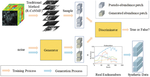
WGAN employs Wasserstein distance as its objective function, which addresses issues of training instability and mode collapse commonly encountered in traditional GANs. Wasserstein distance provides a smoother and more mathematically tractable measure of discrepancy between the generated sample distribution and the real sample distribution. To achieve this, WGAN introduces a constraint on the discriminator parameters, necessitating it to be a Lipschitz continuous function. This constraint is enforced through weight clipping or gradient penalty, thereby ensuring that the gradients of the discriminator remain bounded. By imposing this constraint, WGAN achieves a more stable training process and facilitates improved coordination between the generator and discriminator training.

3. Result

This section applies the proposed method to one synthetic dataset and two real datasets. One of the real datasets do not have any labelled data. We begin by introducing the datasets employed, followed by an introduction to the comparison methods and evaluation metrics. Finally, we present the experimental results.

3.1. Hyperspectral dataset

3.1.1. Synthetic dataset

We propose a dataset synthesis method that utilizes superpixel segmentation and random splitting. Superpixels, produced by superpixel segmentation, are pivotal for generating synthetic datasets with specific structural characteristics. Pixels in superpixels have two main structural characteristics. First, they provide the smoothness of spatial position. Second, they maintain the structural similarity of abundance vectors, which are often composed of the same group of endmembers. These characteristics enable us to generate synthetic images with locally smooth spatial structures, a crucial factor for achieving realistic synthetic data. Random splitting doubles the number of generated abundance maps, introducing randomness for more diverse synthetic datasets. Furthermore, splitting applied to superpixels can retain the structural characteristics, including spatial smoothness and the structural similarity of abundance, found within pixels in the same superpixel. This method enables the creation of a synthetic dataset with inherent spatial structure information, facilitating effective verification of the proposed method’s superiority. The specific steps of the synthesis process are outlined below:

1. Unmixing the basic real dataset: An existing hyperspectral dataset serves as the basic dataset, and the unmixing results of the basic dataset are obtained using FCLS. This yields $\mathit{m}$ abundance maps, where $\mathit{m}$ represents the number of endmembers in the basic dataset.

2. Superpixel segmentation for each abundance map: The abundance maps obtained from step 1 are treated as greyscale images. Superpixel segmentation is then applied to each greyscale image using the Simple Linear Iterative Clustering (SLIC) algorithm(Achanta et al. 2012).

3. Random splitting of the superpixel segmentation results: For each superpixel block, a self-defined threshold $\mathit{\theta }$, and two random numbers $\mathit{a}$ and $\mathit{b}$ between 0 and 1 are generated. The superpixel block will be split into two blocks based on the following conditions: when $\mathit{a}$ is greater than $\mathit{\theta }$, the values of the two resulting blocks after splitting are $y_1=\mathit{y}(1-\mathit{b})$ and $y_2=\mathit{yb}$, respectively; when $\mathit{a}$ is less than or equal to $\mathit{q}$, the values of the blocks are $y_1=\mathit{y}$ and $y_2=0$, respectively.

4. Selection of endmembers from a spectral library to synthesize the data: After splitting all the superpixel blocks, the number of abundance maps is doubled. $2\mathit{m}$ endmembers are randomly selected from the spectral library and multiplied by the abundance maps to generate the synthetic dataset.

5. Addition of additive white Gaussian noise: Gaussian noise with a signal-to-noise ratio (SNR) of 20 dB is added to all bands.

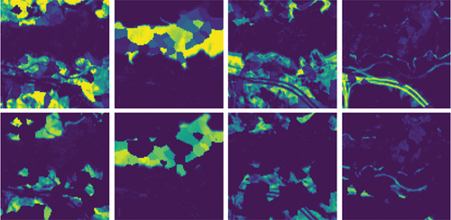
The synthesis method employs superpixel segmentation to ensure that the resulting abundance map exhibits a spatial neighbourhood structure in the base dataset. In this study, we utilize the Jasper Ridge (Zhu et al. 2014) dataset as the foundational dataset, which comprises $100\times 100$ pixels and 224 spectral bands. It contains four distinct endmembers: Road, soil, tree, and water. Following the splitting process, the number of endmembers increases to eight. Figures 4 and 5 depict the abundance maps obtained through FCLS for Jasper Ridge and the synthetic dataset, respectively. In summary, the synthesized hyperspectral image has dimensions of $100\times 100$ pixels. It consists of eight randomly selected endmembers from the spectral library, with each endmember comprising 198 spectral channels.

Figure 4. The estimated abundance maps on Jasper Ridge.

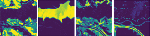
Figure 5. The abundance maps after superpixel segmentation and random splitting.

3.1.2. Urban

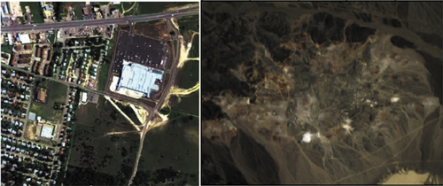
The Urban dataset (Zhu 2017) is widely used in hyperspectral unmixing research. The pseudo-colour image of the urban area is presented in the left section of Figure 6. It was acquired in October 1995, covering an urban area located in Corpus Christi Bay, Texas, U.S.A.. The image has dimensions of $307\times 307$ pixels, with each pixel representing a real area of 2 square metres. Certain bands, specifically bands 1–4, 76, 87, 101–111, 136–153, and 198–210, suffer from poor quality due to water vapour absorption and atmospheric effects. These bands are typically excluded in practical applications, resulting in a remaining set of 162 bands. The Urban dataset consists of three versions: the 4-Endmember version, 5-Endmember version, and 6-Endmember version. In our study, we utilize the 6-Endmember version, which includes soil, tree, asphalt road, roof, metal, and grass.

Figure 6. The pseudo-color images of real dataset. Urban(left), Cuprite(right).

3.1.3. Cuprite

The Cuprite dataset (Qian et al. 2011) is widely regarded as one of the most representative datasets. The pseudo-colour image of the cuprite is presented in the right section of Figure 6. It was collected in Nevada in 1997, providing real-world data for analysis. In our study, we utilize a subgraph with dimensions of $250\times 191$ pixels. The dataset comprises 224 bands covering the wavelength range of 0.4 µm to 2.5 µm. However, certain bands, specifically bands 1–2, 104–113, 148–167, and 221–224, suffer from poor quality due to noise and environmental factors. Consequently, these bands are excluded, resulting in the retention of 188 bands. Notably, the Cuprite dataset consists of 12 distinct endmembers, and no labelled data is available.

3.2. Comparison methods and evaluation metrics

To evaluate the effectiveness of the proposed method, we compare it with six widely adopted methods: Minimum Volume Constrained Nonnegative Matrix Factorization (MVCNMF), SUnSAL, Collaborative Sparse Unmixing via Variable Splitting and Augmented Lagrangian (CLSUnSAL) (Iordache, Bioucas-Dias, and Plaza 2014), Subspace Unmixing With Low-Rank Attribute (SULoRA) (Hong and Xiang Zhu 2018), Autoencoder for Unmixing(AE) (Burkni et al. 2018), and Hyperspectral unmixing using Deep Image Prior(UnDIP) (Rasti et al. 2021).

The unmixing results are assessed using three evaluation metrics: mean square error (MSE), abundance angle distance (AAD), and spectral angle distance (SAD). MSE quantifies the errors between the predicted vector and the true label vector, while AAD and SAD measure the structural similarity between the predicted vector and the target vector. The formulas for these metrics are as follows:

(19) $\mathrm{MSE}=\frac{{\sum }_{i=1}^N{({\hat{\mathbf{a}}}^{\mathit{i}}-{\mathbf{a}}^i)}^2}{\mathit{N}}$(19)

(20) $\mathrm{AAD}={cos}^{-1}(\frac{{\hat{\mathbf{a}}}^{\mathit{i}}\cdot {\mathbf{a}}^i}{\parallel {\mathit{a}}^i{\parallel }_2\cdot \parallel {\mathit{a}}^i{\parallel }_2})$(20)

(21) $\mathrm{SAD}={cos}^{-1}(\frac{{\hat{\mathbf{x}}}^{\mathit{i}}\cdot {\mathbf{x}}^i}{\parallel {\mathbf{x}}^i{\parallel }_2\cdot \parallel {\mathbf{x}}^i{\parallel }_2})$(21)

3.3. Experimental result

3.3.1. Synthetic dataset

The synthetic dataset consists of 10,000 training samples. Among these, 500 image patches are randomly assigned as labelled data, representing 5% of the total training samples, while the remaining 95% are treated as unlabelled data. The hyperparameters ${\lambda }_1$ to ${\lambda }_5$ in the loss function are set to 0.8, 0.2, 0.1, 0.1, and 0.001, respectively. Both the labelled data’s loss and the unlabelled data’s loss use a learning rate of 0.001.

The MSE results of hyperspectral unmixing using different algorithms are presented in Table 2. Our proposed method, CNN-SsN, achieves the lowest mean value of 0.0011. And CNN-SsN demonstrates superior performance in most abundance maps, except for abundance maps #6 and #8. Table 3 displays the AAD results, revealing that UnDIP and SUnSAL perform well in abundance maps #6 and #8, respectively, while CNN-SsN outperforms other methods in the remaining six maps, with an mean AAD value of 0.1456. Compared to the suboptimal result, CNN-SsN shows a performance improvement of 10.1%. Furthermore, qualitative comparisons in Figure 7 clearly illustrate the higher accuracy of the proposed method in detail for abundance maps corresponding to endmembers 1, 2, 4, and 7. In summary, our proposed CNN-SsN outperforms other comparison methods in terms of performance.

Figure 7. Visualization of the abundance maps obtained by different methods on synthetic dataset.

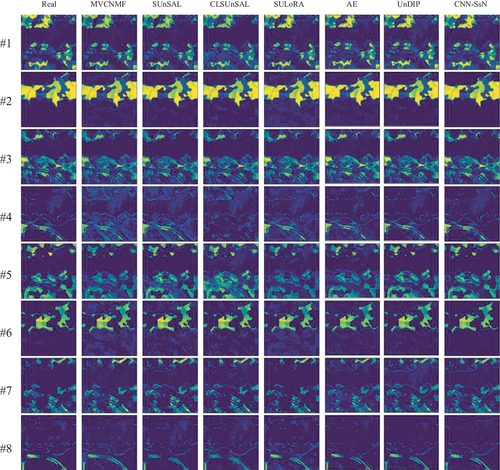
Table 2. Mean square error (MSE) results on synthetic dataset, the best result in bold.

Method	MVCNMF	SUnSAL	CLSUnSAL	SULoRA	AE	UnDIP	CNN-SsN
#1	0.0057±00.04%	0.0042±00.15%	0.0101±00.00%	0.0034±00.20%	0.0021±00.01%	0.0010±00.00%	0.0008±00.01%
#2	0.0014±00.01%	0.0011±00.04%	0.0014±00.00%	0.0010±00.03%	0.0012±00.03%	0.0007±00.00%	0.0006±00.01%
#3	0.0050±00.08%	0.0024±00.13%	0.0035±00.00%	0.0021±00.06%	0.0013±00.01%	0.0012±00.00%	0.0007±00.01%
#4	0.0108±00.27%	0.0092±00.50%	0.0270±00.00%	0.0099±01.03%	0.0027±00.03%	0.0012±00.00%	0.0011±00.01%
#5	0.0157±00.36%	0.0171±00.66%	0.0206±00.00%	0.0132±00.99%	0.0040±00.05%	0.0031±00.00%	0.0018±00.02%
#6	0.0020±00.02%	0.0045±00.27%	0.0013±00.00%	0.0029±00.14%	0.0015±00.01%	0.0005±00.00%	0.0007±00.00%
#7	0.0021±00.03%	0.0038±00.23%	0.0029±00.00%	0.0028±00.19%	0.0038±00.01%	0.0032±00.00%	0.0014±00.02%
#8	0.0023±00.02%	0.0013±00.02%	0.0033±00.00%	0.0023±00.26%	0.0033±00.02%	0.0016±00.00%	0.0022±00.01%
Mean	0.0056±00.09%	0.0055±00.16%	0.0088±00.00%	0.0047±00.27%	0.0025±00.01%	0.0016±00.00%	0.0011±00.01%

Table 3. Abundance Angle Distance (AAD) results on synthetic dataset, the best result in bold.

Method	MVCNMF	SUnSAL	CLSUnSAL	SULoRA	AE	UnDIP	CNN-SsN
#1	0.1013±00.56%	0.1540±03.16%	0.2599±00.00%	0.1399±05.81%	0.1289±00.21%	0.0914±00.03%	0.0797±00.54%
#2	0.0713±00.50%	0.0764±01.30%	0.0829±00.00%	0.0723±01.39%	0.0807±00.92%	0.0585±00.02%	0.0563±00.35%
#3	0.1109±00.55%	0.1244±04.66%	0.1699±00.00%	0.1270±02.21%	0.1303±00.57%	0.1174±00.02%	0.0951±00.54%
#4	0.6653±06.17%	0.5451±10.16%	1.3097±00.00%	0.5622±29.60%	0.3304±02.13%	0.2262±00.06%	0.2141±00.67%
#5	0.3424±03.31%	0.3880±08.27%	0.4526±00.00%	0.2804±15.84%	0.1817±01.01%	0.1828±00.01%	0.1145±00.75%
#6	0.1695±00.71%	0.2389±07.37%	0.1377±00.00%	0.1921±05.02%	0.1426±00.31%	0.0880±00.02%	0.0980±00.23%
#7	0.2189±01.21%	0.2534±05.02%	0.2633±00.00%	0.2448±06.90%	0.3007±00.41%	0.2736±00.05%	0.1772±00.96%
#8	0.3071±01.19%	0.2390±02.89%	0.4047±00.00%	0.2639±13.36%	0.4104±01.14%	0.2576±00.11%	0.3302±00.99%
Mean	0.2483±01.23%	0.2524±02.66%	0.3851±00.00%	0.2353±07.05%	0.2132±00.43%	0.1619±00.02%	0.1456±00.45%

3.3.2. Urban

The urban dataset contains 94,249 pixels. In this experiment, 5,000 image patches are randomly selected as labelled training samples, accounting for 5.3% of the total data. The remaining samples are considered unlabelled data, and no real labels were provided during training. For this dataset, the loss function parameters ${\lambda }_1$ to ${\lambda }_5$ are set to 0.09, 0.09, 0.01, 0.01, and 0.0001, respectively. The learning rates for labelled and unlabelled training loss are set to 0.0009 and 0.001, respectively.

Table 4 presents the MSE results for all selected methods on the urban dataset. Of particular note is the performance of the proposed CNN-SsN method. It exhibits a substantial and noteworthy improvement, achieving a remarkable 48.5% enhancement in accuracy compared to the suboptimal performance as indicated by the mean MSE. Delving into the specifics of the abundance map results, it becomes vividly evident that CNN-SsN consistently outpaces its contemporaries across the majority of abundance maps. While it’s crucial to acknowledge the proficiency of other methods, such as MVCNMF’s excellence in”dirt” abundance map estimation, AE’s adeptness in”roof” abundance maps, and SULoRA’s proficiency in”metal” abundance map estimation, our method exhibits competitive performance in these specific abundance maps.

Table 4. Mean square error (MSE) results on Urban, the best result in bold.

Method	MVCNMF	SUnSAL	CLSUnSAL	SULoRA	AE	UnDIP	CNN-SsN
Dirt	0.0048±00.05%	0.0627±00.01%	0.0227±00.00%	0.0461±00.23%	0.0182±00.07%	0.0226±00.00%	0.0067±00.06%
Tree	0.0387±00.45%	0.0198±00.29%	0.0308±00.00%	0.0098±00.03%	0.0046±00.07%	0.0319±00.01%	0.0044±00.09%
Asphalt Road	0.0259±00.08%	0.0927±00.26%	0.1099±00.00%	0.0746±00.36%	0.0251±00.15%	0.1129±00.05%	0.0079±00.10%
Roof	0.0166±00.15%	0.0033±00.01%	0.0208±00.00%	0.0050±00.01%	0.0013±00.01%	0.0214±00.00%	0.0017±00.02%
Metal	0.0045±00.06%	0.0107±00.09%	0.0092±00.00%	0.0023±00.00%	0.0032±00.06%	0.0125±00.10%	0.0038±00.01%
Grass	0.0134±00.16%	0.0301±00.52%	0.0355±00.00%	0.0184±00.08%	0.0083±00.10%	0.0371±00.03%	0.0066±00.14%
Mean	0.0173±00.11%	0.0365±00.19%	0.0382±00.00%	0.0260±00.12%	0.0101±00.03%	0.0397±00.03%	0.0052±00.04%

The AAD results are shown in Table 5. The proposed CNN-SsN achieves an mean AAD value of 0.2672, corresponding to a 15.6% improvement over suboptimal methods. For the specific abundance map results, MVCNMF demonstrates strong performance in soil abundance, AE yields favourable results for roof map, and SULoRA excels in metal map. In the remaining three maps, the proposed CNN-SsN achieves superior results. Figure 8 depicts the visualization of the abundance maps. Overall, CNN-SsN produces abundance maps that closely resemble the real abundance maps. In the asphalt road’s abundance map, CNN-SsN accurately distinguishes between roads and houses, yielding superior visual effects for roads. Moreover, CNN-SsN provides better analysis of grass in the lower left corner of the abundance map compared to other methods.

Figure 8. Visualization of the abundance maps obtained by different methods on Urban.

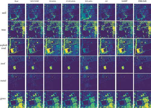
Table 5. Abundance Angle Distance (AAD) results on Urban, the best result in bold.

Method	MVCNMF	SUnSAL	CLSUnSAL	SULoRA	AE	UnDIP	CNN-SsN
Dirt	0.2438±00.65%	1.5232±00.35%	0.6450±00.00%	0.6230±00.94%	0.5700±01.16%	0.6432±00.03%	0.3121±01.61%
Tree	0.4520±00.65%	0.2670±01.79%	0.4336±00.00%	0.2329±00.26%	0.1582±00.81%	0.4408±00.08%	0.1547±01.63%
Asphalt Road	0.4548±01.00%	0.6337±00.26%	0.7274±00.00%	0.6132±02.82%	0.4165±00.89%	0.7297±00.05%	0.2404±01.49%
Roof	0.6303±01.12%	0.2067±00.05%	0.7341±00.00%	0.3191±00.38%	0.1607±00.80%	0.7458±00.10%	0.1925±00.87%
Metal	0.5884±00.80%	0.9486±07.95%	0.9202±00.00%	0.4098±00.24%	0.4697±03.30%	1.1087±04.14%	0.5438±00.25%
Grass	0.2025±00.82%	0.3042±02.41%	0.3469±00.00%	0.1934±00.17%	0.1789±01.00%	0.3578±00.14%	0.1596±01.57%
Mean	0.4287±00.56%	0.6472±02.12%	0.6346±00.00%	0.3986±00.80%	0.3257±00.79%	0.6710±00.72%	0.2672±00.43%

Based on these results, it can be concluded that CNN-SsN delivers highly competitive outcomes when compared to other methods on urban dataset.

3.3.3. Cuprite

The Cuprite dataset consists of 47,750 pixels and does not have abundance labels for training samples. To generate synthetic labelled data, we employ Wasserstein Generative Adversarial Networks (WGAN). Initially, the traditional unmixing method, R-CoNMF, is used to obtain a pseudo-abundance map. The abundance patches extracted from the pseudo-abundance map are then used as training data for the WGAN. Through training, the generator of WGAN is able to generate abundance patches that align with the true abundance distribution. These generated patches are multiplied with the actual endmembers to construct synthetic image patches.

The synthetic image patches serve as labelled data, while the real image patches are used as unlabelled data for CNN-SsN training. The generator has the ability to generate an unlimited number of synthetic image patches with abundance labels. To balance the impact of real and synthetic data during training, the number of synthetically labelled samples is set to match the amount of raw unlabelled data, which totals 47,750 samples. In the Cuprite dataset, the loss hyperparameters ${\lambda }_1$ to ${\lambda }_5$ are set to 0.8, 0.2, 0.1, 0.1, and 0.001, respectively. The learning rates for labelled and unlabelled data are 0.0001 and 0.001, respectively.

Since true abundance labels are unavailable, the unmixing result is multiplied by the reference endmember to obtain the reconstructed pixel. The Mean Square Error (MSE) and Spectral Angle Distance (SAD) are used to evaluate the unmixing performance by measuring the errors between the reconstructed and original pixels. The results are recorded in Table 6. Compared with other methods, the proposed CNN-SsN achieves the best MSE result of 0.0002, representing 50% improvement over the suboptimal result. Regarding SAD, the proposed CNN-SsN also outperforms other methods, while UnDIP yields suboptimal result.Figure 9 illustrates the resulting abundance maps by CNN-SsN.

Figure 9. Visualization of the abundance maps obtained by the proposed method on Cuprite.

Table 6. Mean square error (MSE) and spectral Angle Distance (SAD) results on Cuprite dataset, the best result in bold.

Method	MVCNMF	SUnSAL	CLSUnSAL	SULoRA	AE	UnDIP	CNN-SsN
MSE	0.0015±00.02%	0.0017±00.02%	0.0097±00.00%	0.0138±00.07%	0.0031±00.07%	0.0004±00.00%	0.0002±00.01%
SAD	0.0645±00.30%	0.0988±01.15%	0.0863±00.00%	0.1339±00.44%	0.0862±01.74%	0.0466±00.23%	0.0258±00.45%

3.3.4. Ablation experiment

This section presents the results of an ablation experiment in Table 7, aimed at dissecting the contributions of the components in our semi-supervised loss function. The experiment evaluates the functions of the ’Supervised Part’, ’Unsupervised Part’, and ’NS Term’ within our semi-supervised loss. We assessed performance using MSE and AAD on the Syndata and Urban datasets.

Table 7. Ablation experiment results.

Experiment Group	supvised part	unsupvised part	NS term	MSE on syndata	AAD on syndata	MSE on Urban	AAD on Urban
Ablation Group 1	✓			0.0029	0.2305	0.0071	0.3299
Ablation Group 2	✓	✓		0.0013	0.1513	0.0055	0.2724
Baseline Group	✓	✓	✓	0.0011	0.1465	0.0052	0.2672

We established three experimental groups. The Baseline Group, comprising all components, demonstrated the best performance with the lowest MSE and AAD on both datasets, indicating superior performance. Conversely, Ablation Group 1, which excluded the ’Unsupervised Part’ and ’NS Term’, exhibited increased errors, underscoring their significance. Additionally, Ablation Group 2, which retained only the ’Supervised Part’ and ’Unsupervised Part’ while omitting the ’NS Term’, showed a slight increase in errors compared to the Baseline Group. These findings indicate a positive contribution from the ’Unsupervised Part’ and ’NS Term’ to our method’s performance on these datasets.

4. Discussion

The proposed CNN-SsN demonstrates strong performance on both synthetic and real datasets, highlighting its superiority over traditional blind source unmixing methods. Unlike conventional approaches that focus solely on decomposing individual pixels without considering contextual information, our method leverages the 3D-CNN architecture to capture both spatial and spectral neighbourhood information of the target pixel. This integration of spatial and spectral features provides a significant advantage over single-pixel-based unmixing methods.

While unsupervised deep learning models, particularly Autoencoders, are prevalent in the current literature for hyperspectral unmixing (HU), they often suffer from being trapped in local optima due to random weight initialization. In contrast, supervised methods tend to yield superior results, but the availability of labelled data is often limited. To address this challenge, we propose a semi-supervised learning approach that effectively utilizes a small percentage (5%) of labelled data while maximizing the utility of unlabelled data for auxiliary training. Furthermore, in scenarios where labelled data is unavailable, we employ Generative Adversarial Networks (GANs) to indirectly generate synthetic data with pseudo-labels, enabling their utilization as labelled data in our semi-supervised learning framework. Experimental results demonstrate the competitiveness of our method.

Overall, our proposed method combines the strengths of 3D-CNN for capturing spatial-spectral information and the benefits of semi-supervised learning for effectively leveraging limited labelled data. This approach yields highly competitive results in hyperspectral unmixing tasks.

Although the CNN-SsN algorithm presented in this study offers substantial advantages in abundance estimation, it is essential to recognize a notable limitation: our method relies on known real endmembers. The incorporation of real endmembers was a deliberate choice, aimed at improving the accuracy of abundance estimation by closely representing the actual materials within hyperspectral scenes. However, it is equally important to acknowledge that this reliance introduces specific constraints. For instance, a dependence on fixed endmembers may restrict the algorithm’s adaptability to changing environmental conditions. Addressing this limitation presents an exciting avenue for future research, where techniques for more dynamic and accurate endmembers acquisition could be explored. These advances would enable the algorithm to better adapt to evolving scene compositions and environmental factors. In summary, the reliance on real endmembers stands as a noteworthy constraint within our algorithm. Nevertheless, this limitation serves as an open invitation for further research to enhance the algorithm’s adaptability and overall performance. We firmly believe that tackling this challenge will significantly contribute to the ongoing progress in hyperspectral unmixing techniques.

5. Conclusion

This study addresses the challenge of hyperspectral unmixing with limited labelled samples by proposing an unmixing method that combines 3D-CNN and a semi-supervised learning method. The 3D-CNN is utilized to extract both spatial and spectral neighbourhood features of the central pixel. To overcome the limitations imposed by the scarcity of labelled samples, the network is trained in a semi-supervised manner, only leveraging a small amount of labelled data. In cases where the dataset lacks any labelled samples, a GAN is employed to generate synthetic training samples with labels that exhibit similar spatial structures to real data. Experimental results obtained from synthetic and real datasets demonstrate the superior unmixing performance of the proposed method.

Disclosure statement

No potential conflict of interest was reported by the author(s).

Additional information

Funding

This work was supported in part by the National Natural Science Foundation of China under Grant 61877066, in part by the Aero-Science Fund under Grant 20175181013 and in part by the Science and technology plan project of Xi’an under Grant 21RGZN0010.

References

- Achanta, R., A. Shaji, K. Smith, A. Lucchi, P. Fua, and S. Süsstrunk. 2012. “SLIC Superpixels Compared to State-Of-The-Art Superpixel Methods.” IEEE Transactions on Pattern Analysis and Machine Intelligence 34 (11): 2274–2282. November. Accessed September 19, 2019. https://doi.org/10.1109/tpami.2012.120.
- Arjovsky, M., S. Chintala, and L. Bottou. 2017. “Wasserstein Generative Adversarial Networks.” proceedings.mlr.press. July. https://proceedings.mlr.press/v70/arjovsky17a.html.
- Bioucas-Dias, J. M., and T. Figueiredo. 2010. “Alternating Direction Algorithms for Constrained Sparse Regression: Application to Hyperspectral Unmixing.” Workshop on Hyperspectral Image and Signal Processing: Evolution in Remote Sensing. June. Accessed April 25, 2023. https://doi.org/10.1109/whispers.2010.5594963.
- Bioucas-Dias, J. M., A. Plaza, N. Dobigeon, M. Parente, D. Qian, P. D. Gader, and J. Chanussot. 2012. “Hyperspectral Unmixing Overview: Geometrical, Statistical, and Sparse Regression-Based Approaches.” IEEE Journal of Selected Topics in Applied Earth Observations & Remote Sensing 5 (2): 354–379. May. https://doi.org/10.1109/jstars.2012.2194696.
- Burkni, P., J. Sigurdsson, J. R. Sveinsson, and M. O. Ulfarsson. 2018. “Hyperspectral Unmixing Using a Neural Network Autoencoder.” Institute of Electrical and Electronics Engineers Access 6:25646–25656. https://doi.org/10.1109/access2018.2818280. Accessed July 21, 2021.
- Chalen, T. M., and B. X. Vintimilla. 2019. “Towards Action Prediction Applying Deep Learning.” Paper presented at the 2019 IEEE Latin American Conference on Computational Intelligence (LA-CCI). November. Accessed July 11, 2023. https://doi.org/10.1109/la-cci47412.2019.9037051.
- Chen, L., G. Baozhen, and Y. Guo. 2017. “Nonlinear Unmixing of Hyperspectral Images Based on Differential Search Algorithm.” ACTA ELECTONICA SINICA 45:337–345. https://doi.org/10.3969/j.issn.0372-2112.2017.02.011.
- Cracknell, A. P. 1998. “Review Article Synergy in Remote Sensing-What’s in a Pixel?” International Journal of Remote Sensing 19 (11): 2025–2047. January. https://doi.org/10.1080/014311698214848
- Ding, C., and D. Tao. 2018. “Trunk-Branch Ensemble Convolutional Neural Networks for Video-Based Face Recognition.” IEEE Transactions on Pattern Analysis and Machine Intelligence 40 (4): 1002–1014. April. Accessed November 5, 2021. https://doi.org/10.1109/TPAMI.2017.2700390.
- Goodfellow, I., J. Pouget-Abadie, M. Mirza, X. Bing, D. Warde-Farley, S. Ozair, A. Courville, and Y. Bengio. 2020. “Generative Adversarial Networks.” Communications of the ACM 63 (11): 139–144. October. https://doi.org/10.1145/3422622.
- Heinz, D. C., and C. I. Chang. 2001. “Fully Constrained Least Squares Linear Spectral Mixture Analysis Method for Material Quantification in Hyperspectral Imagery.” IEEE Transactions on Geoscience & Remote Sensing 39 (3): 529–545. March. Accessed December 14, 2019. https://doi.org/10.1109/36.911111.
- Hong, D. F., and X. Xiang Zhu. 2018. “SULoRa: Subspace Unmixing with Low-Rank Attribute Embedding for Hyperspectral Data Analysis.” IEEE Journal of Selected Topics in Signal Processing 12 (6): 1351–1363. December. Accessed July 11, 2023. https://doi.org/10.1109/jstsp.2018.2877497.
- Iordache, M.-D., J. M. Bioucas-Dias, and A. Plaza. 2014. “Collaborative Sparse Regression for Hyperspectral Unmixing.” IEEE Transactions on Geoscience and Remote Sensing 52 (1): 341–354. January. Accessed January 12, 2023. https://doi.org/10.1109/tgrs.2013.2240001.
- Jin, Q., M. Yong, F. Fan, J. Huang, X. Mei, and M. Jiayi 2021. “Adversarial Autoencoder Network for Hyperspectral Unmixing.” IEEE Trans Neural Netw Learn Syst PP 1–15. January. Accessed July 11, 2023. https://doi.org/10.1109/tnnls.2021.3114203.
- Jun, L., J. M. Bioucas-Dias, A. Plaza, and L. Liu. 2016. “Robust Collaborative Nonnegative Matrix Factorization for Hyperspectral Unmixing.” IEEE Transactions on Geoscience and Remote Sensing 54 (10): 6076–6090. October. Accessed January 12, 2023. https://doi.org/10.1109/tgrs.2016.2580702.
- Kaliyar, R. K. 2020. “A Multi-Layer Bidirectional Transformer Encoder for Pre-Trained Word Embedding: A Survey of BERT.” IEEE Xplore. January. Accessed Novem- ber 30, 2020. https://ieeexplore.ieee.org/document/9058044/.
- Keshava, N., and J. F. Mustard. 2002. “Spectral Unmixing.” IEEE Signal Processing Magazine 19 (1): 44–57. January. https://doi.org/10.1109/79.974727.
- Kingma, D. P., and M. Welling. 2013. “Auto-Encoding Variational Bayes.” arXiv (Cornell University) 34. December. https://doi.org/10.48550/arxiv.1312.6114.
- Landgrebe, D. 2002. “Hyperspectral Image Data Analysis.” IEEE Signal Processing Magazine 19 (1): 17–28. https://doi.org/10.1109/79.974718. Accessed May 4, 2021.
- Ozkan, S., B. Kaya, and G. Bozdagi Akar. 2019. “EndNet: Sparse AutoEncoder Network for Endmember Extraction and Hyperspectral Unmixing.” IEEE Transactions on Geoscience and Remote Sensing 57 (1): 482–496. January. Accessed July 9, 2023. https://doi.org/10.1109/tgrs.2018.2856929.
- Palsson, B., M. O. Ulfarsson, and J. R. Sveinsson. 2021. “Convolutional Autoencoder for Spectral–Spatial Hyperspectral Unmixing.” IEEE Transactions on Geoscience and Remote Sensing 59 (1): 535–549. January. Accessed July 11, 2023. https://doi.org/10.1109/tgrs.2020.2992743.
- Pauca, V., J. P. Paul, and J. P. Robert. 2006. “Nonnegative Matrix Factorization for Spectral Data Analysis.” Linear Algebra and Its Applications 416 (1): 29–47. July. Accessed April 19, 2022. https://doi.org/10.1016/j.laa.2005.06.025.
- Qian, Y., S. Jia, J. Zhou, and A. Robles-Kelly. 2011. “Hyperspectral Unmixing via L1/2 Sparsity-Constrained Nonnegative Matrix Factorization.” IEEE Transactions on Geoscience and Remote Sensing 49 (11): 4282–4297. November. Accessed May 4, 2022. https://doi.org/10.1109/tgrs.2011.2144605.
- Rasti, B., B. Koirala, P. Scheunders, and P. Ghamisi. 2021. “UnDip: Hyperspectral Unmixing Using Deep Image Prior.” IEEE Transactions on Geoscience and Remote Sensing 60:1–15. https://doi.org/10.1109/TGRS.2021.3067802.
- Rasti, B., B. Koirala, P. Scheunders, and P. Ghamisi. 2022. “UnDip: Hyperspectral Unmixing Using Deep Image Prior.” IEEE Transactions on Geoscience and Remote Sensing 60:1–15. January. https://doi.org/10.1109/tgrs.2021.3067802. Accessed July 11, 2023.
- Wang, Q., Z. Yuan, D. Qian, and L. Xuelong. 2019. “GETNET: A General End-To-End 2-D CNN Framework for Hyperspectral Image Change Detection.” IEEE Transactions on Geoscience and Remote Sensing 57 (1): 3–13. January. Accessed July 11, 2023. https://doi.org/10.1109/tgrs.2018.2849692.
- Xian, L., M. Ding, and A. Pizurica. 2020. “Deep Feature Fusion via Two- Stream Convolutional Neural Network for Hyperspectral Image Classification.” IEEE Transactions on Geoscience and Remote Sensing 58 (4): 2615–2629. April. Accessed June 24, 2021. https://doi.org/10.1109/tgrs.2019.2952758.
- Ying, Q., and Q. Hairong. 2019. “uDas: An Untied Denoising Autoencoder with Sparsity for Spectral Unmixing.” IEEE Transactions on Geoscience and Remote Sensing 57 (3): 1698–1712. March. Accessed April 28, 2023. https://doi.org/10.1109/tgrs.2018.2868690.
- Zhang, X., Y. Sun, J. Zhang, W. Peng, and L. Jiao. 2018. “Hyperspectral Unmixing via Deep Convolutional Neural Networks.” IEEE Geoscience and Remote Sensing Letters 15 (11): 1755–1759. November. Accessed April 14, 2023. https://doi.org/10.1109/LGRS.2018.2857804.
- Zhao, M., M. Wang, J. Chen, and S. Rahardja. 2022. “Perceptual Loss- Constrained Adversarial Autoencoder Networks for Hyperspectral Unmixing.” IEEE Geoscience and Remote Sensing Letters 19:1–5. January. https://doi.org/10.1109/lgrs.2022.3144327. Accessed July 11, 2023.
- Zhong, L., W. Luo, and L. Gao. 2016. “Particle Swarm Optimization for Nonlinear Spectral Unmixing: A Case Study of Generalized Bilinear Model.” International Conference on Natural Computation, Fuzzy Systems and Knowledge Discovery (ICNC-FSKD). August. Accessed July 11, 2023. https://doi.org/10.1109/fskd.2016.7603176.
- Zhu, F. 2017. “Hyperspectral Unmixing: Ground Truth Labeling, Datasets, Benchmark Performances and Survey.” Computer Vision and Pattern Recognition. Accessed July 11, 2023.
- Zhu, M., L. Jiao, F. Liu, S. Yang, and J. Wang. 2021. “Residual Spectral–Spatial Attention Network for Hyperspectral Image Classification.” IEEE Transactions on Geoscience and Remote Sensing 59 (1): 449–462. January. Accessed April 21, 2023. https://doi.org/10.1109/tgrs.2020.2994057.
- Zhu, F., Y. Wang, S. Xiang, B. Fan, and C. Pan. 2014. “Structured Sparse Method for Hyperspectral Unmixing.” ISPRS Journal of Photogrammetry and Remote Sensing 88:101–118. February. https://doi.org/10.1016/j.isprsjprs.2013.11.014. Accessed June 1, 2023.