Feature enhancement network for cloud removal in optical images by fusing with SAR images

ABSTRACT

Presence of cloud-covered pixels is inevitable in optical remote-sensing images. Therefore, the reconstruction of the cloud-covered details is important to improve the usage of these images for subsequent image analysis tasks. Aiming to tackle the issue of high computational resource requirements that hinder the application at scale, this paper proposes a Feature Enhancement Network(FENet) for removing clouds in satellite images by fusing Synthetic Aperture Radar (SAR) and optical images. The proposed network consists of designed Feature Aggregation Residual Block (FAResblock) and Feature Enhancement Block (FEBlock). FENet is evaluated on the publicly available SEN12MS-CR dataset and it achieves promising results compared to the benchmark and the state-of-the-art methods in terms of both visual quality and quantitative evaluation metrics. It proved that the proposed feature enhancement network is an effective solution for satellite image cloud removal using less computational and time consumption. The proposed network has the potential for practical applications in the field of remote sensing due to its effectiveness and efficiency. The developed code and trained model will be available at https://github.com/chenxiduan/FENet.

KEYWORDS:

• cloud removal
• remote sensing
• SAR-optical
• deep learning
• data fusion

1. Introduction

Over the last few decades, Remote Sensing images have been successfully used in a wide range of applications. Many applications rely on optical images, which are often obscured by clouds. For example, a 12-year study on Moderate Resolution Imaging Spectroradiometer (MODIS) observations (King et al. 2013) reported that approximately 67% of the globe’s surface is covered by clouds. Therefore, the development of efficient methods for cloud removal is crucial to increase the utilization of the remote sensing images (Zhang et al. 2022).

In the last decades, several cloud removal methods have been proposed to handle both thin and thick cloudy pixels. Thin clouds are transparent and allow some optical electromagnetic waves of the land surface to pass, while thick clouds are opaque and block all these waves. Thin clouds can often be dealt with using the acquired signal in the image, for instance with a low-frequency component in the spectral domain (Hu, Xiaoyi, and Liang 2015). Recently, deep learning-based methods have been successfully used for this purpose (Wen et al. 2022).

Removing thick clouds may benefit from using auxiliary information from cloud-free areas in the cloudy image or from other multi-temporal images from the same area. Since cloud shadows often accompany thick clouds, thick cloud removal tasks imply both cloud-covered and cloud-shadow-covered information reconstruction. For thick clouds of small sizes, existing methods to reconstruct missing information based on intact bands or cloud-free areas are presented in (Scaramuzza and Barsi 2005; Yin, Mariethoz, and McCabe 2016) and (Gladkova et al. 2012; Li et al. 2012). For most optical images, however, thick clouds often cover all bands. Therefore, we consider reconstruction methods that rely on the auxiliary information from cloud-free areas.

Methods relying on auxiliary information can be divided into three categories: spatial information-based methods, temporal information-based methods, and hybrid methods (Zhang et al. 2020). Spatial information-based methods use information from cloud-free areas in the same image to recover the cloud-covered area (Bocharov et al. 2022; Van der Meer 2012). Such recovery is adequate and has well-reconstructed visual effects if the clouds are of a limited size (Cheng et al. 2014). Kriging interpolation, often used for that purpose, might not get valid results when a cloud-covered area is large or has features that differ from those in the cloud-free area (Rossi, Dungan, and Beck 1994). Temporal information-based methods recover the cloud-covered areas by employing the corresponding area in at least one auxiliary image from another moment of time (Duan, Pan, and Rui 2020; Guo et al. 2021). These methods generate satisfactory results if the interval between the acquisition of the cloud-covered image and the auxiliary image is small, but are less satisfactory if this interval is big, or if large spectral differences exist between the temporal images (Cheng et al. 2014). For instance, the spatial continuity of roads and rivers in the reconstructed images may not be well preserved. Hybrid cloud removal methods combine spatial, spectral, and temporal information (Addink and Stein 1999). For example, geostatistical methods are often used as they make full use of the spatial information at different moments (Addink and Stein 1999; Angel, Houborg, and McCabe 2019). These methods, however, likely lead to smoothing and loss of textural details. Markov Random Fields (MRF) are often more efficient in exploiting spatial information in time (Cheng et al. 2014). Hybrid methods generally focus on taking advantage of the neighbouring spatial information which may not be the most similar part of the cloud-covered area.

The above-mentioned methods rely on the information on optical images solely. As an alternative, multi-source image fusion methods (Rocha, and Tenedorio 2001) are developed to reconstruct cloud-covered pixels. Sentinel-1 SAR images, for instance, have a short revisit period and have been used to remove clouds from Sentinel-2 optical images. Straightforward fusing of SAR-optical images has resulted in acceptable results but at considerable computation and time costs (Chen et al. 2022; Darbaghshahi, Mohammadi, and Soryani 2022; Ebel et al. 2022; Xu et al. 2022). Therefore, efficient reconstruction methods are required for cloud-free image generation like light-weighted networks (Zhang et al. 2022), taking solely the local context into consideration. To further improve, the cloud removal methods using dot-product attention mechanism and transformer architectures are developed that add global dependencies to the (Han, Wang, and Zhang 2023; Xu et al. 2022). It still requires large memory and computational resources. Therefore, we introduce the simplified dot-product attention (Li et al. 2021,b) in SAR-optical image fusion for cloud removal tasks, which we term the linear attention mechanism. To do so, we present the Feature Enhancement net (FENet), consisting of the Feature Aggregation Residual Block (FAResblock) and the Feature Enhancement Block (FEBlock). It aims at maximizing accuracy while minimizing computational demands. The contributions of FENet are threefold. First, it introduces an efficient attention mechanism to the SAR-optical image fusion field for cloud removal tasks. Second, FAResblock and FEBlock empower the extraction abilities of the local and non-local features, which enables FENet to focus on the most related information and undervalue unimportant information. Third, the computational complexity is reduced and the processing speed is increased.

The objective of this paper is to present a methodology based on optical and SAR image fusion, using the attention mechanism and deep learning to recover thin and thick clouds from satellite images. This methodology aims to reduce computational resource requirements. The study is applied to Sentinel-2 images.

2. Method

The cloud removal task reconstructs missing information using available information underlying cloud cover. Here we introduce FENet which includes FAResblock and the FEBlock. Its major aim is to optimally employ SAR images as auxiliary information. Below, the term ’bands’ refers to the electromagnetic spectrum of a specific wavelength in the remote sensing images, whereas the term ’channel’ implies the dimension of the feature map.

2.1. FENet

The framework of FENet is shown in Figure 1. This figure displays the number of channels and the two spatial dimensions as ($C_{\mathit{i}=0,1,2}$, H, W), where $C_{\mathit{i}=0,1,2}$ indicates the number of channels of the exploited feature, i.e. the channel of convolutional layers, H indicates the height and W denotes the width of feature maps. In Figure 1, B denotes the number of residual blocks.

Figure 1. Feature Enhancement network (FENet) diagram. ($C_{\mathit{i}=0,1,2}$, H, W) represents the number of channels, height and width of convolutional layers. $\mathit{B}$ represents the number of the designed residual blocks in the network.

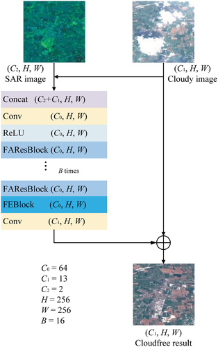
The input of FENet consists of a cloud-covered Sentinel-2 optical image and a Sentinel-1 SAR image. The input is first concatenated and then operated by a convolutional layer. Next, the feature map is activated by the Rectified Linear Unit (ReLU) activation. After this step, the Feature Aggregation Residual blocks (FAResblock) and Feature Enhancement Block (FEBlock) jointly process the features while capturing and refining both the local spatial context and global dependencies. As the last step, a convolutional layer reshapes the obtained features to match the number of spectral bands of the optical image and adds them to the original optical image. In this way, the network is able to learn and predict a residual feature map. Inside FENet, the loss function proposed in (Meraner et al. 2020) is used that compares original unclouded information in the resulting images and generates seamless and robust spectral consistency.

FENet is an end-to-end missing information reconstruction network. The cloud and cloud shadow (cloud/shadow) detection are executed and the cloud/shadow mask is obtained in the network.

2.2. FAResblock

FAResblocks are at the main body of FENet. Each FAResblock consists of six layers, five of them being the skipped layers and one of them being an addition layer (identified as $\oplus$) for the residual connection (Figure 2). This connection enables the network to learn an additive correction that eliminates the thin cloud. The five skipped layers are a convolution layer, a ReLU activation, a second convolution layer, a designed Feature Aggregation Module (FAM), and a residual scaling layer. The residual scaling layer multiplies the input feature map by a scaling factor so that the training process of the network is stabilized without bringing extra arguments.

Figure 2. The designed feature Aggregation Module (FAM), feature Aggregation residual blocks (FAResblock) and feature Enhancement block(FEBlock). FAM and LAM signify feature Aggregation Module and linear attention mechanism separately.

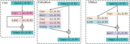
A Feature Aggregation Module (FAM) is included to avoid the possible decrease in the information reconstruction accuracy. It guarantees the accuracy of the residual blocks while maintaining lower computational complexity with a lower value of $C_0$. Figure 2 shows the structure of the FAM: it includes a convolution layer, a Linear Attention Mechanism (LAM), and a final residual layer. Both convolution layers extract the local context and employ the attention mechanism to extract the non-local context. Since the dot-product attention mechanism often adopts the softmax function (Bridle 1989) as the normalization function, resulting in $\mathit{O}\left(N^2\right)$ time and memory complexity, both memory and computational demands of the dot-attention mechanism increase quadratically with the input size. To apply the attention mechanism in the cloud removal area, we include a linear attention mechanism (LAM) as a simplified dot-product attention mechanism in FENet. It uses the first-order Taylor expansion of the softmax function (Li et al. 2021), with the complexity of $\mathit{O}\left(\mathit{N}\right)$. Hence, the efficiency of FENet is reconciled without reducing the cloud removal accuracy.

The number of channels of the output feature of this block is set to $C_0$ = 64 rather than to $C_0$ = 256 in the benchmark DSen2-CR described below (Meraner et al. 2020), in order to reduce the computational requirements and time consumption. We set B = 16 as the number of the FAResblocks and 0.1 as the scaling factor in the scaling layer.

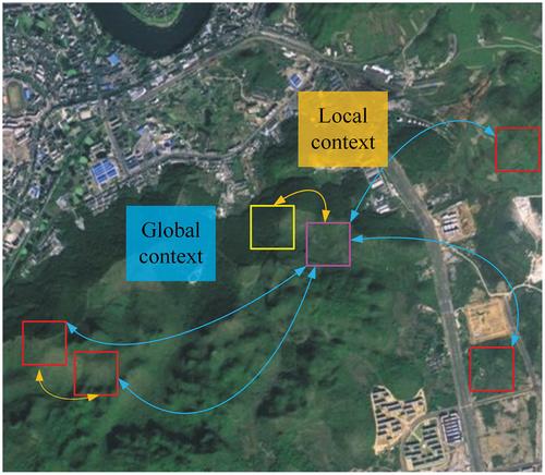
FAM compensates for a potentially degraded performance when reducing the number of channels of FAResblocks from 256 to 64. This is necessary as both the local and non-local pixels can provide cloud-covered information for the cloud-covered areas (Figure 3).

Figure 3. The global (non-local) context and local context. Pixels in the purple rectangle indicate the cloud-covered pixels, while pixels inside the yellow rectangle and red rectangle provide local and non-local context, respectively, for the cloud-covered pixels to be recovered. The squares represent the receptive view of the convolution.

2.3. Feature enhancement block (FEBlock)

As shown in Figure 2, the input of the FEBlock is processed by two branches, processing the input separately. One branch with an individual convolutional layer captures the local context information, while the other branch contains a convolutional layer and linear attention mechanism, developing the global long-range dependencies. Next, the outputs of the two branches are added and activated by ReLU, which is an activation function bringing nonlinearity into the network. The linear attention mechanism in this block is suitable for processing large datasets since it is memory-saving and computation-effective. This attention obtains the response for each pixel by measuring the similarities between the pixel pairs so that the global contextual information is extracted.

2.4. Comparison methods

In this paper, we compare FENet with the DSen2-CR benchmark (Meraner et al. 2020) and state-of-the-art GLF-CR method (Xu et al. 2022).

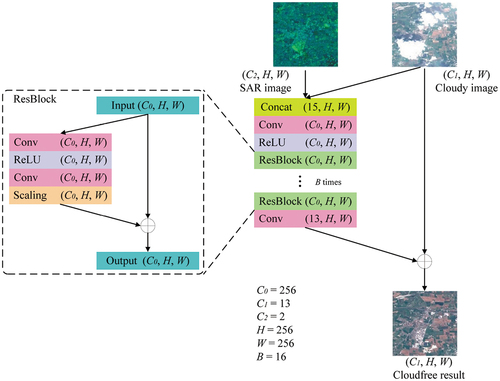
DSen2-CR method. Fig. 4 presents the diagram of the DSen2-CR network. The main body of this network consists of B = 16 residual blocks, and each block extracts a feature of $C_0,\mathit{H},\mathit{W}$ = (256, 256, 256) size, where $C_0$ indicates the number of channels, $\mathit{H}$ denotes the height and $\mathit{W}$ represents the width of the feature maps. The residual block consists of five skipped layers: a convolution layer, a ReLU activation layer, a second convolution layer, a scaling layer, and an addition layer. The output of the residual blocks is fed into a convolution layer and added to the original cloudy image. In this network, all the extracted contexts are local contexts without global contexts. As the channel numbers are high, the computational complexity and consumption are large.

Figure 4. DSen2-CR model graph.

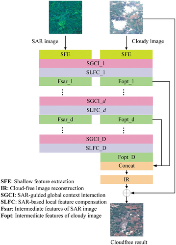
GLF-CR method. The structure of the GLF-CR network is shown in Figure 5. The core part of the GLF-CR network is $\mathit{D}$ SGCI and SLFC blocks. The SGCI block has two branches for the input and processing of optical and radar features. Inside each branch, a swin transformer block is used to extract the long-range contextual information. The SLFC first use dynamic filtering to process the speckle noise in the SAR image and then learn residual information between SAR and optical features for optical feature compensation. $\mathit{D}$ optical features produced by SLFC blocks are concatenated and processed by IR block. The cloud-free result is obtained by adding the original cloudy image and output of the IR block. For more detailed information about the structure and details of GLF-CR, please refer to the article (Xu et al. 2022).

Figure 5. GLF-CR model graph. $\mathit{D}$ indicates the number of the SGCI and SLFC blocks.

3. Experiments and results

3.1. Experimental settings

3.1.1. Dataset and metrics

For the large-scale SEN12MS-CR dataset (Ebel et al. 2020), we tested the effectiveness and efficiency of FENet. SEN12MS-CR contains 122,218 patch triplets with coregistered Sentinel-1 SAR data as well as cloud-covered and cloud-free 13-band multispectral Sentinel-2 images. The dataset covers 169 non-overlapping Regions of Interest (ROIs) uniformly distributed over all continents and meteorological seasons. The heterogeneity of the land cover in this dataset is guaranteed because the optical images are obtained in four seasons, and the surface changes are limited because the images of the three modalities were acquired in the same meteorological season. The average size of the ROIs is approximately 5,200 × 4,000 pixels, and the mean area of the ROIs is approximately 52 × 40 $\mathit{k}{m}^2$. Each scene in the dataset is stored in Universal Transverse Mercator (UTM) projection and partitioned into patches of 256 × 256 pixels. Approximately half of the optical images are impacted by clouds and the amount of coverage for different patches varies significantly (Ebel et al. 2020).

To quantitatively evaluate the results of different cloud removal methods, unitless structural similarity (SSIM) index (Wang et al. 2004), mean absolute error (MAE), the root-mean-square error (RMSE) in units of top-of-atmosphere reflectance (${\rho }_{\mathit{TOA}}$), and peak signal-to-noise ratio (PSNR) in decibel units are employed in the experiments.

In the following formulas, $\mathit{Oi},\mathit{j}$ and $\mathit{Ri},\mathit{j}$ represent the ground truth image and resulting images of reconstruction methods, respectively. The numbers of rows and columns of the image are separately denoted as m and n, and (i, j) means the pixel location in an image. The MAE and RMSE evaluate metrics for pixel-wise reconstruction quality:

(1) $\mathit{MAE}\frac{1}{\mathit{mn}}\sum _{\mathit{i}=1}^m\sum _{\mathit{j}=1}^n|\mathit{R}(\mathit{i},\mathit{j})-\mathit{O}(\mathit{i},\mathit{j})|$(1)

(2) $\mathit{RMSE}\sqrt{\frac{1}{\mathit{mn}}\sum _{\mathit{i}=1}^m\sum _{\mathit{j}=1}^n||\mathit{R}(\mathit{i},\mathit{j})-\mathit{O}(\mathit{i},\mathit{j})||{ }^2}$(2)

The PSNR refers to the rate of the possible peak pixel intensity to the power of the noise. PSNR could be derived according to Equation 3(3) $\begin{array}{c}\mathit{PSNR}10\times \mathit{lo}{g}_{10}(\frac{\mathit{MAX}}{\mathit{MSE}})\end{array}$(3) , where MAX means the possible peak value of all the pixels in the image $\mathit{Ri},\mathit{j}$.

(3) $\begin{array}{c}\mathit{PSNR}10\times \mathit{lo}{g}_{10}(\frac{\mathit{MAX}}{\mathit{MSE}})\end{array}$(3)

SSIM is a synthesis index that combines contrast, luminance, and local image structure. SSIM gets structures through neighbouring pixel intensities after normalizing the image and obtaining contrast and brightness. Compared with PSNR, the value of the SSIM index is more consistent with the visual effect because human eyes excel at capturing the structure.

(4) $\begin{array}{c}\mathit{SSIM}={\left\{\mathit{l}[\mathit{R}(\mathit{i},\mathit{j})\mathit{O}(\mathit{i},\mathit{j})]\right\}}^{\alpha }\cdot {\left\{\mathit{c}[\mathit{R}(\mathit{i},\mathit{j})\mathit{O}(\mathit{i},\mathit{j})]\right\}}^{\beta }\cdot {\left\{\mathit{s}[\mathit{R}(\mathit{i},\mathit{j})\mathit{O}(\mathit{i},\mathit{j})]\right\}}^{\gamma }\end{array}$(4)

Equation 4(4) $\begin{array}{c}\mathit{SSIM}={\left\{\mathit{l}[\mathit{R}(\mathit{i},\mathit{j})\mathit{O}(\mathit{i},\mathit{j})]\right\}}^{\alpha }\cdot {\left\{\mathit{c}[\mathit{R}(\mathit{i},\mathit{j})\mathit{O}(\mathit{i},\mathit{j})]\right\}}^{\beta }\cdot {\left\{\mathit{s}[\mathit{R}(\mathit{i},\mathit{j})\mathit{O}(\mathit{i},\mathit{j})]\right\}}^{\gamma }\end{array}$(4) shows the components of the SSIM. $\mathit{lRi},\mathit{jOi},\mathit{j}$ means the luminance comparison between two images, while $\mathit{cRi},\mathit{jOi},\mathit{j}$ indicates the contrast and $\mathit{sRi},\mathit{jOi},\mathit{j}$ implies the structure comparison. α, β, γ are the weights of these three components in SSIM. The specific methods for these three components can be referred in (Wang et al. 2004).

3.1.2. Implementation details

The proposed FENet and the benchmark DSen2-CR method are implemented using Python programming language and PyTorch deep learning framework. The GLF-CR network is implemented using C and Python programming languages. The networks are trained using two NVIDIA 2080ti with Adam optimizer. The learning rate is set at $7\times {10}^{-5}$. The SEN12MS-CR dataset contains 122,218 triplets and was split into training, validation, and test datasets. The test, validation, and training datasets include 5998, 6668, and 109,552 patches, respectively. The images are augmented by horizontal and vertical axis flipping. All the experiments use identical training, validation, and test datasets.

Due to the large size of the GLF-CR model, training it with the current available computational resources is not feasible. Therefore, several modifications to the default GLF-CR network settings are required. The batch size is adjusted to 1 instead of 12. Additionally, we set the number of input channels for the shallow feature extraction block to 48. In the SAR-guided global context interaction block, each stream has 4 dense connections. Moreover, the residual dense blocks are configured with 4 convolutional layers, and the output channels of the residual dense block are set to 24. The adjustments are based on the maximum capacity that our computer can handle.

Figure 6. Four example thin and partially covered cloud removal results of DSen2-CR, GLF-CR and FENet on the SEN12MS-CR dataset. (a,f,k,p) are the original cloud-covered image. (b,g,l,q) are the reconstruction results of DSen2-CR. (c,h,m,r) are the reconstruction results of GLF-CR. (d,i,n,s) are the reconstruction results of FENet. (e,j,o,t) show the reference image.

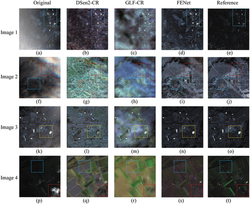
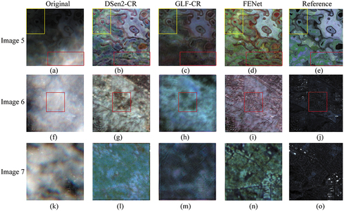
Figure 7. Three example thick and large-area covered cloud removal results of DSen2-CR, GLF-CR and FENet on the SEN12MS-CR dataset. (a,f,k) are the original cloud-covered image. (b,g,l) are the reconstruction results of DSen2-CR. (c,h,m) are the reconstruction results of GLF-CR. (d,i,n) are the reconstruction results of FENet. (e,j,o) shows the reference image.

3.2. Experimental results

3.2.1. Effectiveness of the proposed networks

Table 1 lists the accuracies of the results of FENet, GLF-CR and DSen2-CR tested on the SEN12MS-CR dataset. According to this table, FENet shows better performance than DSen2-CR and GLF-CR, as indicated by higher PSNR and SSIM values and lower MAE and RMSE values. Specifically, compared with DSen2-CR, FENet shows an increase in PSNR and SSIM values from 28.13 and 0.8651 to 28.51 and 0.8764, respectively, while the MAE and RMSE values decrease from 2.92 and 4.09 to 2.87 and 3.97, respectively. The results suggest that FENet produces higher-quality images that are more similar to the reference images. The effectiveness of the proposed FENet is evidenced by its ability to achieve high-accuracy results while utilizing fewer channels compared to the benchmark network. Additionally, FENet requires less computational resources compared to GLF-CR while obtaining higher accuracies.

Table 1. The accuracies of DSen2-CR, GLF-CR and the proposed FENet on the SEN12MS-CR dataset.

Method	PSNR	SSIM	MAE(${\rho }_{\mathit{TOA}}$)	RMSE(${\rho }_{\mathit{TOA}}$)
DSen2-CR	28.13	0.8651	2.92	4.09
GLF-CR	26.89	0.8463	3.68	4.93
FENet	28.51	0.8764	2.87	3.97

Figure 6 shows instances of cloud removal with thin and partially covered clouds, while Figure 7 depicts cases of cloud removal with thick and large-area covered clouds. The reference images shown in the figures are cloud-free Sentinel-2 satellite images obtained during the same season with the cloudy images that were recovered. Next, we evaluate the experimental result on the basis of visual effects.

In Figure 6, cloud removal of the proposed network achieves higher spectral consistency. The overall spectral signatures of FENet’s results are darker and closer to those of the reference images. Figure 6d shows that FENet has a higher capacity in preserving original cloud-free information. Specifically, the area in the blue rectangle in Figure 6d depicts more distinct building boundaries and sharp roads as compared to Figure 6b, c, where the roads and buildings appear blurred. Figure 6c reveals the presence of new patchy clouds and shadows within the original cloud-free area. These three methods employ an identical cloud detection methodology, and the cloud mask used in these two methods is the same. In the cloud removal task, the original cloud-free area contains the real reflected electromagnetic radiation information. As a result, altering this information during the cloud removal process may introduce errors. Therefore, FENet outperforms DSen2-CR and GLF-CR methods by retaining more original cloud-free information. The cloud-covered 2 in Figure 6 covers an urban area, containing a more complicated surface than 1 In Figure 6h, the area in the blue rectangle contains more clear roads and buildings than the corresponding area in Figure 6g, which agrees with the findings of the experiments on 1 in Figure 6. For the cloud-covered area, e.g. the areas in the red rectangle Figure 6f, the reconstruction result of FENet is visually more similar to the reference image and represents more complex texture and fine details. 3 in Figure 6 illustrates an example of fog removal. The result obtained by FENet in Figure 6n is more distinct than that of the result of the benchmark and the state-of-the-art methods. Image 4 presents a case of cropland covered by small thick clouds. It is noticed that the edges of roads and croplands are shadowy in the Figure 6q, r (the area in the blue rectangle), while the corresponding area in Figure 6s reveals sharp edges of the croplands and clearly visible houses. For the small thick cloud in the red rectangle in Figure 6s, FENet reconstructs the small buildings, while the vestige of the cloud still appears in the comparison methods’ result. Besides, in terms of the general spectrum, it is also evident that our results closely resemble the reference image.

In Figure 7, the recovery results are not as good as the results in Figure 6 since the clouds are thicker and have larger sizes. The recovery areas still include more and finer details with small textures, intricate patterns, and delicate lines. Figure 7 displays an image that shows a transition from thick clouds in the bottom right corner to thin and cloudless skies in the top left corner. The red and yellow rectangles indicate the thick cloud and cloudless areas, respectively. Compared with the result of DSen2-CR and GLF-CR, FENet generates a more reliable result (Figure 7d) that is consistent with the reference image (Figure 7e). Both the original cloudless and constructed thick cloudy areas of FENet’result present textures closer to the reference image. Figure 7f displays a large size thick cloud covered image. The result of FENet exhibits more details, and the complex roads in the red rectangle are more clear. Figure 7k gives an example of large size thick cloud that has different thicknesses. The cloud pattern still appears in Figure 7l, while Figure 7n reveals the roads and building complex under the clouds.

3.2.2. Efficiency of the proposed networks

In this section, we examine the efficiency of FENet. Table 2 presents the amount of parameters, complexity, and speed of DSen2-CR, GLF-CR and FENet. The ’speed’ refers to the required amount of processing time of the network to process an image in the SEN12MS-CR dataset. The ’training time’ refers to the number of hours required to train one epoch on the SEN12MS-CR dataset. The speed and the training time of GLF-CR are calculated based on the adjusted hyperparameters we set. Due to the network being partially programmed in C and partially in Python, we face challenges in accurately calculating the complexity and parameter count. Therefore, these two data are not included in the table. Table 2 shows that the complexity of FENet is only around $10\mathrm{\%}$ of that of DSen2-CR, and that FENet is capable of processing images three times faster than DSen2-CR. The method can process one image using 51 ms, while the benchmark method takes 206 ms. For FENet, less training time is required. It takes only less than 8 hours to train one epoch, reducing the training time from over 10 hours (benchmark method) to less than 8 hours. Compared to the state-of-the-art method, we reduce the training time by over 10 hours. According to the GLF-CR paper, we set the training to 30 epochs for the GLF-CR method. We employ a combination of early stopping and a maximum number of epochs to stop training for FENet. FENet is trained for a total of 43 epochs. In terms of total training time, FENet saves more than one week of time on training with the SEN12MS-CR dataset, compared with the GLF-CR method. Moreover, the amount of the parameters is reduced from 18.94 M to 1.91 M. The required computational resources are significantly reduced by the proposed FENet. This reduction allows FENet to handle large datasets more efficiently for real-world applications. Furthermore, the efficient attention mechanism maintains the efficiency of the network as well as improves the accuracies by extracting the global context.

Table 2. The efficiency of DSen2-CR, GLF-CR and FENet.

Method	Parameters(M)	Complexity(GMac)	Training time(h/epoch)	Speed(ms)
DSen2-CR	18.94	1241.48	10.047	206
GLF-CR	-	-	18.145	99
FENet	1.91	125.21	7.835	51

3.2.3. Ablation study about designed blocks

Ablation experiments are performed to evaluate the effectiveness of FAM and FEBlock in enhancing the performance of FENet for cloud removal. The baseline is FENet without the FAM and FEBlock. Table 3 shows the results of the ablation experiments. The baseline model exhibits modest accuracy due to a limited number of channels. Incorporating the designed efficient blocks improve PSNR and SSIM while reducing RMSE and MAE values. The designed FAM improves the PSNR and SSIM values from 27.91 and 0.8497 to 28.09 and 0.8629, respectively, and reduced both the MAE and RMSE values by 0.1. Furthermore, the designed FEBlock raises the PSNR (28.09 to 28.51) and SSIM (0.8629 to 0.8764) values while decreasing the MAE (3.01 to 2.87) and RMSE (4.18 to 3.97) values. These findings highlight the significance of global dependencies in cloud removal. The designed blocks extract global context by attention mechanism and use residual connections to better reconstruct missing information under both thick and thin cloud cover. The attention mechanism can identify the most relevant parts of the input for a given task, enabling FENet to focus on the most important image features. This leads to more accurate cloud removal results and improved overall performance.

Table 3. The results of the ablation experiments.

Method	PSNR	SSIM	MAE(${\rho }_{\mathit{TOA}}$)	RMSE(${\rho }_{\mathit{TOA}}$)
Baseline	27.91	0.8497	3.11	4.28
Baseline+FAM	28.09	0.8629	3.01	4.18
FENet	28.51	0.8764	2.87	3.97

3.2.4. Cloud removal results under challenging situations

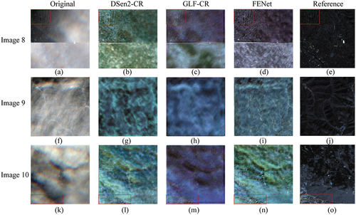
Figure 8 shows typical examples of cloud removal under challenging conditions. In practical remote sensing applications, it is common to use image division and image stitching to split large images and generate smaller and more manageable partitions that can be analysed using sophisticated algorithms. Figure 8a shows cloud removal where the cloud-covered image is generated by joining different small pieces of images. This leads to a reconstruction result containing a white line with high pixel values and the land cover is cut off here. Hence FENet at present cannot deal with the image without a perfect mosaic process in practical applications. The joined images can only be processed by removing the cloud in two different patches. As shown in the red rectangle in Figure 8b–d, FENet reserves more details in the original cloud-free image than the comparison networks. Figure 8f, k show clouds with much texture (e.g. cirrocumulus and cirrus) and varying thickness. The outline and texture of the clouds are not completely removed in the results, and the cloud pattern is slightly visible in the results of the two networks. This is caused by the great amount of clouds that limit both the global context and the local context, and the individual information source is the SAR image. The SAR image only provides two polarization modes for the 13-band optical image reconstruction, hence the reconstruction results are of a low quality. Compared with the results of the DSen2-CR and GLF-CR method, however, the results of FENet still appear closer to the reference images. For instance, compared with the results in Figure 8g, h, the trace of the cloud is less obvious in Figure 8i, while in the central part of Figure 8i, the ridge and valley are reconstructed better. Besides, the information under the thin clouds is recovered well by FENet, especially the part in the red rectangle in Figure 8n where the details are enough and the roads are clear. Even though the available global information is limited due to the presence of many clouds, the utilization of global information in FENet can help to reconstruct the information.

Figure 8. Three example cloud removal results of DSen2-CR and FENet under challenging conditions on the SEN12MS-CR dataset. (a,f,k) are the original cloud-covered image. (b,g,l) are the reconstruction results of DSen2-CR. (c,h,m) are the reconstruction results of FENet. (d,i,n) are the reconstruction results of FENet. (e,j,o) shows the reference image.

4. Discussion

This paper proposes FENet as a novel network for cloud removal in satellite images using SAR-optical image fusion. The proposed feature enhancement network decreases the computational complexity and improves the performance of the cloud removal network.

A major advantage of FENet is its ability to handle varying degrees of cloud coverage, including thin and thick clouds, which can be a challenging task for existing cloud removal methods. Compared with the benchmark and state-of-the-art method, FENet generates more visually precise results with improved quantitative metrics values. FENet is capable to remove the clouds while preserving the important features of the image. It generates clear boundaries for buildings, roads and other objects on the ground. The transition between the reconstructed region and the original cloud-free region does not show any anomalous discontinuity. Another advantage is its high computational efficiency. It requires fewer computational resources hence the network can be operated on a wide range of computing systems. Further, its high speed can free up the long waiting time of training a network in a large dataset. This is because FENet has a low complexity with efficient attention mechanisms. In particular, its attention mechanism extracts global context, which helps the network to reconstruct comprehensive details and general spectral signatures. Therefore, FENet is able to produce satisfactory cloud-free results at a relatively high speed.

The quality of the results generated by FENet might be influenced by several factors. First, the registration errors between SAR and optical images might affect the quality of the image fusion and, consequently, the cloud removal results (Zhang et al. 2021). Previous studies developed robust manual-design methods and deep learning-based methods for accurately registering SAR-optical images (Yan et al. 2023; Zhang and Zhao 2023). Second, since speckle noise can reduce the quality of SAR images, advanced filtering methods need to be applied to reduce the noise while preserving the details (Shen and Wang 2023). Third, when fusing SAR and optical images, their acquisition times should be as close as possible to minimize the differences in reflectance properties of the land use/land cover classes embedded in the investigated landscapes. Lastly, reconstructing missing information becomes extremely difficult when the cloud cover is very large, i.e. covering the entire scene. This is a challenge that all existing cloud removal methods are confronted with (Meraner et al. 2020; Xu et al. 2022).

5. Conclusion

In this paper, we present a cloud removal network, called FENet, based on SAR-optical image fusion. We designed novel blocks to extract detailed local and global context information to increase information reconstruction accuracy, and the ablation experiments prove the effectiveness of the designed blocks. Applying FENet to reconstruct cloud-covered pixels, we find that it is both effective and reliable. Compared with the benchmark method, it proves a faster method by the experimental results.

Therefore, we conclude that FENet is suitable for removing clouds in large datasets. This study further proves that the cloud removal task on a large dataset can be addressed by an efficient network. The complexity and the computational resources requirements of the method are low, and thereby the image patches can be larger to contain more cloud-free information for global information extraction when using this method. Small patches can better be processed separately rather than jointly. The experiments show that the proposed method treats monotonous and thin clouds better than complex and rough clouds (e.g. cirrocumulus). We suggest using our pre-trained model on the large global SEN12MS-CR dataset (Ebel et al. 2020) rather than training FENet from scratch. Future work may focus on the reconstruction of expansive and textured cloud-covered areas.

Disclosure statement

No potential conflict of interest was reported by the author(s).

Data availability statement

The SEN12MS-CR data used in the experiments are created by (Ebel et al. 2020) at https://doi.org/10.1016/j.isprsjprs.2020.05.013. It is openly available at https://doi.org/10.14459/2020mp1554803.

References

- Addink, E. A., and A. Stein. 1999. “A Comparison of Conventional and Geostatistical Methods to Replace Clouded Pixels in NOAA-AVHRR Images.” International Journal of Remote Sensing 20 (5): 961–977. https://doi.org/10.1080/014311699213028.
- Angel, Y., R. Houborg, and M. F. McCabe. 2019. “Reconstructing Cloud Contaminated Pixels Using Spatiotemporal Covariance Functions and Multitemporal Hyper- Spectral Imagery.” Remote Sensing 11 (10): 1145. https://doi.org/10.3390/rs11101145.
- Bocharov, D. A., D. P. Nikolaev, M. A. Pavlova, and V. A. Timofeev. 2022. “Cloud Shadows Detection and Compensation Algorithm on Multispectral Satellite Images for Agricultural Regions.” Journal of Communications Technology and Electronics 67 (6): 728–739. https://doi.org/10.1134/S1064226922060171.
- Bridle, J. 1989. “Training Stochastic Model Recognition Algorithms as Networks Can Lead to Maximum Mutual Information Estimation of Parameters.” Advances in Neural Information Processing Systems 2: 211–217.
- Cheng, Q., H. F. Shen, L. P. Zhang, Q. Q. Yuan, and C. Zeng. 2014. “Cloud Removal for Remotely Sensed Images by Similar Pixel Replacement Guided with a Spatio-Temporal MRF Model.” Isprs Journal of Photogrammetry & Remote Sensing 92:54–68. GotoISI://WOS:000337865800005. https://doi.org/10.1016/j.isprsjprs.2014.02.015.
- Chen, S. J., W. J. Zhang, Z. Li, Y. X. Wang, and B. Zhang. 2022. “Cloud Removal with SAR-Optical Data Fusion and Graph-Based Feature Aggregation Network.” Remote Sensing 14:14. Chen, Shanjing Zhang, Wenjuan Li, Zhen Wang, Yuxi Zhang, Bing 2072-4292, GotoISI://WOS:000831948400001 https://mdpi-res.com/d_attachment/remotesensing/remotesensing-14-03374/article_deploy/remotesensing-14-03374-v2.pdf?version=1657795338. https://doi.org/10.3390/rs14143374.
- Darbaghshahi, F. N., M. R. Mohammadi, and M. Soryani. 2022. “Cloud Removal in Remote Sensing Images Using Generative Adversarial Networks and SAR-To-Optical Image Translation.” IEEE Transactions on Geoscience & Remote Sensing 60:1–9. Darbaghshahi, Faramarz Naderi Mohammadi, Mohammad Reza Soryani, Mohsen; Soryani, Mohsen/T-1403- 2018 Naderi Darbaghshahi, Faramarz/0000-0002-5478-3341; Soryani, Mohsen/0000-0002- 8555-9617 1558-0644, https://ieeexplore.ieee.org/stampPDF/getPDF.jsp?tp=&arnumber=9627647&ref=.
- Duan, C., J. Pan, and L. Rui. 2020. “Thick Cloud Removal of Remote Sensing Images Using Temporal Smoothness and Sparsity Regularized Tensor Optimization.” Remote Sensing 12 (20): 3446. https://doi.org/10.3390/rs12203446.
- Ebel, P., M. Schmitt, X. X. Zhu, and Ieee. 2020. “Cloud Removal in Un Paired Sentinel-2 Imagery Using Cycle-Consistent Gan and Saroptical Data Fusion.” In IEEE International Geoscience and Remote Sensing Symposium (IGARSS), IEEE International Symposium on Geoscience and Remote Sensing IGARSS, 2065–2068. Ebel, Patrick Schmitt, Michael Zhu, Xiao Xiang 2153-6996, GotoISI://WOS:000664335302029 https://ieeexplore.ieee.org/stampPDF/getPDF.jsp?tp=&arnumber=9324060&ref=.
- Ebel, P., X. Yajin, M. Schmitt, and X. Zhu. 2022. “SEN12MS-CR-TS: A Remote Sensing Data Set for Multi-modal Multi-temporal Cloud Removal.” IEEE Transactions on Geoscience & Remote Sensing 60:1–14. arXiv preprint arXiv:2201.09613. https://doi.org/10.1109/TGRS.2022.3146246.
- Gladkova, I., M. D. Grossberg, F. Shahriar, G. Bonev, and P. Romanov. 2012. “Quantitative Restoration for MODIS Band 6 on Aqua.” IEEE Transactions on Geoscience & Remote Sensing 50 (6): 2409–2416. GotoISI://WOS:000304246500025. https://doi.org/10.1109/TGRS.2011.2173499.
- Guo, Y., W. Chen, X. Feng, Y. Zhang, L. Yingchao, C. Huang, and L. Yuan. 2021. “Temporal Unmixing-Based Cloud Removal Algorithm for Optically Complex Water Images.” International Journal of Remote Sensing 42 (12): 4415–4440. https://doi.org/10.1080/01431161.2021.1892853.
- Han, S., J. Wang, and S. Zhang. 2023. “Former-CR: A Transformer-Based Thick Cloud Removal Method with Optical and SAR Imagery.” Remote Sensing 15 (5): 1196. https://doi.org/10.3390/rs15051196.
- Hu, G., L. Xiaoyi, and D. Liang. 2015. “Thin Cloud Removal from Remote Sensing Images Using Multidirectional Dual Tree Complex Wavelet Transform and Transfer Least Square Support Vector Regression.” Journal of Applied Remote Sensing 9 (1): 095053. https://doi.org/10.1117/1.JRS.9.095053.
- King, M. D., W. P. M. Steven Platnick, S. A. Ackerman, and P. A. Hubanks. 2013. “Spatial and Temporal Distribution of Clouds Observed by MODIS Onboard the Terra and Aqua Satellites.” IEEE Transactions on Geoscience and Remote Sensing 51 (7): 3826–3852. https://doi.org/10.1109/TGRS.2012.2227333.
- Li, X. H., H. F. Shen, C. Zeng, and P. H. Wu. 2012. “Restoring Aqua Modis Band 6 by Other Spectral Bands Using Compressed Sensing Theory.” In 4th Workshop on Hyperspectral Image and Signal Processing - Evolution in Remote Sensing (WHISPERS), Workshop on Hyperspectral Image and Signal Processing. GotoISI://WOS:000345747000049.
- Li, R., S. Zheng, C. Zhang, C. Duan, S. Jianlin, L. Wang, and P. M. Atkinson. 2021. “Multiattention Network for Semantic Segmentation of Fine-Resolution Remote Sensing Images.” IEEE Transactions on Geoscience and Remote Sensing 60:1–13. https://doi.org/10.1109/TGRS.2021.3093977.
- Li, R., S. Zheng, C. Zhang, C. Duan, L. Wang, and P. M. Atkinson. 2021. “ABCNet: Attentive Bilateral Contextual Network for Efficient Semantic Segmentation of Fine-Resolution Remotely Sensed Imagery.” ISPRS Journal of Photogrammetry and Remote Sensing 181:84–98. https://doi.org/10.1016/j.isprsjprs.2021.09.005.
- Meraner, A., P. Ebel, X. Xiang Zhu, and M. Schmitt. 2020. “Cloud Removal in Sentinel-2 Imagery Using a Deep Residual Neural Network and SAR-Optical Data Fusion.” ISPRS Journal of Photogrammetry and Remote Sensing 166:333–346. https://doi.org/10.1016/j.isprsjprs.2020.05.013.
- Rocha, J., and J. A. Tenedorio. 2001. “Integrating Demographic GIS and Multisensor Remote Sensing Data in Urban Land Use/Cover Maps Assembly.” In IEEE/ISPRS Joint Work- shop on Remote Sensing and Data Fusion over Urban Areas, 46–51. GotoISI://WOS: 000175227500011.
- Rossi, R. E., J. L. Dungan, and L. R. Beck. 1994. “Kriging in the Shadows - Geo- Statistical Interpolation for Remote-Sensing.” Remote Sensing of Environment 49 (1): 32–40. GotoISI://WOS:A1994NZ54500004. https://doi.org/10.1016/0034-4257(94)90057-4.
- Scaramuzza, P., and J. Barsi. 2005. “Landsat 7 scan line corrector-off gap-filled product development.” Proceeding of Pecora 16:23–27.
- Shen, P., and C. Wang. 2023. “HoMenl: A Homogeneity Measure-Based Non- Local Filtering Framework for Detail-Enhanced (Pol)(in) SAR Image Denoising.” ISPRS Journal of Photogrammetry and Remote Sensing 197:212–227. https://doi.org/10.1016/j.isprsjprs.2023.01.026.
- Van der Meer, F. 2012. “Remote-Sensing Image Analysis and Geostatistics.” International Journal of Remote Sensing 33 (18): 5644–5676. GotoISI://WOS:000303585600002. https://doi.org/10.1080/01431161.2012.666363.
- Wang, Z., A. C. Bovik, H. R. Sheikh, and E. P. Simoncelli. 2004. “Image Quality Assessment: From Error Visibility to Structural Similarity.” IEEE Transactions on Image Processing 13 (4): 600–612. https://doi.org/10.1109/TIP.2003.819861.
- Wen, X., Z. Pan, H. Yuxin, and J. Liu. 2022. “An Effective Network Integrating Residual Learning and Channel Attention Mechanism for Thin Cloud Removal.” IEEE Geo- Science and Remote Sensing Letters 19:1–5. https://doi.org/10.1109/LGRS.2022.3161062.
- Xu, F., Y. Shi, P. Ebel, Y. Lei, G.-S. Xia, W. Yang, and X. Xiang Zhu. 2022. “GLF-CR: SAR-Enhanced Cloud Removal with Global–Local Fusion.” ISPRS Journal of Photogrammetry and Remote Sensing 192:268–278. https://doi.org/10.1016/j.isprsjprs.2022.08.002.
- Yan, X., Z. Shi, L. Pei, and Y. Zhang. 2023. “IDCF: information distribution composite feature for multi-modal image registration.” International Journal of Remote Sensing 44 (6): 1939–1975. https://doi.org/10.1080/01431161.2023.2193300.
- Yin, G., G. Mariethoz, and M. F. McCabe. 2016. “Gap-Filling of Landsat 7 Imagery Using the Direct Sampling Method.” Remote Sensing 9 (1): 12. https://doi.org/10.3390/rs9010012.
- Zhang, X., C. Leng, Y. Hong, Z. Pei, I. Cheng, and A. Basu. 2021. “Multimodal Remote Sensing Image Registration Methods and Advancements: A Survey.” Remote Sensing 13 (24): 5128. https://doi.org/10.3390/rs13245128.
- Zhang, X., Z. Qiu, C. Peng, and Y. Peng. 2022. “Removing Cloud Cover Interference from Sentinel-2 Imagery in Google Earth Engine by Fusing Sentinel-1 SAR Data with a CNN Model.” International Journal of Remote Sensing 43 (1): 132–147. https://doi.org/10.1080/01431161.2021.2012295.
- Zhang, Q., Q. Yuan, L. Jie, L. Zhiwei, H. Shen, and L. Zhang. 2020. “Thick Cloud and Cloud Shadow Removal in Multitemporal Imagery Using Progressively Spatio-Temporal Patch Group Deep Learning.” ISPRS Journal of Photogrammetry and Remote Sensing 162:148–160. https://doi.org/10.1016/j.isprsjprs.2020.02.008.
- Zhang, W., and Y. Zhao. 2023. “An Improved SIFT Algorithm for Registration Between SAR and Optical Images.” Scientific Reports 13 (1): 6346. https://doi.org/10.1038/s41598-023-33532-1.