Evaluating global vegetation products for application in heterogeneous forest-savanna landscapes

ABSTRACT

While satellite-derived global vegetation structure products are powerful and easy to use, their utility for studying spatial patterns within heterogeneous landscapes such as forest-savanna mosaics has not been extensively evaluated. We explored the application of global vegetation structure products in heterogeneous landscapes by comparing them with Airborne Laser Scanning. Specifically, we assessed the accuracy and bias of two fractional cover products, MODIS Vegetation Continuous Fields (VCF) and Hansen Global Forest Change (GFC), and one global canopy height model, Global Forest Canopy Height Model (CHM), in comparison with the same variables derived from local ALS point clouds. We found that there were limitations to all three products. MODIS VCF was less accurate than its reported accuracy by at least 3%, and GFC was 10% less accurate than MODIS VCF. While Global CHM had a similar magnitude of error to its reported product accuracy, product agreement was much lower (R² 0.19 vs. R² 0.61). We also found that the context of the analysis is important when choosing whether to use one fractional product over the other. Global products should be applied with caution in heterogeneous landscapes. Increased training and validation from these landscapes could improve the performance of these products and their utility for landscape-scale ecological research.

KEYWORDS:

• forest-savanna mosaic
• tree cover
• canopy height
• LiDAR
• estimation bias

1. Introduction

In recent decades, the application of remote sensing products in ecological research has grown. Increases in spectral, spatial, and temporal resolution of optical remote sensing datasets and the proliferation of active sensors such as light detection and ranging (LiDAR) are rapidly expanding the range of opportunities to tackle ecological and biological questions integral to the conservation of threatened ecosystems and even individual species (Turner et al. 2003). Developed from satellite imagery and spaceborne LiDAR, global vegetation structure products are powerful and easy to use, providing global estimates of vegetation characteristics such as leaf area index (Myneni, Knyazikhin, and Park 2021), normalized difference vegetation index (Didan 2021), fractional tree and vegetation cover (DiMiceli et al. 2015; Hansen et al. 2013; Sexton et al. 2013) and, more recently, global estimates of canopy height (Potapov et al. 2021) and aboveground biomass (Dubayah et al. 2022).

These derived global vegetation structure products (GVPs) are frequently used to assess deforestation, habitat fragmentation and land use change (DiMiceli et al. 2021). However, the application of GVPs extends beyond solely mapping vegetation change. For example, fractional vegetation cover products have been used to delineate biomes (Miles et al. 2006), study impacts of shifting fire regimes (Staver, Archibald, and Levin 2011), estimate climate buffering capacities of forests (Davis et al. 2019), track biodiversity loss and conservation (DiMiceli et al. 2021), as well as quantify ecosystem productivity (Liang et al. 2016), soil erosion (Borrelli et al. 2017), secondary succession (Poorter et al. 2016) and restoration potential (Bastin et al. 2019). In addition to fractional cover products, GVPs that incorporate space-borne LiDAR provide 3-dimensional estimates of vegetation structure, essential for accurately mapping forest degradation (Liang et al. 2023) and assessing carbon sequestration (Houghton, Hall, and Scott 2009).

The ecological studies cited above represent some of the most highly cited applications of GVPs, most of which use two major fractional cover products, MODIS Vegetation Continuous Fields (VCF) (DiMiceli et al. 2015) and the Global Forest Change dataset (Hansen et al. 2013). MODIS VCF collection 6 is derived from 250 m Terra MODIS satellite data. It provides a continuous record of fractional land cover for treed, non-treed, and bare landscapes dating back to the year 2000. The Global Forest Change dataset developed by Hansen et al. (2013) is derived from 30 m Landsat time-series data. The product provides fractional cover in the year 2000, as well as cover gain and loss each year through the present (2022). In addition to products that map fractional canopy cover, the Global Canopy Height Model recently developed by Potapov et al. (2021) incorporates LiDAR data. This product is derived from Global Ecosystems Dynamics Investigation (GEDI) spaceborne waveform LiDAR and 30 m Landsat data and provides a canopy height at 30 m resolution.

While GVPs are extremely valuable for analysing ecological patterns and processes at large scales, their effective application requires overcoming several challenges, including limits in spatial resolution and systematic bias in product error. Coarse resolution GVPs with pixel sizes greater than 250 m (i.e. MODIS VCF) may not be able to effectively discern ecological processes due to substantial spectral mixing (Sanchez‐Azofeifa et al. 2017). The need for increased spatial resolution is especially true in fine-scale heterogeneous landscapes (Miettinen, Stibig, and Achard 2014). For example, forest-savanna mosaics are a widespread phenomenon across tropical biomes, in which patches of structurally distinct forest and savanna form landscape-scale mosaics (Dantas et al. 2016). These mosaics may exist in patches smaller than the GVP’s 250 m resolution (Pletcher, Staver, and Schwartz 2022; Goetze, Hörsch, and Porembski 2006). Additionally, evidence shows MODIS VCF consistently underestimates tree cover in tropical savanna (Adzhar et al. 2021; Gaughan, Holdo, and Anderson 2013; Staver and Hansen 2015). Finally, GVPs rely on calibration techniques and validation data that are not distributed evenly across continental regions and biomes.

In Southeast (SE) Asia, seasonally dry tropical forest structure is complex and often characterized as a mosaic of open, grassy savanna and closed forest (Bunyavejchewin et al. 2011; Khaing et al. 2019; Hamilton, Penny, and Hall 2020; Stott 1990). SE Asian savannas are threatened by woody encroachment (Kumar et al. 2019), and the region is expected to shift towards taller evergreen trees (Scheiter et al. 2020). Accurate, high-resolution maps of tree cover could help better understand the ecological drivers of vegetation structure in this region, as well as document and predict future changes to vegetation.

Independent verification is a valuable method for understanding how global estimates of tree cover may diverge from local scale estimates (Cunningham, Cunningham, and Fagan 2019; Gross et al. 2018). Three-dimensional point clouds produced through airborne laser scanning or ALS have become a widely accepted proxy for field collected vegetation structural metrics (Coops et al. 2021; Lovell et al. 2003; Tinkham et al. 2012; White et al. 2016). ALS point clouds are particularly well suited to canopy cover and height estimates (Means et al. 2000; White et al. 2016). Due to their high level of accuracy, ALS-derived structural data have been used to evaluate the quality of other remotely sensed data products (Tompalski et al. 2021). After processing and calibration, these highly accurate ALS datasets provide an opportunity to evaluate GVP accuracy.

Here, we assess the accuracy of GVPs in mapping vegetation structure in a heterogeneous, seasonally dry tropical forest landscape in SE Asia. First, we derive two canopy structural metrics, percent canopy cover and canopy height, across the study area using ALS. Using these ALS-derived variables as a ‘verification’ dataset, we evaluate the product accuracy of several satellite products commonly used in ecological studies: MODIS Vegetation Continuous Fields (VCF) (DiMiceli et al. 2015), Global Forest Change (GFC; Hansen et al. 2013) and Global Forest Canopy Height Model (Global CHM; Potapov et al. 2021). Our main objective in evaluating these three GVPs was to assess how the accuracy in highly heterogeneous landscapes compares to that reported in the products’ accuracy assessments, and to quantify the direction and magnitude of each product’s bias. We expected that Global CHM values would be the most accurate, and close to observed ALS CHM values, with strong linear correlation. We predicted that the GFC dataset would perform better than MODIS VCF, due to its higher spatial resolution and highly heterogeneous nature of the landscape. These results have the potential to inform future research conducted in seasonally dry tropical forest and provide insight for which GVPs might be best suited for a particular study, given the context of the ecological processes under study.

2. Materials and methods

2.1. Study region

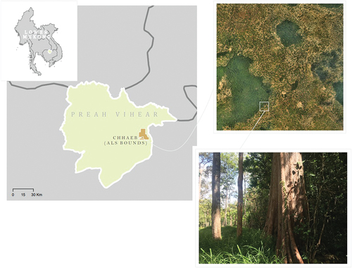
This study took place within Preah Vihear Province, Cambodia, across a 164 km² area (Figure 1). The study area sits at ~130 m above sea level and has relatively flat topography. Climatically, the region receives ~2,100 mm of rainfall per year, which is highly seasonal: during the wet season, the region receives an average of 2000 mm rainfall (May through October), while the dry season experiences less than 200 mm (November through April) (Funk et al. 2015). The study area is dominated by two forest types that differ in structure, function, and leaf habit: (1) deciduous dipterocarp forest, which is characterized by open canopy and grassy dominated understory and (2) dry evergreen forest, which is characterized by a closed canopy. Deciduous dipterocarp forest and dry evergreen forest form distinct boundaries with each other, often existing within landscape-scale mosaics (Figure 1, Fig. S1). A portion of the study area is cultivated. We include these cultivated areas in the model to test each GVP’s ability to identify areas with fragmented canopy cover.

Figure 1. Map of the study region. LiDAR data were acquired near Chhaeb, within the Preah Vihear Province of Cambodia. Seasonally dry forests extend across much of the landscape in Northern Cambodia and are composed of two distinct vegetation formations: dry evergreen forest and deciduous dipterocarp forest. Here, dry evergreen forest forms stark boundaries with deciduous dipterocarp forest, which are visible in both aerial and ground photography.

2.2. Global vegetation structure datasets

The MODIS Vegetation Continuous Fields product represents annual fractional vegetation cover for three land classes, tree cover, non-tree cover, and non-vegetated ground, at 250 m resolution. It is produced using the seven available bands, from multi-day composites of Terra MODIS (DiMiceli et al. 2015, 2021). Here, we extract and evaluate the tree cover class (percent tree cover) only. MODIS VCF tree cover has been validated against field collected canopy cover, high-resolution aerial imagery (e.g. Quickbird; Montesano et al. 2009) and GEDI L2B products (DiMiceli et al. 2021).

Hansen Global Forest Change, henceforth GFC, is a medium resolution (30 m) map of global tree cover in the year 2000 and provides annual estimates of tree cover loss and gain since year 2000. This map is the result of a time-series analysis of Landsat images, in which tree cover is defined as canopy closure for all vegetation taller than 5 m in height (Hansen et al. 2013). Additionally, this dataset uses global MODIS VCF percent tree cover as training data in development (DiMiceli et al. 2021; Hansen et al. 2003, 2013). Validation of tree cover loss and gain is provided by Hansen et al. (2013) using probability-based stratified random sampling by biome (e.g. boreal forest, temperate forest, humid tropical forest and dry tropical forest), in which reference data was collected from image interpretation of time-series Landsat, MODIS, and very high spatial imagery from Google Earth. Additionally, forest change was evaluated using satellite-collected LiDAR data from NASA’s Geoscience Laser Altimetry System instrument on board the IceSat-1 satellite (Hansen et al. 2013).

The Global Forest Canopy Height Model developed by Potapov et al. (2021), henceforth Global CHM, was created by integrating canopy structural metrics gathered from Global Ecosystem Dynamics Investigation (GEDI) with Landsat time-series. Specifically, relative height metrics for the 95^th percentile of the GEDI wave form returns were used due to high correlation with ALS-derived canopy height. The number of GEDI samples within the humid tropics was affected by cloud cover, and these areas had roughly half as many GEDI samples per unit area, compared to sub-tropical, and temperate locations. ALS validation data were collected from forests in the U.S.A., Mexico, DRC and Australia. ALS point clouds were aggregated into 30 m × 30 m grid cells based off the 90^th percentile of Z values (point height) and used in model calibration. While the calibration data set does represent a diverse set of forest types, it does not include heterogeneous landscapes, such as those that occur along forest – savanna transition zones (Bond and Parr 2010; Das et al. 2015; Fair, Anand, and Bauch 2020). For further information see Potapov et al. (2021).

We accessed and processed all global vegetation structure data using Google Earth Engine (GEE) – a cloud processing platform for large-scale geospatial data. All three datasets were present in the GEE public data catalogue. For MODIS VCF and Global CHM data, we collected tree cover/height data for the years 2015 and 2019, respectively, and clipped each raster to the study region. For GFC, absolute tree cover is reported for the year 2000 and cover change in years 2001-present is reported as either a loss (with associated year of loss), ‘lossyear’, or a gain in tree cover, ‘gain’. We updated tree cover data to reflect all tree cover lost between 2000 and 2015. For all areas that lost tree cover between 2000 and 2015, we reclassified tree cover to 0%. All pixels that gained cover during this period were masked from the analysis since no fractional cover information could be collected from these areas. We exported datasets at the same extent as ALS-derived canopy cover and canopy height models and imported them into R (version 4.0.2) for analysis.

2.3. LiDAR acquisition

LiDAR was acquired by PT McElhanney Indonesia using an AS350 B2 helicopter equipped with a Leica ALS70 sensor, during April 2015 within the context of the Cambodian Archaeological Lidar Initiative (Evans 2016). Digital photos were acquired simultaneously, and GPS survey ground support was provided by Trimble R8 GNSS receivers. Flight was carried out between 900 m and 1350 m above ground with a flight speed of 80 knots. Laser scanning was conducted with a swath width of 670 m, achieving a point density of 16 points per m², with 30% overlap of data acquisition between adjoining flight lines.

2.4. Processing LiDAR data

All ALS point clouds were preprocessed by PT McElhanney Indonesia after carrying out the LiDAR acquisition. Terrascan/Terrasolid was used to classify and separate ground and non-ground returns, using a semi-supervised process. LiDAR point clouds were then processed using both LAStools (Isenburg 2020) and the lidR package in R (see below for further explanation of these methods) (Roussel 2021; Roussel et al. 2020).

2.5. ALS-derived canopy cover

We created a digital terrain map (DTM) at 1 metre resolution, which we used to normalize all non-ground returns. We then created the canopy cover model using the normalized non-ground points by calculating the ratio of Z values (point height) above a height threshold of 5 metres (to match the threshold used in GFC and MODIS VCF products) divided by the total number of Z values (above and below the threshold) and aggregated to mean values within 30 m grid cells (to match the resolution of GFC) (Tompalski et al. 2021). We created a second canopy cover model aggregated to 250 m grid cells to match MODIS VCF resolution.

2.6. ALS-derived canopy height model

We created a canopy height model using the normalized non-ground points, first aggregating based on the mean of all non-ground points within 1 m grid cells. Then, to aggregate to 30 m grid cells, we calculated the mean, 85^th percentile, 90^th percentile, 95^th percentile, maximum and standard deviation of mean height values. We used the 90^th height percentile to evaluate the Global CHM. The 90^th percentile is recognized as aligning most closely to true canopy height values, as mean values do not accurately represent the height of canopies in areas of heterogeneous or open canopies with tall trees (Potapov et al. 2021).

2.7. Statistical analyses

Because we expected the relationship between each GVP and the ALS data to be 1:1, we used linear regression to evaluate global vegetation structural data vs. ALS data. We evaluated GFC and MODIS VCF with only non-zero values (for results of an evaluation with zero values included, see Appendix S1). In these datasets, zero values represent areas of both cleared land and naturally occurring 0% tree cover (e.g. grasslands). Because a substantial portion of the study area is characterized by 0% tree cover, including these areas inflates the amount of agreement between the GVPs and ALS data. Excluding zero values allows us to evaluate how well each dataset does at distinguishing details about structure where tree cover does exist. We report R², mean error, mean absolute error and root mean square error (RMSE) – common metrics for evaluating the accuracy of remote sensing datasets (Gatziolis, Fried, and Monleon 2010; DiMiceli et al. 2021; Graham et al. 2019; Ota et al. 2015). We binned ALS cover and height values to compare each product’s relative error (GVP-ALS) across the range of size and cover classes. Additionally, we used a regional land cover map (Dwiputra, Coops, and Schwartz 2023) to compare each product’s bias in relation to the two dominant vegetation types, deciduous dipterocarp forest and dry evergreen forest.

3. Results

All GVPs deviated significantly from ALS-derived canopy cover and height models for the study region (Table 1). Importantly, the Global CHM had the weakest agreement with the ALS data (R² of 0.19), while MODIS VCF had the highest agreement (R² of 0.83). GFC was intermediate, scoring lower in accuracy than MODIS VCF both in terms of explaining less variation (R² 0.55 vs. 0.83) and a higher RMSE (22.53% vs. 12.94%) (Table 1). While the linear regression was best fit to MODIS VCF, the relationship appears to be non-linear (Figure 2a).

Figure 2. Scatterplots demonstrating the relationship between global vegetation products and ALS cover and height. For each subplot, the grey line represents the fit linear regression for all non-zero values and the bright orange line represents the 1:1 line. Subplot (a) represents ALS-derived canopy cover vs. MODIS VCF, (b) represents ALS-derived canopy height based on the 90th percentile of height values vs. Global CHM dataset and c) represents ALS-derived canopy cover vs. Hansen Global Forest Change.

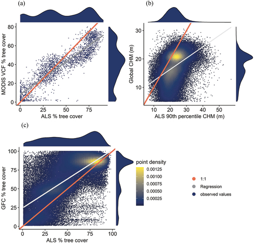
Table 1. Summary statistics for each GVP and results from evaluation with ALS-derived canopy cover and height. Mean cover and height values, linear regression equations, R², mean error, mean absolute error and RMSE are all reported.

	Mean (±sd)	Equation (x = ALS)	R^2	Mean error	Mean absolute error	RMSE
Hansen GFC	65.60% (±26.72)	GFC = 0.77× + 24.51	0.55	12.39%	17.14%	22.53%
MODIS VCF	39.74% (±20.24)	VCF = 0.69× +8.20	0.83	−5.66%	10.38%	12.94%
Global CHM	17.25 m (±4.59)	GCHM = 0.40× + 8.35	0.19	−5.14 m	5.80 m	7.27 m

Focusing on the estimation error of the fractional cover products, on average, GFC overpredicted cover by 12%, while MODIS VCF underpredicted cover by 6%. The mean canopy cover based on ALS data was 53% (±25.71) at 30 m and 45% at 250 m resolution (±26.54), whereas mean cover was 65.60% (±26.72) and 39.74% (±20.24) for GFC and MODIS VCF, respectively. The Global CHM underpredicted mean canopy height by five metres. Mean canopy height was 22.39 m (±5.10) based on the ALS data; however, the Global CHM had a mean canopy height of 17.25 m (±4.59).

3.1. The distribution of tree cover

Comparison of density plots for each data set indicated that the distribution and range of values across each dataset varied (Figure 2a–c). When the ALS-derived cover values were aggregated at 250 m, three distinct peaks formed—one at very low cover, one at intermediate cover, and one at high cover (Figure 2a). MODIS VCF, on the other hand, peaked at ~20% cover, and was noticeably missing a peak at intermediate cover (Figure 2a). Global CHM showed a multimodal distribution of canopy height, with both high and intermediate height peaks (Figure 2b), whereas ALS-derived canopy height was unimodal. Finally, the distribution of cover was similar for both GFC and ALS-derived canopy cover (Figure 2c)

3.2. The spatial distribution of bias

The seasonally dry tropical forest mosaic in the study region is made of patches of both dry evergreen forest (high tree cover) and deciduous dipterocarp forest (intermediate-to-low tree cover) (Fig. S1), and both formations are distinctly visible via aerial imagery, the ALS-derived canopy cover, and all three GVP’s (Figure 1, 3a–b). GFC’s bias was spatially aggregated based on vegetation type. While GFC overpredicted both dominate vegetation types, canopy cover tended to be more strongly overpredicted in deciduous dipterocarp forest, than within dry evergreen forest patches (Figure 3b, S2c and f). In addition to spatially aggregated bias based on vegetation type, GFC predicted low to no cover accurately in areas where land clearing was apparent (i.e. northern portion of the study area) (Fig. S3a). This pattern is also apparent in the comparison between when zero values were included in the regression analysis, and when they were not; GFC’s agreement with ALS data increased substantially when zero values were included in the regression analysis (table S1).

Figure 3. Mapped canopy cover and height for a subset of the study area. a) (clockwise from top-left) Reference orthophoto taken during ALS acquisition, classified land cover used to evaluate product performance by dominant vegetation type, ALS-derived canopy height at 30 m resolution and ALS-derived canopy cover at 30 m resolution. b) Each GVP mapped based on % cover (GFC and MODIS VCF) and height in meters (global CHM), with the respective product bias reported below.

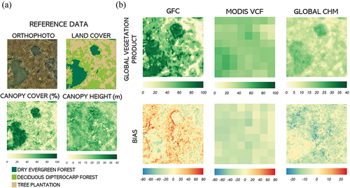
In contrast to GFC, MODIS VCF consistently underpredicts tree cover in dry evergreen forest formations and both underpredicts and overpredicts cover in deciduous dipterocarp forest (Figures. 3b and S2a and d). MODIS VCF overpredicted tree cover in areas of low-to-no cover in the northern portion of the study area (Fig. S3b), demonstrating that GFC may do better at detecting cover in highly fragmented areas than MODIS VCF. Unlike GFC, when zero values were included in the regression analysis, the level of agreement with ALS data hardly changed (table S1).

Similar to GFC, bias in global CHM was spatially aggregated based on vegetation type; deviations from ALS canopy height were most apparent within deciduous dipterocarp forest (Figures. 3b and S2b and e). The global CHM consistently underpredicted canopy height in deciduous dipterocarp forest (Figure 3b).

3.3. Further trends in deviations

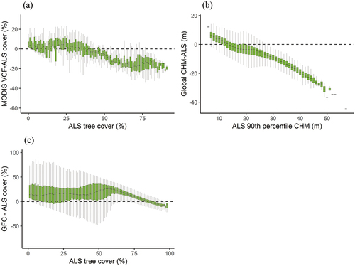
Since GFC and MODIS VCF are both models of canopy cover (as opposed to canopy height) they are directly comparable. While MODIS VCF more accurately predicted tree cover, both products were biased. The direction in which each product deviated was quite different: MODIS VCF underpredicted canopy cover by an average of 6%, while GFC overpredicted tree cover by 12% on average (mean error; Table 1, Figure 4a,c). In agreement with the results from our linear regression (Figure 2a), areas of intermediate tree cover were significantly underpredicted by MODIS VCF (Figure 4a). Divergence of GFC from ALS appears to be driven by an overall high level of noise (100% variance is common) within the model’s predictions (Figure 4c). Global CHM underpredicted height by 5 m on average, especially where canopy height was high (Table 1, Figure 4b).

Figure 4. The distribution of error for each GVP compared to the ALS-derived values of height and cover. ALS canopy cover and height are binned by whole values, and each boxplot represents the average strength and direction of bias for a given cover or height value. (a) MODIS VCF – ALS-derived canopy cover, (b) Global CHM – ALS-derived canopy height based on 90th percentile of height and (c) Hansen Global Forest Change – ALS-derived canopy cover.

4. Discussion

Here, we use ALS-derived values of canopy cover and height to evaluate GVPs’ applicability within a seasonally dry tropical forest mosaic. All three GVPs had major deviations in canopy cover and height from the observed values. MODIS VCF had the highest level of agreement based on the results of the linear regressions, yet the product consistently underpredicts intermediate tree cover typical of SE Asian seasonally dry tropical forest-savanna mosaics. GFC, does a worse job of predicting tree cover overall, with observed deviations stemming from overpredictions of canopy cover and an overall noisy dataset. Overall, Global CHM did substantially worse in predicting observed values than the cover products, underpredicting canopy height by several metres on average. Based on these results, we encourage researchers to exercise caution when applying any of these datasets to the SE Asian seasonally dry tropical forest mosaic landscape or other highly heterogeneous landscapes.

4.1. Evaluation of MODIS VCF in open canopy ecosystems

When evaluating MODIS VCF, we found higher RMSE than reported values for other regions. For example, DiMiceli et al. (2021) reported RMSE values of 9.47% and 10.4% tree cover for ground evaluation sites in Maryland and Brazil, compared to our reported value 12.94%. Our results are in agreement with other studies that demonstrate that MODIS VCF underpredicts tree cover in open canopied systems, such as savannas (Adzhar et al. 2021; Gaughan, Holdo, and Anderson 2013; Staver and Hansen 2015). Conversely, evaluation work conducted along the boreal-tundra transition zone demonstrated that the first iteration of MODIS VCF overpredicted tree cover in sparsely forested areas (Montesano et al. 2009). In general, previous research suggests that caution should be used when analysing patterns of MODIS VCF tree cover below 20–30%, a pattern which continues to persist in the most recent version (Adzhar et al. 2021; Staver and Hansen 2015). Our study further demonstrates that intermediate tree cover in heterogeneous, forest-savanna mosaics is also underpredicted in global tree cover datasets.

4.2. Evaluation of GFC and its applicability within seasonally dry tropical forest

While GFC appears to have a less consistent bias overall (error is also driven by a high level of variance), we did find that GFC exhibited a strong positive bias across the study region. This is in contrast to other research that has demonstrated that GFC tends to underpredict tree cover in seasonally dry tropical forests, especially where annual precipitation is below 2270 mm (Cunningham, Cunningham, and Fagan 2019; Fagan 2020). Our study region experiences 2100 mm rainfall/year (on the high end of rainfall typical of tropical dry forest) which may explain why we did not find that GFC underpredicted tree cover. However, other regions of SE Asia do experience less than 2,000 mm precipitation, and under-estimations of tree cover within dry tropical forest may be more prevalent within those regions.

Contrary to our predictions, we did not find higher agreement between datasets at higher resolution. Instead, the coarser resolution (MODIS VCF; 250 m resolution) performed better than GFC (30 m). This suggests that while GFC does provide a finer scale dataset to work with, it does not necessarily provide valuable additional detail on vegetation structure beyond forest loss and gain. It is important to note, however, a couple limitations to our study. First, we did not have access to field-collected validation data for the ALS-derived canopy structural metrics for our study area. Despite the demonstrated high accuracy of ALS-derived canopy measurements (Lovell et al. 2003; Tinkham et al. 2012; White et al. 2016), there could be unaccounted for bias and uncertainty in our ALS data. Second, both canopy cover products represent an annual estimate of cover, while our ALS derived cover represents late ‘leaf off’ conditions (lower than the average canopy cover), for deciduous species. This means that the positive bias exhibited by GFC may be slightly overestimated and the negative bias of MODIS VCF may be slightly underestimated. However, much of GFC’s error is driven by a high level of noise and, the lack of systematic bias in the product makes it difficult for the employment of correction techniques, as has been tested with MODIS VCF (Adzhar et al. 2021). GVP datasets utilized at global scales contain millions of data points and therefore require a large amount of computing power. As datasets increase in resolution, the number of available grid cells/data points increases rapidly. In our small study region alone, the 30 m dataset contains 165,000 grid cells vs. 3,000 grid cells in the 250 m dataset. In addition to concerns around GFC’s accuracy in comparison to MODIS VCF, researchers facing computational limitations may benefit most from MODIS VCF’s 250 m resolution. These findings suggest that while GFC may be well suited for studying fragmentation and landscape connectivity, it is less well suited for studies focused on mapping patterns of tree cover in seasonally dry tropical forest.

4.3. Limitations of global CHM

While agreement between Global CHM and ALS values was low compared to reports by the development team (R² 0.19 vs. R² 0.61, respectively), we found similar magnitudes of error, with a mean absolute error of ~6 m (Potapov et al. 2021). In developing Global CHM, ALS data was specifically collected from diverse ecosystem types in Mexico, Australia, U.S.A. and DRC, however the developers do note that their global model still underestimates canopy height within heterogeneous landscapes (Potapov et al. 2021). Given the temporal mismatch between the ALS acquisition used in this analysis (2015) and Global CHM (developed in 2019), our results may be a conservative estimation of the product’s negative bias (due to the growth and development of tree canopies). While this dataset holds promise, its use within highly heterogeneous seasonally dry tropical forests of SE Asia should be cautioned until later iterations of the product are released, which will hopefully improve based on refined and newly available GEDI observations incorporated into model calibration (Potapov et al. 2021).

Global vegetation products provide a valuable time- and cost-effective tool for scientists interested in studying ecological phenomena across regional and global scales. In this study, we demonstrate that caution should be used when applying these products to heterogeneous, forest-savanna mosaics or regions with limited calibration and validation data. In these cases, regionally specific vegetation maps may be preferred over products with global extent. Our results corroborate previous research demonstrating that MODIS VCF exhibits relatively poor agreement in regions of low to intermediate tree cover. Deciduous dipterocarp forests, with characteristically low to intermediate cover, make up one-sixth of the remaining forest in SE Asia, and tree cover within this region may be dramatically underestimated (Wohlfart, Wegmann, and Leimgruber 2014). This is especially concerning as deciduous dipterocarp forests are greatly threatened by deforestation (Sodhi et al. 2010; Wohlfart, Wegmann, and Leimgruber 2014). While 30 m resolution is ideal for assessing finer scale patterns of tree cover, we found that GFC (30 m) did not explain variation in tree cover better than MODIS VCF (250 m). This limits the applicability of using GFC to map percent cover in a complex landscape mosaic, where percent tree cover varies at fine scales. In conclusion, we encourage researchers to exercise caution when applying GVPs to highly heterogeneous landscapes, and to consider the pros and cons of each GVP, where multiple are available.

Authors’ contributions statement

EP and NBS conceived the ideas and designed methodology; DE acquired funding for and led airborne laser scanning data collection; EP analysed the data with help from SST; EP led the writing of the manuscript. All authors contributed critically to the drafts and gave final approval for publication.

Data accessibility

Global vegetation product data are freely available online from the publications cited. Airborne laser scanning data used to validate these products is available upon request.

Acknowledgements

We thank Adrian Dwiputra for helping us access the land use land classification dataset. NBS and EP received support from NSERC grant RGPIN-2019-050. The contribution of DE is funded by the European Research Council (ERC) under the European Union’s Horizon 2020 research and innovation programme (grant agreements No. 639828 and No. 866454).

Disclosure statement

No potential conflict of interest was reported by the author(s).

Supplementary Material

Supplemental data for this article can be accessed online at https://doi.org/10.1080/01431161.2023.2299278

Additional information

Funding

This work was supported by the H2020 European Research Council [639828, 866454]; Natural Sciences and Engineering Research Council of Canada [RGPIN-2019-050].

References

- Adzhar, R., D. I. Kelley, N. Dong, M. Torello Raventos, E. Veenendaal, T. R. Feldpausch, O. L. Philips, et al. 2021. “Assessing MODIS Vegetation Continuous Fields Tree Cover Product (Collection 6): Performance and Applicability in Tropical Forests and Savannas.” Biogeosciences Discussions, February, 1–20. https://doi.org/10.5194/bg-2020-460.
- Bastin, J.-F., Y. Finegold, C. Garcia, D. Mollicone, M. Rezende, D. Routh, C. M. Zohner, and T. W. Crowther. 2019. “The Global Tree Restoration Potential.” Science 365 (6448): 76–79. https://doi.org/10.1126/science.aax0848.
- Bond, W. J., and C. L. Parr. 2010. “Beyond the Forest Edge: Ecology, Diversity and Conservation of the Grassy Biomes.” Biological Conservation 143 (10): 2395–2404. https://doi.org/10.1016/j.biocon.2009.12.012.
- Borrelli, P., D. A. Robinson, L. R. Fleischer, E. Lugato, C. Ballabio, C. Alewell, K. Meusburger, et al. 2017. “An Assessment of the Global Impact of 21st Century Land Use Change on Soil Erosion.” Nature Communications 8 (1): 2013. https://doi.org/10.1038/s41467-017-02142-7.
- Bunyavejchewin S., P. J. Baker, and S. J. Davies . 2011. “Seasonally Dry Tropical Forests in Continental Southeast Asia: Structure, Composition, and Dynamics.” In In the Ecology and Conservation of Seasonally Dry Forests in Asia, edited by W. J. McShea and N. Bhumpakphan, 9–35. Washington D.C: Smithsonian Institution Scholarly Press.
- Coops, N. C., P. Tompalski, T. R. H. Goodbody, M. Queinnec, J. E. Luther, D. K. Bolton, J. C. White, M. A. Wulder, O. R. van Lier, and T. Hermosilla. 2021. “Modelling Lidar-Derived Estimates of Forest Attributes Over Space and Time: A Review of Approaches and Future Trends.” Remote Sensing of Environment 260 (July): 112477. https://doi.org/10.1016/j.rse.2021.112477.
- Cunningham, D., P. Cunningham, and M. E. Fagan. 2019. “Identifying Biases in Global Tree Cover Products: A Case Study in Costa Rica.” Forests 10 (10): 853. https://doi.org/10.3390/f10100853.
- Dantas, V. D. L., M. Hirota, R. S. Oliveira, J. G. Pausas, and M. Rejmanek. 2016. “Disturbance Maintains Alternative Biome States.” Ecology Letters 19 (1): 12–19. https://doi.org/10.1111/ele.12537.
- Das, A., H. Nagendra, M. Anand, M. Bunyan, and L. Kumar. 2015. “Topographic and Bioclimatic Determinants of the Occurrence of Forest and Grassland in Tropical Montane Forest-Grassland Mosaics of the Western Ghats, India.” PLOS ONE 10 (6): e0130566. https://doi.org/10.1371/journal.pone.0130566.
- Davis, K. T., S. Z. Dobrowski, Z. A. Holden, P. E. Higuera, and J. T. Abatzoglou. 2019. “Microclimatic Buffering in Forests of the Future: The Role of Local Water Balance.” Ecography 42 (1): 1–11. https://doi.org/10.1111/ecog.03836.
- Didan, K. 2021. MODIS/Terra Vegetation Indices 16-Day L3 Global 250m SIN Grid V061. NASA EOSDIS Land Processes DAAC. https://doi.org/10.5067/MODIS/MOD13Q1.061.
- DiMiceli, C., M. Carroll, R. Sohlberg, D.-H. Kim, M. Kelly, and J. Townshend. 2015. MOD44B MODIS/Terra Vegetation Continuous Fields Yearly L3 Global 250m SIN Grid V006. NASA EOSDIS Land Processes DAAC. https://doi.org/10.5067/MODIS/MOD44B.006.
- DiMiceli, C., J. Townshend, M. Carroll, and R. Sohlberg. 2021. “Evolution of the Representation of Global Vegetation by Vegetation Continuous Fields.” Remote Sensing of Environment 254 (March): 112271. https://doi.org/10.1016/j.rse.2020.112271.
- Dubayah, R. O., J. Armston, J. R. Kellner, L. Duncanson, S. P. Healey, P. L. Patterson, S. Hancock, et al. 2022 March. “GEDI L4A Footprint Level Aboveground Biomass Density, Version 2.1.” Ornl Drac. https://doi.org/10.3334/ORNLDAAC/2056.
- Dwiputra, A., N. C. Coops, and N. B. Schwartz. 2023. “GEDI Waveform Metrics in Vegetation Mapping—A Case Study from a Heterogeneous Tropical Forest Landscape.” Environmental Research Letters 18 (1): 015007. https://doi.org/10.1088/1748-9326/acad8d.
- Evans, D. 2016. “Airborne Laser Scanning as a Method for Exploring Long-Term Socio-Ecological Dynamics in Cambodia.” Journal of Archaeological Science 74 (October): 164–175. https://doi.org/10.1016/j.jas.2016.05.009.
- Fagan, M. E. 2020. “A Lesson Unlearned? Underestimating Tree Cover in Drylands Biases Global Restoration Maps.” Global Change Biology 26 (9): 4679–4690. https://doi.org/10.1111/gcb.15187.
- Fair, K. R., M. Anand, and C. T. Bauch. 2020. “Spatial Structure in Protected Forest-Grassland Mosaics: Exploring Futures Under Climate Change.” Global Change Biology 26 (11): 6097–6115. https://doi.org/10.1111/gcb.15288.
- Funk, C., P. Peterson, M. Landsfeld, D. Pedreros, J. Verdin, S. Shukla, G. Husak, et al. 2015. “The Climate Hazards Infrared Precipitation with Stations—A New Environmental Record for Monitoring Extremes.” Scientific Data 2 (1): 150066. https://doi.org/10.1038/sdata.2015.66.
- Gatziolis, D., J. S. Fried, and V. S. Monleon. 2010. “Challenges to Estimating Tree Height via LiDar in Closed-Canopy Forests: A Parable from Western Oregon.” Forest Science 56 (2): 139–155. https://doi.org/10.1093/forestscience/56.2.139.
- Gaughan, A. E., R. M. Holdo, and T. M. Anderson. 2013. “Using Short-Term MODIS Time-Series to Quantify Tree Cover in a Highly Heterogeneous African Savanna.” International Journal of Remote Sensing 34 (19): 6865–6882. https://doi.org/10.1080/01431161.2013.810352.
- Goetze, D., B. Hörsch, and S. Porembski. 2006. “Dynamics of Forest–Savanna Mosaics in North-Eastern Ivory Coast from 1954 to 2002.” Journal of Biogeography 33 (4): 653–664. https://doi.org/10.1111/j.1365-2699.2005.01312.x.
- Graham, A., N. C. Coops, M. Wilcox, and A. Plowright. 2019. “Evaluation of Ground Surface Models Derived from Unmanned Aerial Systems with Digital Aerial Photogrammetry in a Disturbed Conifer Forest.” Remote Sensing 11 (1): 84. https://doi.org/10.3390/rs11010084.
- Gross, D., F. Achard, G. Dubois, A. Brink, H. H. T. Prins, D. Rocchini, and M. Disney. 2018. “Uncertainties in Tree Cover Maps of Sub-Saharan Africa and Their Implications for Measuring Progress Towards CBD Aichi Targets.” Remote Sensing in Ecology and Conservation 4 (2): 94–112. https://doi.org/10.1002/rse2.52.
- Hamilton, R., D. Penny, and T. L. Hall. 2020. “Forest, Fire & Monsoon: Investigating the Long-Term Threshold Dynamics of South-East Asia’s Seasonally Dry Tropical Forests.” Quaternary Science Reviews 238 (June): 106334. https://doi.org/10.1016/j.quascirev.2020.106334.
- Hansen, M. C., R. S. DeFries, J. R. G. Townshend, M. Carroll, C. Dimiceli, and R. A. Sohlberg. 2003. “Global Percent Tree Cover at a Spatial Resolution of 500 Meters: First Results of the MODIS Vegetation Continuous Fields Algorithm.” Earth Interactions 7 (10): 1–15. https://doi.org/10.1175/1087-3562(2003)007<0001:GPTCAA>2.0.CO;2.
- Hansen, M. C., P. V. Potapov, R. Moore, M. Hancher, S. A. Turubanova, A. Tyukavina, D. Thau, et al. 2013. “High-Resolution Global Maps of 21st-Century Forest Cover Change.” Science 342 (6160): 850–853. https://doi.org/10.1126/science.1244693.
- Houghton, R. A., F. Hall, and J. G. Scott. 2009. “Importance of Biomass in the Global Carbon Cycle.” Journal of Geophysical Research: Biogeosciences 114 (G2). https://doi.org/10.1029/2009JG000935.
- Isenburg, M. 2020. LAStools—Efficient Tools for LiDar Processing (Version 200216, Academic).
- Khaing, T. T., B. O. Pasion, R. Sedricke Lapuz, and K. W. Tomlinson. 2019. “Determinants of Composition, Diversity and Structure in a Seasonally Dry Forest in Myanmar.” Global Ecology and Conservation 19 (July): e00669. https://doi.org/10.1016/j.gecco.2019.e00669.
- Kumar, D., M. Pfeiffer, C. Gaillard, L. Langan, C. Martens, and S. Scheiter. 2019. “Misinterpretation of Asian Savannas as Degraded Forest Can Mislead Management and Conservation Policy Under Climate Change.” Biological Conservation 241:108293. November, 108293. https://doi.org/10.1016/j.biocon.2019.108293.
- Liang, J., T. W. Crowther, N. Picard, S. Wiser, M. Zhou, G. Alberti, E.-D. Schulze, et al. 2016. “Positive Biodiversity-Productivity Relationship Predominant in Global Forests.” Science 354 (6309). https://doi.org/10.1126/science.aaf8957.
- Liang, M., L. Duncanson, J. A. Silva, and F. Sedano. 2023. “Quantifying Aboveground Biomass Dynamics from Charcoal Degradation in Mozambique Using GEDI Lidar and Landsat.” Remote Sensing of Environment 284 (January): 113367. https://doi.org/10.1016/j.rse.2022.113367.
- Lovell, J. L., D. L. B. Jupp, D. S. Culvenor, and N. C. Coops. 2003. “Using Airborne and Ground-Based Ranging Lidar to Measure Canopy Structure in Australian Forests.” Canadian Journal of Remote Sensing 29 (5): 607–622. https://doi.org/10.5589/m03-026.
- Means, J. E., S. A. Acker, B. J. Fitt, M. Renslow, L. Emerson, and C. J. Hendrix. 2000. “Predicting Forest Stand Characteristics with Airborne Scanning Lidar.” PE&Rs, Photogrammetric Engineering & Remote Sensing 66 (11): 1367–1371.
- Miettinen, J., H.-J. Stibig, and F. Achard. 2014. “Remote Sensing of Forest Degradation in Southeast Asia—Aiming for a Regional View Through 5–30 M Satellite Data.” Global Ecology and Conservation 2 (December): 24–36. https://doi.org/10.1016/j.gecco.2014.07.007.
- Miles, L., A. C. Newton, R. S. DeFries, C. Ravilious, I. May, S. Blyth, V. Kapos, and J. E. Gordon. 2006. “A Global Overview of the Conservation Status of Tropical Dry Forests.” Journal of Biogeography 33 (3): 491–505. https://doi.org/10.1111/j.1365-2699.2005.01424.x.
- Montesano, P. M., R. Nelson, G. Sun, H. Margolis, A. Kerber, and K. J. Ranson. 2009. “MODIS Tree Cover Validation for the Circumpolar Taiga–Tundra Transition Zone.” Remote Sensing of Environment 113 (10): 2130–2141. https://doi.org/10.1016/j.rse.2009.05.021.
- Myneni, R., Y. Knyazikhin, and T. Park. 2021. MODIS/Terra+aqua Leaf Area Index/FPAR 8-Day L4 Global 500m SIN Grid V061. NASA EOSDIS Land Processes DAAC. https://doi.org/10.5067/MODIS/MCD15A2H.061.
- Ota, T., M. Ogawa, K. Shimizu, T. Kajisa, N. Mizoue, S. Yoshida, G. Takao, et al. 2015. “Aboveground Biomass Estimation Using Structure from Motion Approach with Aerial Photographs in a Seasonal Tropical Forest.” Forests 6 (11): 3882–3898. https://doi.org/10.3390/f6113882.
- Pletcher, E., C. Staver, and N. B. Schwartz. 2022. “The Environmental Drivers of Tree Cover and Forest–Savanna Mosaics in Southeast Asia.” Ecography 2022 (8): e06280. https://doi.org/10.1111/ecog.06280.
- Poorter, L., T. M. A. Frans Bongers, A. M. Almeyda Zambrano, P. Balvanera, J. M. Becknell, V. Boukili, V. Boukili, et al. 2016. “Biomass Resilience of Neotropical Secondary Forests.” Nature 530 (7589): 211–214. https://doi.org/10.1038/nature16512.
- Potapov, P., L. Xinyuan, A. Hernandez-Serna, A. Tyukavina, M. C. Hansen, A. Kommareddy, A. Pickens, et al. 2021. “Mapping Global Forest Canopy Height Through Integration of GEDI and Landsat Data.” Remote Sensing of Environment 253 (February): 112165. https://doi.org/10.1016/j.rse.2020.112165.
- Roussel, J.-R. 2021. “Airborne LiDar Data Manipulation and Visualization for Forestry Applications [R Package lidR Version 3.1.2].” Comprehensive R Archive Network (CRAN). AccessedMarch 16, 2021. https://CRAN.R-project.org/package=lidR.
- Roussel, J.-R., D. Auty, N. C. Coops, P. Tompalski, T. R. H. Goodbody, A. Sánchez Meador, J.-F. Bourdon, F. de Boissieu, and A. Achim. 2020. “lidR: An R Package for Analysis of Airborne Laser Scanning (ALS) Data.” Remote Sensing of Environment 251 (December): 112061. https://doi.org/10.1016/j.rse.2020.112061.
- Sanchez‐Azofeifa, A., J. Antonio Guzmán, C. A. Campos, S. Castro, V. Garcia‐Millan, J. Nightingale, and C. Rankine. 2017. “Twenty-First Century Remote Sensing Technologies are Revolutionizing the Study of Tropical Forests.” Biotropica 49 (5): 604–619. https://doi.org/10.1111/btp.12454.
- Scheiter, S., D. Kumar, R. T. Corlett, C. Gaillard, L. Langan, R. Sedricke Lapuz, C. Martens, M. Pfeiffer, and K. W. Tomlinson. 2020. “Climate Change Promotes Transitions to Tall Evergreen Vegetation in Tropical Asia.” Global Change Biology 26 (9): 5106–5124. July, gcb.15217. https://doi.org/10.1111/gcb.15217.
- Sexton, J. O., X.-P. Song, M. Feng, P. Noojipady, A. Anand, C. Huang, D.-H. Kim, et al. 2013. “Global, 30-M Resolution Continuous Fields of Tree Cover: Landsat-Based Rescaling of MODIS Vegetation Continuous Fields with Lidar-Based Estimates of Error.” International Journal of Digital Earth 6 (5): 427–448. https://doi.org/10.1080/17538947.2013.786146.
- Sodhi, N. S., M. R. C. Posa, T. Ming Lee, D. Bickford, L. Pin Koh, and B. W. Brook. 2010. “The State and Conservation of Southeast Asian Biodiversity.” Biodiversity and Conservation 19 (2): 317–328. https://doi.org/10.1007/s10531-009-9607-5.
- Staver, C., S. Archibald, and S. A. Levin. 2011. “The Global Extent and Determinants of Savanna and Forest as Alternative Biome States.” Science 334 (6053): 230–232. https://doi.org/10.1126/science.1210465.
- Staver, A. C., and M. C. Hansen. 2015. “Analysis of Stable States in Global Savannas: Is the CART Pulling the Horse? – a Comment.” Global Ecology and Biogeography 24 (8): 985–987. https://doi.org/10.1111/geb.12285.
- Stott, P. 1990. “Stability and Stress in the Savanna Forests of Mainland South-East Asia.” Journal of Biogeography 17 (4/5): 373. https://doi.org/10.2307/2845366.
- Tinkham, W. T., A. M. S. Smith, C. Hoffman, A. T. Hudak, M. J. Falkowski, M. E. Swanson, and P. E. Gessler. 2012. “Investigating the Influence of LiDar Ground Surface Errors on the Utility of Derived Forest Inventories.” Canadian Journal of Forest Research 42 (3): 413–422. https://doi.org/10.1139/x11-193.
- Tompalski, P., J. C. White, N. C. Coops, M. A. Wulder, A. Leboeuf, I. Sinclair, C. R. Butson, and M.-O. Lemonde. 2021. “Quantifying the Precision of Forest Stand Height and Canopy Cover Estimates Derived from Air Photo Interpretation.” Forestry: An International Journal of Forest Research 94 (5): 611–629, May. https://doi.org/10.1093/forestry/cpab022.
- Turner, W., S. Spector, N. Gardiner, M. Fladeland, E. Sterling, and M. Steininger. 2003. “Remote Sensing for Biodiversity Science and Conservation.” Trends in Ecology & Evolution 18 (6): 306–314. https://doi.org/10.1016/S0169-5347(03)00070-3.
- White, J. C., N. C. Coops, M. A. Wulder, M. Vastaranta, T. Hilker, and P. Tompalski. 2016. “Remote Sensing Technologies for Enhancing Forest Inventories: A Review.” Canadian Journal of Remote Sensing 42 (5): 619–641. https://doi.org/10.1080/07038992.2016.1207484.
- Wohlfart, C., M. Wegmann, and P. Leimgruber. 2014. “Mapping Threatened Dry Deciduous Dipterocarp Forest in South-East Asia for Conservation Management.” Tropical Conservation Science 7 (4): 597–613. https://doi.org/10.1177/194008291400700402.