Fine-resolution land cover mapping over large and mountainous areas for Lāna‘i, Hawaii using posterior probabilities, and expert knowledge

ABSTRACT

The task of accurately mapping species-specific vegetation cover in remote and topographically complex regions like those found in Hawaiʻi presents unique challenges. This study leverages a machine learning approach to accurately classify vegetation into fine species-specific classes across the island of Lāna‘i, Hawaii, offering a novel methodology for tackling such challenges. Utilizing high-resolution WordView-2 satellite imagery, a neural network classifier and a custom lidar-based geometric correction, we introduced two new approaches to refine our high-resolution land cover classifications. This included the implementation of prior-based adjustments to class posterior probabilities to enhance land cover classification accuracy. Moreover, we developed mixed hierarchical classification maps that use class posterior probabilities to identify, at the pixel level, the finest land cover class that meets a user-defined confidence threshold. The resulting high-resolution land cover map for Lāna‘i captures the rich diversity and distribution of native and invasive plant species with high overall accuracy, generally exceeding 95%, based on independent ground control data. The capacity to produce wall-to-wall species-level vegetation maps provides a new window into monitoring vegetation dynamics on Lāna‘i and similarly remote and topographically complex regions, and contributes to our broader understanding of ecosystem responses to invasive species, climatic changes, and land management practices such as erosion and sediment control planning. Our approach offers a blueprint for similar efforts in other complex and remote ecosystems.

1. Introduction

High-resolution, accurate vegetation mapping that describes subtle differences in local, often species-specific, vegetation distribution can help support effective conservation and restoration efforts worldwide. Such mapping is necessary to monitor landscape changes, develop adaptive management strategies, and provide valuable information for land managers, researchers, policymakers, and the general public (Besnard et al. 2015; Bobbe et al. 2001; Dias, Elias, and Nunes 2004). For much of Hawaii, accurate and fine-scale land cover information has not been available to help inform conservation efforts.

Especially in regions of topographic and ecological complexity like Hawaii, a trade-off often becomes apparent between the resolution/detail and extent of classifications for land cover mapping (Fassnacht et al. 2016). On one side of this trade off, satellite-based wide-extent maps such as global and national level land cover products either generally perform poorly in these distinct and isolated systems (De Keersmaecker et al. 2021; Jung et al. 2020) or have land cover classes incompatible with commonly recognized local vegetation (e.g., ‘ōhi’a lehua (Metrosideros polymorpha) native forest) (Dinerstein et al. 2017; Olson et al. 2001). Mapping species using satellite imagery is often limited by resolution that is usually one to two orders of magnitude coarser than airborne imagery. Hawaii-specific land cover maps are available, but only at coarse resolutions and with known accuracy issues regarding class distributions. The most commonly used dataset for the state is the Hawaii GAP Analysis (HIGAP) vegetation map (Jacobi et al. 2017; McKerrow et al. 2014), which provides a comprehensive classification of native and non-native vegetation types. Another dataset that is available for Hawaii is the LANDFIRE Existing Vegetation Type (EVT) map (Rollins 2009), which was developed as part of a national programme to support fire management planning. However, both land cover products have a coarse resolution of 30 m, not sufficient to capture the spatial heterogeneity and complexity of Hawaiian ecosystems at finer scales (such as <10 m). New machine learning methods such as random forest and support vector machine applied to recently available high-resolution satellite data (e.g., WorldView-2 and 3) have shown the potential for detailed species-level mapping but often have been applied to only a subset of test species (Ferreira et al. 2019; Koerner, Chadwick, and Tebbs 2022; Vaglio Laurin et al. 2016).

On the other side of this trade off, fine-scale vegetation mapping based on airborne sensors has yielded good results but often at limited spatial extents. In Hawai‘i, coconut palms (Cocos nucifera) have been mapped on O‘ahu (Q. Chen and Lee 2020) and recent studies on Island of Hawaii have demonstrated that wall-to-wall species cover maps are feasible using airborne lidar and spectral data with high accuracy and detail; however, these studies have only been conducted at small local scales (Balzotti et al. 2020; Feret and Asner 2013). While these studies demonstrate the feasibility of high-resolution, species-level mapping for ecologically and topographically complex regions, they have relied on airborne data, which is costly and less widely available than satellite imagery.

The challenges and tradeoffs faced in accurately mapping fine-scale vegetation cover in remote and complex ecosystems are not unique to Hawaii but are representative of broader issues in remote sensing globally. This study addresses these challenges and tradeoffs by integrating and developing novel approaches for detailed and fine-resolution vegetation mapping in the island of Lāna‘i, which can be applied to other similar regions with limited relevant global datasets.

In recent years, new high-resolution satellite imagery such as WorldView-2, WorldView-3 and Sentinel-2, has become available for fine-scale land cover classification. However, their application has been limited due to factors such as data availability, return interval constraints, and large georectification issues arising from steep topography present across the Hawaiian Islands. Most commercial georectification processes rely on global digital elevation models (DEMs) with resolutions coarser than 10 m, which can result in substantial positional errors between imagery and ground truth data over topographically complex areas. To address this issue, we developed a custom geometric correction method based on the integration of independently collected light detection and ranging (lidar) datasets. This approach allows for improved alignment of high-resolution satellite imagery with ground truth data, enhancing the accuracy of vegetation mapping in regions with steep and complex terrain.

Beyond georectification issues that have limited the use of newer high-resolution satellite data for Hawaiian studies, available land cover classification products for Hawaii are several years old and still primarily rely on classical parametric classification methods, such as maximum likelihood classifiers, and do not leverage more recent machine learning methods that have shown promise elsewhere (Aigbokhan et al. 2022; Civco 1993). In our study, we apply cutting-edge machine learning techniques for land cover classification while developing probabilistic post-processing approaches for refining fine-resolution land cover maps. Posterior probabilities from fitted neural networks have been known to provide an estimate of land cover classifier confidence (Guerrero-Curieses, Alaiz-Rodríguez, and Cid-Sueiro 2009; Richard and Lippmann 1991; Ruck et al. 1990). In fact, posterior probabilities of class membership provide useful information about the magnitude and spatial distribution of classification uncertainty (De Bruin and Gorte 2000) and have been used to improve change detection (J. Chen et al. 2011), reduce biases in area estimation (Sales et al. 2022) and improve land cover classifications (Guerrero-Curieses, Alaiz-Rodríguez, and Cid-Sueiro 2009). While land cover classification post processing is commonly done by spatial smoothing such as spatially aggregating classifications using majority filters (Benediktsson, Palmason, and Sveinsson 2005; Pesaresi and Benediktsson 2001; Soille and Pesaresi 2002; Ton, Sticklen, and Jain 1991), others have suggested the use of class posterior probabilities as an effective means of reducing the appearance of misclassified isolated pixels (Guerrero-Curieses, Alaiz-Rodríguez, and Cid-Sueiro 2009). Others have integrated expert-interpreted data into classification workflows to improve land cover classifications (Zhang, Li, and Zhang 2016). In our research, we combine these approaches by (1) adjusting class posterior probabilities based on prior and expert knowledge, and (2) by using the adjusted posterior probabilities to generate mixed hierarchical land cover classifications that represent land cover class specificity based on posterior probabilities as a measure of classification certainty.

Lāna‘i provides an ideal setting to explore the development of better land cover approaches due to its accessibility, and tractable number of distinct plant communities and cover types (Jacobi et al. 2017). The island is large enough so that we can test the idea of large-area detailed vegetation mapping using satellite imagery. At the same time, it is not too large to collect sufficient high-quality reference data to train and test our methodology. Compared to other major islands in Hawaii, Lāna‘i is relatively accessible and has a reduced number of distinct plant communities and cover types, which makes this pilot study of island-wide detailed mapping feasible. By integrating multiple existing and novel approaches under these simpler conditions in Lāna‘i, we aim to develop methods that may serve as a basis for applications to the rest of Hawaii and other similarly complex and remote regions worldwide. Our study attempts not only to advance the science of vegetation mapping in Hawaii but also to contribute to the broader understanding of remote sensing and ecological work in other ecologically and topographically complex regions.

2. Methods

2.1. Satellite data acquisition

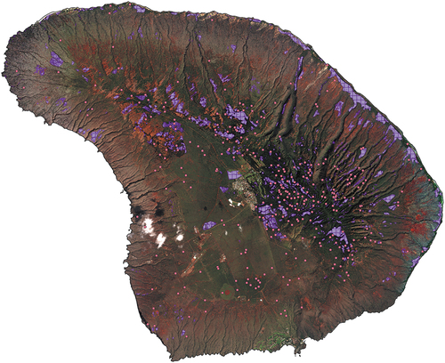
We relied on cloud-free raw/unprocessed Digital Globe WorldView-2 satellite imagery collected in February 2020 that covered nearly the entire island of Lāna‘i. This exceptionally clear dataset made us well positioned to create an up-to-date vegetation map for the island. WorldView-2 is a high-resolution satellite sensor that provides a panchromatic band (0.46 m resolution) and eight multispectral bands (1.84 m resolution); four standard colours (red, green, blue, and near-infrared 1) and four other bands (coastal, yellow, red edge, and near-infrared 2). These eight spectral bands enable enhanced spectral analysis, and related vegetation mapping.

2.2. Remote sensing data processing

Topographic complexity is one of the main challenges to create high-resolution classifications for Hawaii. Topographic complexity can cause small projection errors in fine-scale pixels over very steep terrain, leading to geopositional errors much greater than satellite image resolution. These errors can affect the accuracy and reliability of vegetation classification based on satellite imagery. For on-the-ground management applications, we found that commercially available imagery products did not have sufficient geometric accuracy, especially in steep, high elevation areas that provide habitat for several endangered animal species (e.g., Hawaiian petrel (Pterodroma sandwichensis), Partulina tree snails) and at least 10 endangered plant species including three species of hāhā (Cyanea spp.). Because of that we devised our own custom geometric correction for our raw satellite imagery utilizing airborne lidar data. We first created a digital surface model (DSM) compatible with our satellite imagery’s resolution by interpolating the lidar point cloud using the Toolbox for lidar Data Filtering and Forest Studies (Tiffs) (Q. Chen 2007). Then we orthorectified the raw WorldView-2 imagery using the ENVI Orthorectification Model for geometric correction. After geometric correction, we used ENVI and its Fast Line-of-sight Atmospheric Analysis of Spectral Hypercubes (FLAASH) atmospheric correction module to convert images from raw data to reflectance.

2.3. Vegetation class definitions

After preparing the satellite datasets for use, we met with our Lāna‘i management partners to define the management-relevant vegetation classes to be used as the focus of our analysis. This required a combination of considerations regarding not only management relevance of classes but the likely detectability of such classes from the available satellite imagery. This was an iterative process based on running preliminary vegetation classifications to identify which classes could be mapped effectively. When possible, the defined classes were species-specific, but given that some vegetation cover types across the island have multiple mixed species, some classes were more general. In the end, a total of 15 classes including all major dominant native and invasive plants were considered (Table 1). Because of the challenge to distinguish some spectrally similar species and associated classes, we generalized our original 15 species-specific vegetation classes into broader landscape classifications (or community-specific classes). This was simply done by aggregating the 15 species-specific classes into a smaller number of community-specific classes, and renaming some of the species-specific classes into more general communities they represent.

Table 1. Description of land cover class categories considered in our study.

Pixel value	Species-specific class	Class description	Community-specific class
1	Aalii native shrubland	ʻAʻaliʻi (Dodonaea viscosa) shrubland is a widespread native community on dry slopes across the island. It includes other native species as well.	Dry native shrubland
2	Albizia	Albizia (Falcataria moluccana) is an invasive tree that occurs across mid-elevation mesic slopes and can shade native species with its large, tall canopy.	Mesic mixed forest
3	Bare earth	Exposed soil. Introduced ungulates have caused massive soil degradation across the island, hence mapping and monitoring of this damage, and potential recovery is a priority.	Unvegetated
4	Brazilian pepper	Brazilian pepper (Schinus terebinthifolia) can form dense clumps in dry areas across the island and is a problematic invasive.	Dry invasive forest
5	Cook pine	Cook pine (Araucaria columnaris) was introduced across mesic high-elevation areas early last century to increase fog water capture. Stands of cook pine persist decades later.	Mesic mixed forest
6	Eucalyptus	Several Eucalyptus and other species in the myrtle family were introduced in the early 20th century to help revegetate degraded lands across the state. These now pose a threat to valuable native mesic communities as they continue to spread across the landscape.	Mesic mixed forest
7	Formosan koa	Formosan koa (Acacia confusa) can form dense stands in dry areas that leave little space for native species to grow.	Dry invasive forest
8	Ironwood	Ironwood (Casuarina sp.) stands occur in dry areas, forming dense litter beneath them where few other plants can thrive.	Dry invasive forest
9	Kiawe, Klu, and Koa haole	Kiawe (Neltuma pallida) can form dense stands in dry areas near the coast where it can access deep ground water resources. In Lāna‘i, klu (Vachellia farnesiana) and koa haole (Leucaena leucocephala) occur within these same environments and are hard to distinguish even with high-resolution imagery.	Dry invasive forest
10	Kukui	Kukui (Aleurites moluccanus), is a non-invasive tree introduced by Polynesians that has multiple uses and strong connections to Hawaiian culture.	Mesic mixed forest
11	Mixed non-native grass and shrubs	Multiple dry areas across Lāna‘i are covered by a mix of invasive grasses and invasive shrubs such as lantana (Lantana camara). These were combined into a single class since individual species differentiation from available imagery was not possible.	Dry invasive grassland
12	Non-native grassland	Non-native invasive grasslands, covering a large portion of the island’s dry environment.	Dry invasive grassland
13	Strawberry guava	Strawberry guava (Psidium cattleyanum) which is major threat to mesic and wet forests statewide and to remaining native mesic vegetation at high elevations on Lāna‘i.	Mesic mixed forest
14	Talus	Rocky areas that lack vegetation cover on the sides of the steep valleys and gorges at mid- and high- elevation across the island.	Unvegetated
15	Uluhe and Ohia	Open uluhe (Dicranopteris linearis) and ʻōhiʻa lehua (Metrosideros polymorpha) forests comprise a valuable native vegetation cover in high-elevation mesic areas. These species provide habitat for other native species, making their extent and distribution important information to guide conservation actions across multiple taxa.	Mesic native forest

2.4. Ground control data (GCD) collection

One of the essential steps for vegetation classification using machine learning methods is to collect highly accurate ground control data that can be used to train and evaluate land cover classification models. Ground control data are areas of known vegetation classes that are labelled using field observations and/or high-resolution imagery. These data provide the reference information for the machine learning algorithms to learn the spectral and spatial patterns of different vegetation types. In this study, we collected a substantial amount of ground control data for each of the defined vegetation classes described above. This involved a joint effort between the spatial analyst and Lāna‘i management staff, who spent months interpreting aerial imagery and conducting field visits to identify multiple examples for each vegetation class across the landscape. We used airborne imagery collected by EagleView, which provides ~5 cm resolution RGB colour images from multiple angles and dates.

To prepare the ground control data for machine learning, we subdivided the polygons that we delineated for each vegetation class into smaller units. This was necessary because some cover classes formed large contiguous areas across the landscape, such as Kiawe (Neltuma pallida), Klu (Vachellia farnesiana) and Koa haole (Leucaena leucocephala) class along the northern coast of the island. Using such large polygons as an input would result in too few data points not representative of within class variation for model fitting and evaluation. On the other hand, using every 2 m pixel within a polygon to represent each class would lead to issues of pseudoreplication and overfitting due to spatial autocorrelation. Therefore, we decided to use a compromise approach to balance the trade-off between sample size and spatial resolution. Hence, we segmented all polygons based on a 250 m grid that covered the entire study area. This segmentation was applied solely for dividing the large polygons (polygons greater than 10,000 m² in area) and did not involve any simplification or alteration of the vegetation classes within each grid cell. This grid size was chosen because it was coarse enough to limit overconfident classification accuracy results and reduce pseudo-replication concerns, but fine enough to capture some of the spatial heterogeneity of vegetation classes. This technique is analogous to the spatial ‘blocking’ algorithms used in training species distribution models (Valavi et al. 2019; Wenger and Olden 2012). By segmenting the original 1251 polygons, we obtained 1754 smaller polygons that represented each species-specific vegetation class at a more consistent scale (Appendix 2).

The collection of ground control data was an iterative process that involved several rounds of feedback and improvement. We first delineated initial ground control data and used them to build preliminary models using different machine learning methods. Then, our three local experts reviewed the land cover projections beyond the areas used for model fitting and evaluation and identified cover classes that could be further improved. Then we collected additional ground control data across the landscape for these land cover classes and refit the models. This process was repeated until we achieved satisfactory model performance for all vegetation classes, or no further improvements were possible based on additional ground control data collection.

2.5. Candidate land cover predictors

To train our models, we considered multiple candidate predictors that could capture the spectral and spatial characteristics of different vegetation classes. These predictors included the original WorldView2 spectral bands and several derived indices. Beyond the original eight WorldView-2 spectral bands, we calculated several spectral indices from the WorldView-2 bands using different combinations and transformations. These spectral indices are useful for enhancing certain features and enhancing land cover classifications (da Silva et al. 2020; McDonald, Gemmell, and Lewis 1998; Oon et al. 2019). We calculated brightness (a measure of overall reflectance), greenness (a measure of vegetation vigour), wetness (a measure of soil moisture), enhanced vegetation index (EVI), soil-adjusted vegetation index (SAVI), canopy chlorophyll content index (CCCI), colouration index (CoI), chlorophyll index red edge (CIrededge), normalized difference red edge (NDRE), and plant senescence reflectance index (PSNDc2). We also calculated occurrence texture indices and co-occurrence texture indices from the WorldView-2 bands using different window sizes and orientations. Texture indices are useful for describing the spatial variation or homogeneity of pixel values in an image (Haralick 1979; Haralick, Shanmugam, and Dinstein 1973). Occurrence texture indices included data range, mean, variance, entropy and skewness, while co-occurrence texture indices included mean, variance, homogeneity, contrast, dissimilarity, entropy, second moment and correlation. In addition to these predictors derived from satellite imagery data directly, we also considered some broader environmental predictors that could influence vegetation distribution and improve overall land cover classification, especially in topographically complex regions (Wang et al. 2020; Zeferino et al. 2020). These predictors were afternoon percent cloud cover (as a measure of plant water stress) at 250 m resolution; elevation, slope, and aspect at 30 m resolution. We obtained these predictors from digital elevation models and statewide climate datasets (http://climate.geography.hawaii.edu/, U.S. Geological Survey 2017) and resampled them to the same resolution as the WorldView-2 imagery using a bilinear interpolation. A total of 37 candidate predictors were calculated and considered in subsequent analyses (Appendix 1). With the GCD polygons described above, we extracted mean values for every candidate predictor variable per polygon. These mean values were then used as inputs for model training and evaluation.

2.6. Candidate predictor selection

Given the high correlation among some of our candidate predictor variables, we considered two approaches to select a reduced set of predictors from the 37 candidate variables: (1) Boruta algorithm and (2) recursive feature elimination (RFE). Boruta algorithm is a feature selection method that uses random forest models to assess the importance of each variable by comparing it with randomized copies of itself (Kursa and Rudnicki 2010). This approach aims to find all relevant features rather than a minimal optimal subset. However, the Boruta algorithm determined that 26 of the 37 variables were relevant and should be kept (listed in Appendix 1). RFE is a feature selection method that uses cross-validation to rank the importance of each variable by recursively removing the least important ones until a specified number of features is reached (Guyon et al. 2002). This approach aims to find a subset of features that maximizes model performance. RFE indicated that beyond using the top 10 predictors (listed in Appendix 1), little gains in accuracy were made in the resulting models. We fit, evaluated and projected models based on these different candidate predictor sets to pick our final model (refer to Section 2.7).

2.7. Model fitting

We used the R caret package to fit and compare four different machine learning algorithms: decision tree, random forest, naïve Bayes classifier, and a neural network model. These algorithms are widely used for classification tasks and can handle complex datasets with high dimensionality (Maxwell, Warner, and Fang 2018). Decision tree is a method that splits the data into subsets based on rules derived from the features; random forest is an ensemble method that combines multiple decision trees; a naïve Bayes classifier is a probabilistic method that assumes each feature contributes equally and independently to class probability; and neural network model is a method that uses multiple layers of neurons with interconnections defined by nonlinear functions and weights. All models were fit using only 80% of the data (training set). With that training set, the models were fit using a 10-fold cross-validation procedure, repeating the entire procedure 10 times. The resulting fitted models are an average of all these iterations and repetitions. Model accuracy was evaluated using the remaining 20% of independent data (test set). The configuration of each of the four machine learning algorithms was fine-tuned using caret’s tuning grid, which allows for optimizing hyperparameters such as number of trees, split criterion, and kernel type.

To select the best model for mapping vegetation across the island, we evaluated the performance of eight candidate models based on various combinations of the two predictor variable sets (26 predictors from Boruta feature selection algorithm and 10 predictors from RFE) and the four machine learning algorithms. We compared the models based on accuracy, class-specific sensitivities and specificities, and related confusion matrices. Based on these metrics and visual inspection of the modelled vegetation maps, we found that the neural network model based on 26 predictors and the random forest model based on 10 predictors were the two best performing models.

However, because our goal was to produce accurate land cover maps for conservation planning on Lāna‘i, we conducted a final expert review and comparison of these two models. We consulted with three experts who had a deep understanding of the landscape across the island and asked them to assess the accuracy and plausibility of each model’s vegetation classification. The experts preferred the neural network model based on the 26 candidate predictors over the random forest model based on the top 10 predictors. They determined that this model captured more nuances in vegetation patterns than the simpler model. Therefore, we selected the neural network model as our final model for mapping vegetation across Lāna‘i. This neural network model used for training had a single-hidden layer with 10 neurons (from 1 to 10 neurons considered in model tunning), logistic activation, and a decay value of 0.1 (from 0 to 0.5 considered in model tunning).

To further evaluate the accuracy of our final model, we performed an independent model accuracy evaluation using a different set of validation points than the ones used for fitting, evaluating, and comparing our models. For this evaluation, we used the final vegetation map (i.e. the neural network-based model with 26 predictors) and picked 700 randomly stratified points across the 15 vegetation classes to ensure a more equitable distribution of points across the classes considered. We then asked experts to interpret these points using their field knowledge and airborne imagery. The experts were then able to determine the actual species-specific cover class for 313 of the 700 random points and compare these assignments to the modelled classes (Figure 1). We then calculated the overall accuracies of this independent evaluation and compared them with those obtained from cross-validation. This was not only an independent accuracy assessment of the model but also a pixel-level accuracy assessment of the final vegetation map.

Figure 1. Map of collected ground control polygons segmented by a 250 m grid (purple polygons) and points used for independent validation of model results (refer to Section 2.7).

2.8. Classification refinements using class posterior probabilities and expert judgement

Based on the Bayes’ theorem (Bayes and Prince 1763), P(C|X) = P(X|C)*P(C)/P(X), where P(C|X) is the posterior probability of a pixel with a feature set of X being class C, P(X|C) is the class conditional probability that is estimated from training data, P(C) is the prior probability of a pixel being class C, and P(X) is the marginal probability of a pixel with the feature set values of X. Classification is typically implemented as a process of comparing the posterior probability P(C|X) over different classes. Because P(X) is irrelevant to any particular class, the classification problem is equivalent to comparing the product P(X|C)*P(C). In a classical supervised classification framework such as the maximum likelihood classifier, we typically assume that the prior probability P(C) is the same for different classes, so we end up simply comparing the class conditional probability P(X|C). However, we suggest that the incorporation of prior probability into the classification decision should improve the classification if we have good knowledge about the priors (Jiang et al. 2012; Shivakumar and Rajashekararadhya 2018).

Prior knowledge of the likelihood of class occurrence across geographic or environmental space can be used to adjust posterior probabilities down to reflect unlikely class occurrence (Guerrero-Curieses, Alaiz-Rodríguez, and Cid-Sueiro 2009; Zhang, Li, and Zhang 2016). These priors may be data-driven, such as being calculated as class prevalence across training samples along spatial/environmental gradients (e.g., the low prevalence of a particular class above a given reflectance value in the green satellite band); or expert-driven priors, estimated directly from expert knowledge (e.g., no expected presence of a given class away from the coast). To adjust class posterior probabilities, we tried both data- and expert-driven approaches to evaluate their pros and cons.

For the adjustment of class posterior probabilities using data-driven priors, we created prior probability rasters scaled from 0 to 1 and multiplied them by the class posterior probabilities to adjust class probabilities. The class-specific prior probability raster was created based on class prevalence (i.e. proportion of class observations from ground control data) along the range of values for variables considered. These class priors were calculated based on two different sets of variable combinations: the two principal component analysis (PCA) axes across all classification predictors and the top five predictor variables identified in the Boruta selection procedure described above. For each class and variable considered, the prior probability was calculated as the prevalence of the class along the range of values for the variable considered, based on the original ground control polygons. This prevalence was calculated by segmenting the values of the variable into four bins, as any finer binning/segmentation could result in poorly represented sections of the gradient for specific classes. The bins for each variable were defined by break points that resulted in an equivalent number of training samples across bins. For each of these class and variable prior maps, we scaled the prevalence values from 0 to 1, as without scaling rare classes would have low prior adjusted probabilities even in areas where they are most common. The prior probability raster for a given class was simply the product of the mapped scaled prevalence across all variables considered.

We also implemented expert-driven priors to adjust class posterior probabilities. This approach involved examining the prevalence of each class along environmental gradients for variables that were considered to provide good contrast among the classes of interest. Based on expert knowledge, we multiplied the class posterior probability raster by a mask that reduced the posterior probability of the class to zero for parts of a given gradient where a class was not expected exist. We applied the following expert-defined adjustments as part of our custom rule set:

1. Eucalyptus and strawberry guava (Psidium cattleyanum) posterior probabilities were adjusted to be present only where the green band value was less than 6 (where all spectral bands were scaled from 0 to 100, minimum to maximum value). This was done to help differentiate these species from native bright green uluhe (Dicranopteris linearis) vegetation.

2. Brazilian pepper (Schinus terebinthifolia) posterior probabilities were adjusted to be present only where the elevation was less than 800 m, limiting it to drier, lower elevation areas.

3. Bare soil posterior probabilities were adjusted to be present only in areas where the colouration index (CI) values were greater than 0.45.

4. Formosan koa (Acacia confusa) posterior probabilities were adjusted to be present only between 300 and 600 m in elevation.

5. Albizia (Falcataria moluccana) posterior probabilities were adjusted to be present only between 400 and 700 m in elevation, helping to differentiate it from other higher elevation mesic species.

6. Non-native grassland posterior probabilities were adjusted to be present only at elevations below 600 m, which helped to differentiate it from uluhe, the only other bright green vegetation class considered in our analysis.

7. Kukui (Aleurites moluccanus) posterior probabilities were adjusted to be present only in areas where the green band values were > 4.7 and where afternoon cloud frequency was greater than 0.7.

By applying these expert-driven adjustments, we aimed to improve the accuracy of our classification and better represent the actual distribution of the various vegetation classes across the landscape.

2.9. Mixed hierarchical land cover classification

We applied a hierarchical land cover classification approach to generate maps of different levels of detail and certainty. For each pixel, we obtained a vector of class membership probabilities for all classes considered from the classifier outputs. We then calculated the combined probabilities of coarser classes by summing the probabilities of their fine constituent classes, and then using them to produce broader maps of vegetation types. This led to a hierarchical set of land cover classification maps of increasing typological coarseness, from the original species-specific maps to coarse vegetated/unvegetated maps (Appendix 3), along with a pixel-level measure of certainty/uncertainty based on maximum class membership probabilities for each map. Finally, with the expectation that the certainty in class assignment would vary across the landscape, we created a mixed hierarchical land cover classification that integrated the multiple hierarchical land cover maps into a single map by assigning each pixel the most detailed class given a minimum class membership certainty threshold. Starting with the finest (species-specific) land cover map, pixels whose most likely class did not meet this threshold were assigned to the next coarser class until all pixels and hierarchical classes were considered. For these mixed hierarchical land cover maps we used a minimum class membership probability threshold of 0.66, equivalent to a ‘likely’ measure of certainty used by the Intergovernmental Panel on Climate Change (IPCC) (Le Treut et al. 2007), which we also found to be associated with a > 90% chance of a correct classification, based on post-model fitting analyses of the predictions for the evaluation dataset.

3. Results

Based on the 20% of the polygon ground control dataset apart for model evaluation, the overall classification accuracy across all classes was 0.962 (0.937–0.98, 95% CI). Kappa was similarly high at 0.958. Individual class accuracy was also high across all classes, never falling below 0.83 (for the Cook pine cover class; Table 2). Sensitivity (the probability of correctly identifying a true case), was also high across all classes, just dropping slightly below 0.9 for some classes (Brazilian pepper, Formosan koa, and Strawberry guava). However, the cook pine cover class had a noticeably lower sensitivity at 0.67, due to it being misclassified as other similar non-native tree cover. On the other hand, specificity (the probability of correctly identifying a negative case) was above 0.99 across all cover classes. A confusion matrix based on the evaluation data is available in Appendix 4.

Table 2. Accuracy metrics by class for the species-specific land cover classification for the island of Lāna‘i. Prevalence refers to the proportion of actual positive cases (for a particular class) across the evaluation dataset. Detection prevalence refers to the proportion of predicted positive cases (for a particular class) across the evaluation dataset. Balanced accuracy is (sensitivity+specificity)/2.

Species	Sensitivity	Specificity	Prevalence	Detection Prevalence	Balanced Accuracy
Aalii native shrubland	0.92	1.00	0.04	0.03	0.96
Albizia	1.00	1.00	0.03	0.03	1.00
Bare earth	1.00	1.00	0.12	0.13	1.00
Brazilian pepper	0.89	1.00	0.05	0.05	0.95
Cook pine	0.67	1.00	0.02	0.01	0.83
Eucalyptus	0.93	0.99	0.08	0.08	0.96
Formosan koa	0.88	1.00	0.05	0.04	0.94
Ironwood	0.98	0.99	0.12	0.12	0.98
Kiawe, kluu, and koa haole	1.00	1.00	0.19	0.19	1.00
Kukui	1.00	1.00	0.00	0.01	1.00
Mixed non-native grass and shrubs	1.00	0.99	0.06	0.07	1.00
Non-native grassland	0.95	1.00	0.11	0.10	0.97
Strawberry guava	0.88	1.00	0.02	0.02	0.94
Talus	1.00	1.00	0.07	0.07	1.00
Uluhe and ohia	1.00	1.00	0.04	0.04	1.00

3.1. Point-based model evaluation

The results from our independent point-based model evaluation show that the species-specific class accuracy was 0.703, while the community-specific class accuracy was higher, at 0.796. There were also large differences in accuracy between classes (Appendix 5). This demonstrates that the more generalized community-specific classification can provide better accuracy than the species-specific classification, which may be influenced by the inherent challenges of distinguishing similar species and associated classes at a finer level. Not all points used for model evaluation that were deemed incorrect had their true class confidently identified, making model evaluations beyond overall accuracy challenging. Discarding these non-identified points allowed for a more complete set of model evaluation metrics (Appendix 5) but resulted in an artificially inflated species-specific class accuracy of 0.778.

3.2. Adjusting class posterior probabilities based on prior and expert knowledge

When applying data-driven prior adjustments, we observed that the final classification generally appeared more homogeneous. This occurred because the posterior probability adjustments reduced the number of classes that could be possibly selected for individual pixels, resulting in more homogenous cover. The average agreement between a given cell and its eight neighbouring cells (a metric ranging from 0 to 8, where 0 means none of the neighbouring cells of all pixels had equivalent land cover, and 8 representing all eight neighbouring cells had the same land cover) increased from 5.31 for the original classification to 5.75 for the data-driven prior-adjusted classification. However, using the point data for model evaluation described above, the overall accuracy of the data-driven prior-adjusted results was lower than that of the original and expert-based prior-adjusted classifications, with an overall accuracy of 0.739 compared to the original accuracy of 0.778. Even the best data-driven prior-adjusted classification, which was based on two PCA axes and four equal effort bins, had an accuracy of 0.739 and exhibited several issues. For instance, Brazilian pepper cover was overestimated, some uluhe areas were mistakenly classified as koa haole, and there was an overestimation of both kiawe and eucalyptus cover. Despite these issues, data-driven prior adjustments still provided valuable insights into the performance of our classification method, helping to identify areas for further improvement. The expert-driven adjustment of class posterior probabilities led to subtle but visible improvements of the land cover classification. Although little change was apparent in the classification of points used for model evaluation, leading to no change in accuracy, the differentiation between uluhe and ʻōhiʻa versus other mesic invasive classes (e.g., strawberry guava, eucalyptus) was clear. Additionally, the observed misclassification of some high elevation mesic areas into Brazilian pepper stands that are mostly restricted to lower elevation drier areas was eliminated. However, revisiting expert-driven adjustments might be appropriate in follow-up studies as invasive/native ranges expand/contract over time.

The resulting adjusted projection of the model across the landscape results in a land cover distribution that describes known and observed patterns of vegetation across Lāna‘i (Figure 2). Bare earth, non-native grassland, mixed non-native grass and shrubs, and kiawe were the most widely distributed classes, representing 71% of the total land area in Lāna‘i (Table 3). Beyond the categorial projections, we also calculated cover class membership probabilities for each landscape pixel, allowing us to explore the probability of cover class membership of individual classes (refer to example in Figure 3), and calculate a spatial measure of classification uncertainty as the maximum class membership probability across all cover classes per pixel (Appendix 6). These maps showed that some areas under deep terrain or cloud shade exhibited the most uncertainty in the projected map. To evaluate the relationship between model accuracy and maximum class membership probabilities, we calculated the unadjusted maximum class membership probabilities for each polygon (mean across all pixels) set aside for model evaluation, and then fitted a logistic regression between the mean maximum class membership and the binary classification results (0 incorrect, 1 correct). The highly statistically significant fit (p < 0.0001, Appendix 7) not only supports the use of maximum class membership probabilities as a spatial measure of classification certainty but also indicated that the 66% class membership probability used as a threshold in the mixed hierarchical classifications is associated with a > 90% classification accuracy rate.

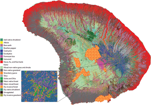
Figure 2. Species-specific land cover map for the island of Lāna‘i, based on expert-adjusted class posterior probabilities. Masked areas under the triangular polygons were infrastructure areas excluded from the analysis (Lāna‘i City, airport and other infrastructure). Example zoomed in areas are provided in appendices 10 and 11.

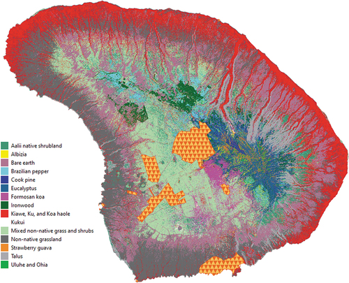
Figure 3. Example of individual class cover percent probability for the uluhe and ohia cover class.

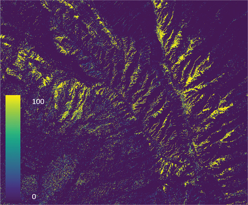
Table 3. Species-specific land cover area by class for the island of Lāna‘i, based on land cover classification including expert-adjusted class posterior probabilities.

	Area (km^2)	Percent land area
Aalii native shrubland	24.6	7.04
Albizia	1.4	0.41
Bare earth	59.1	16.91
Brazilian pepper	7.5	2.13
Cook pine	3.6	1.03
Eucalyptus	13.5	3.88
Formosan koa	6.4	1.83
Ironwood	9.3	2.67
Kiawe, Ku, and Koa haole	61.8	17.68
Kukui	0.7	0.21
Mixed non-native grass and shrubs	54.4	15.56
Non-native grassland	73.1	20.92
Strawberry guava	2.2	0.63
Talus	27.2	7.78
Uluhe and ohia	4.6	1.33

3.3. Mixed hierarchical land cover classification

Aggregating our species-specific class membership probabilities by community-specific classes also allowed us to generate maps of coarser non-species-specific vegetation classes (Figure 4), showing that dry invasive grasslands were the most widely distributed class, and mesic native forest was the least (Appendix 8). In total, dry invasive grassland, dry invasive forest, and unvegetated make up > 85% of the island’s area. Using our 66% certainty threshold, we created a mixed map between species-specific and community-specific categories in which, if the level of confidence in a given species-specific class was not met, the cover value was replaced with the projected coarser community-specific class (Figure 5). Although this mixed map includes classes from both classification levels, making it more typologically complex, it more reasonably reflects differences in model certainty across the landscape, displaying coarser class membership when finer species-specific projections yielded low certainty of class membership. In practical terms, because of our relatively low certainty threshold, only about 13% of the landscape reverted into coarser community-specific classes due to low species-specific class certainty (Appendix 9).

Figure 4. Community-specific land cover map for the island of Lāna‘i, based on land cover classification including expert-adjusted class posterior probabilities. Masked areas under the triangular polygons were infrastructure areas excluded from the analysis (Lāna‘i City, airport and other infrastructure).

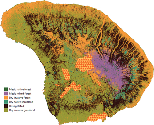
Figure 5. Mixed hierarchical land cover map for the island of Lāna‘i, based on land cover classification including expert-adjusted class posterior probabilities. Masked areas under the triangular polygons were infrastructure areas excluded from the analysis (Lāna‘i City, airport and other infrastructure). Map inset shows a high-elevation area with a mixture of species- and community-specific classes.

4. Discussion and conclusions

In this paper, we present a land cover modelling approach using machine learning to accurately classify vegetation into fine species-specific classes across the island of Lāna‘i, Hawaii. Our approach combines high-resolution satellite imagery with lidar-based geometric correction to overcome the limitations of previous efforts. Our results are a noticeable improvement over previously available land cover maps for the island (Appendix 10), showing very high accuracy for most vegetation classes, with overall accuracy generally above 95% based on polygon ground control data. We demonstrate that our approach can produce wall-to-wall species-level vegetation maps that can support conservation planning and monitoring on Lāna‘i and, if properly applied, in other topographically complex islands and regions.

Our attempt to improve our high-resolution land cover classifications with prior-based adjustments to class posterior probabilities had mixed but promising results. At a more basic level, visual inspection of results showed clear improvements between the original and prior-adjusted classifications (Appendix 11). The data-driven adjustment of posteriors led to more homogeneous, less noisy classifications. This is in line with similar past work that filtered posterior probability maps to improve classifications and that found that fine scale noise was significantly reduced (Guerrero-Curieses, Alaiz-Rodríguez, and Cid-Sueiro 2009). However, the data-driven posterior adjustment also led to more skewed representation of certain classes. In retrospect, this was likely given our data-driven prior was based on the training data, which was not systematically sampled across the landscape, thus leading to a potential skewed representation of class prevalence across the environmental predictors considered. On the other hand, the expert-driven priors, while not altering the overall classification accuracy, led to clearly improved classifications as visually inspected by experts. This indicates that the simple expert-led approach offers experts a way to further refine classifications based on local knowledge that typically is not possible on standard unsupervised classifications. However, the lack of improvement in accuracy does point to the need for a more representative ground control data in those areas where improvements were most visible. Expert-based classification refinement steps have been used elsewhere and shown to produce higher accuracies (Amarsaikhan et al. 2010).

Despite the high accuracy and detail of our vegetation classification approach and results, we still encountered limitations common to remote-sensing vegetation classification studies that may affect the applicability and generalizability of our own results. For instance, one main limitation of our analysis was the classifier’s confusion across similar land cover classes, such as different types of grasslands or shrublands, which may reduce the precision of our models. Another limitation is the problem of mixed pixels, which may contain more than one vegetation type within a single pixel. This problem may worsen as the number of considered land cover classes increases, leading to lower accuracy. We attempted to minimize these limitations by using a hierarchical classification approach, in which each 2 m pixel is assigned the most detailed class given a selected uncertainty threshold (i.e., the classifier may be unsure whether a given pixel is part of the eucalyptus or strawberry guava land cover but may be quite certain that it is part of a mesic mixed forest cover). However, this approach may not be sufficient to overcome some other limitations encountered. For example, some cover classes that are too small to be included in our models but still very important for conservation management (e.g., native dry forests) were omitted from our analysis. Moreover, the application of our method in areas where a greater diversity of native and introduced species exist may be increasingly challenging as the number of classes considered increase. One other limitation that was more challenging to overcome was that there were a few classes of interest to managers that did not have enough widespread distribution to provide enough data to train models to recognize them. These included primarily remnant native forest habitat that includes lama (Diospyros sandwicensis) and olopua (Notelaea sandwicensis) dry forests), but also included invasive plants (e.g., black bamboo (Phyllostachys nigra), mānuka (Leptospermum scoparium), faya (Myrica faya), cinnamon (Cinnamomum spp.), and common guava (Psidium guajava)). The same challenge of insufficient training samples will likely affect efforts to map recently established invasives, thus curtailing the use of our approach on efforts towards early eradication of invasive species on other islands.

The accuracy rates derived from the independent point-based model evaluation were lower but to some extent expected. Because that accuracy assessment was done using random points versus the continuous cover polygons, areas of less cover homogeneity likely were included, which may represent a more relevant accuracy estimate for pixel level map interpretation and use. However, the point-based validation of the vegetation classification also faced some limitations, which likely results in an underestimate for our independent measure of accuracy. One such limitation is the presence of mixels, or mixed pixels, which occur at the edge of different cover classes and may introduce uncertainty in class assignment for some of the assessed points (Crapper 1980). Additionally, despite our improved georectification, slight georectification errors particularly in very steep areas may have still led to misalignments between the satellite imagery and the actual ground features, and consequently on expert accuracy assessments (Shaker, Shi, and Barakat 2005). Furthermore, the uncertainty of the real cover class was inherently present in the point-based validation process, given that the assessment was conducted using aerial imagery. This reliance on aerial imagery may have limited the ability of experts to accurately distinguish between similar vegetation types or discern subtle differences in vegetation patterns. These limitations should be considered when interpreting the results of the point-based validation and when assessing the overall performance of the classification model.

Despite the limitations described above, our vegetation classification approach could be a valuable tool for land management and conservation purposes on Lāna‘i and other islands. One of the main applications of our vegetation maps may be to track the effects of planned ungulate suppression across the landscape. Ungulates are known to cause substantial damage to native habitats (Leopold and Hess 2017). However, without baseline vegetation data, it is difficult to assess the vegetation responses after ungulate removal. Our high-resolution maps can provide such baseline data and enable quantification of changes in bare soil exposure over time. At the highest elevations of Lāna‘i, Hawaiian petrel (Pterodroma sandwichensis) habitat is at risk due to encroaching non-native plant invasion. Uluhe once dominated large portions of Lānaʻi Hale, but conversion to invasive-dominated plant communities has reduced both native plant and animal density and diversity. The native uluhe cover identified in our analysis can serve to identify priority conservation and restoration areas for Hawaiian petrel and other endangered species recovery efforts, with future planned change analyses helping to identify areas of rapid invasive encroachment and stable native areas best suited for bird conservation efforts. Another application of our vegetation maps could be to inform erosion and sediment control planning, which is crucial for protecting water quality and coral reef health. Our maps can help identify areas with high sediment yield potential and prioritize mitigation measures accordingly. Furthermore, our maps can also be used for carbon inventory, which is relevant for climate change mitigation and adaptation strategies. By estimating the carbon stocks and fluxes of different vegetation types, and updating these analyses with future time steps, the contribution of Lāna‘i’s ecosystems to greenhouse gas emissions or sequestration can be estimated. Finally, our vegetation models provide new tools for understanding how vegetation responds to invasion and climatic changes, as well as to on-the-ground management efforts. By producing wall-to-wall species-level vegetation maps at regular intervals, we can better monitor the trends and patterns of vegetation dynamics on Lāna‘i and other islands.

Acknowledgements

Funding for this research came from the National Fish and Wildlife Foundation’s Kuahiwi a Kai program (NFWF Grant #66909). We kindly thank Paul Berkowitz for his review of the manuscript. Any use of trade, firm, or product names is for descriptive purposes only and does not imply endorsement by the U.S. Government.

Disclosure statement

No potential conflict of interest was reported by the author(s). Jon Sprague, Rachel Sprague and Kari Bogner were staff at Pulama Lanai, the entity in charge of land management for a large portion of the island of Lāna‘i. However, this is not deemed an interest, but instead a valuable asset to the effort that allowed us to have direct access to much of the landscape across the island to train and evaluate our models.

Data availability statement

The associated data release for this manuscript and associated metadata is available publicly at Berio Fortini (2024).

Supplementary Material

Supplemental data for this article can be accessed online at https://doi.org/10.1080/01431161.2024.2321465.

Additional information

Funding

The work was supported by the National Fish and Wildlife Foundation [NFWF Grant #66909].

References

- Aigbokhan, O. J., O. J. Pelemo, O. M. Ogoliegbune, N. E. Essien, A. A. Ekundayo, and S. I. Adamu. 2022. “Comparing Machine Learning Algorithms in Land Use Land Cover Classification of Landsat 8 (OLI) Imagery.” Asian Research Journal of Mathematics 62–74. https://doi.org/10.9734/arjom/2022/v18i330367.
- Amarsaikhan, D., H. H. Blotevogel, J. L. Van Genderen, M. Ganzorig, R. Gantuya, and B. Nergui. 2010. “Fusing High-Resolution SAR and Optical Imagery for Improved Urban Land Cover Study and Classification.” International Journal of Image and Data Fusion 1 (1): 83–97. https://doi.org/10.1080/19479830903562041.
- Balzotti, C. S., G. P. Asner, E. D. Adkins, E. W. Parsons, and A. Magrach. 2020. “Spatial Drivers of Composition and Connectivity Across Endangered Tropical Dry Forests.” The Journal of Applied Ecology 57 (8): 1593–1604. https://doi.org/10.1111/1365-2664.13632.
- Bayes, T., and Prince. 1763. “LII. An Essay Towards Solving a Problem in the Doctrine of Chances. By the Late Rev. Mr. Bayes F. R. S. Communicated by Mr. Price, in a Letter to John Canton, A. M. F. R. S.” Philosophical Transactions of the Royal Society 53:370–418. https://doi.org/10.1098/rstl.1763.0053.
- Benediktsson, J. A., J. A. Palmason, and J. R. Sveinsson. 2005. “Classification of Hyperspectral Data from Urban Areas Based on Extended Morphological Profiles.” IEEE Transactions on Geoscience and Remote Sensing: A Publication of the IEEE Geoscience and Remote Sensing Society 43 (3): 480–491. https://doi.org/10.1109/TGRS.2004.842478.
- Berio Fortini, L. 2024. High-Resolution Land Cover Maps of Lāna‘i. Hawai‘i: 2020: U.S. Geological Survey data release. https://doi.org/10.5066/P94TS6W6.
- Besnard, A. G., A. Davranche, S. Maugenest, J. B. Bouzillé, A. Vian, and J. Secondi. 2015. “Vegetation Maps Based on Remote Sensing are Informative Predictors of Habitat Selection of Grassland Birds Across a Wetness Gradient.” Ecological Indicators 58:47–54. https://doi.org/10.1016/j.ecolind.2015.05.033.
- Bobbe, T., H. Lachowski, P. Maus, J. Greer, and C. Dull. 2001. “A primer on mapping vegetation using remote sensing.” International Journal of Wildland Fire 10 (4): 277–287. https://doi.org/10.1071/wf01029.
- Chen, Q. 2007. “Airborne Lidar Data Processing and Information Extraction.” Photogrammetric Engineering and Remote Sensing 73 (2): 109–112. https://doi.org/10.14358/PERS.73.2.175.
- Chen, J., X. Chen, X. Cui, and J. Chen. 2011. “Change Vector Analysis in Posterior Probability Space: A New Method for Land Cover Change Detection.” IEEE Geoscience & Remote Sensing Letters 8 (2): 317–321. https://doi.org/10.1109/LGRS.2010.2068537.
- Chen, Q., and W. Lee, 2020. Mapping Individual Coconut Palm (Cocos nucifera) Trees in Urban Honolulu Using Deep Learning and Very High Resolution Remote Sensing Imagery, in: Hawaii Conservation Conference: Ola Ka ʻĀina Momona: Managing for Abundance. Presented at the Hawaii Conservation Conference: Ola Ka ʻĀina Momona: Managing for Abundance, Honolulu, HI.
- Civco, D. L. 1993. “Artificial Neural Networks for Land-Cover Classification and Mapping.” International Journal of Geographical Information Systems 7 (2): 173–186. https://doi.org/10.1080/02693799308901949.
- Crapper, P. F. 1980. “Errors Incurred in Estimating an Area of Uniform Land Cover Using Landsat.” Photogrammetric Engineering and Remote Sensing 46 (10): 1295–1301.
- da Silva, V. S., G. Salami, M. I. O. da Silva, E. A. Silva, J. J. Monteiro Junior, and E. Alba. 2020. “Methodological Evaluation of Vegetation Indexes in Land Use and Land Cover (LULC) Classification.” Geology, Ecology & Landscapes 4 (2): 159–169. https://doi.org/10.1080/24749508.2019.1608409.
- De Bruin, S., and B. G. H. Gorte. 2000. “Probabilistic Image Classification Using Geological Map Units Applied to Land-Cover Change Detection.” International Journal of Remote Sensing 21 (12): 2389–2402. https://doi.org/10.1080/01431160050030529.
- De Keersmaecker, D., R. Van De Kerchove, W. Zanaga, N. Souverijns, C. Brockmann, R. Quast, J. Wevers, et al. 2021. “Quantitative 3D real-space analysis of Laves phase supraparticles.” Nature Communications 12 (1): https://doi.org/10.5281/zenodo.5571936.
- Dias, E., R. B. Elias, and V. Nunes. 2004. “Vegetation Mapping and Nature Conservation: A Case Study in Terceira Island (Azores).” Biodiversity and Conservation 13 (8): 1519–1539. https://doi.org/10.1023/B:BIOC.0000021326.50170.66.
- Dinerstein, E., D. Olson, A. Joshi, C. Vynne, N. D. Burgess, E. Wikramanayake, N. Hahn, et al. 2017. “An Ecoregion-Based Approach to Protecting Half the Terrestrial Realm.” BioScience 67 (6): 534–545. https://doi.org/10.1093/biosci/bix014.
- Fassnacht, F. E., H. Latifi, K. Stereńczak, A. Modzelewska, M. Lefsky, L. T. Waser, C. Straub, and A. Ghosh. 2016. “Review of Studies on Tree Species Classification from Remotely Sensed Data.” Remote Sensing of Environment 186:64–87. https://doi.org/10.1016/j.rse.2016.08.013.
- Feret, J.-B., and G. P. Asner. 2013. “Tree Species Discrimination in Tropical Forests Using Airborne Imaging Spectroscopy.” IEEE Transactions on Geoscience and Remote Sensing: A Publication of the IEEE Geoscience and Remote Sensing Society 51 (1): 73–84. https://doi.org/10.1109/TGRS.2012.2199323.
- Ferreira, M. P., F. H. Wagner, L. E. O. C. Aragão, Y. E. Shimabukuro, and C. R. de Souza Filho. 2019. “Tree Species Classification in Tropical Forests Using Visible to Shortwave Infrared WorldView-3 Images and Texture Analysis.” ISPRS Journal of Photogrammetry and Remote Sensing 149:119–131. https://doi.org/10.1016/j.isprsjprs.2019.01.019.
- Guerrero-Curieses, A., R. Alaiz-Rodríguez, and J. Cid-Sueiro. 2009. “Cost-Sensitive and Modular Land-Cover Classification Based on Posterior Probability Estimates.” International Journal of Remote Sensing 30 (22): 5877–5899. https://doi.org/10.1080/01431160902787695.
- Guyon, I., J. Weston, S. Barnhill, and V. Vapnik. 2002. “Gene Selection for Cancer Classification Using Support Vector Machines.” Machine Learning 46 (1/3): 389–422. https://doi.org/10.1023/A:1012487302797.
- Haralick, R. M. 1979. “Statistical and Structural Approaches to Texture.” Proceedings of the IEEE 67 (5): 786–804. https://doi.org/10.1109/PROC.1979.11328.
- Haralick, R. M., K. Shanmugam, and I. Dinstein. 1973. “Textural Features for Image Classification.” IEEE Transactions on Systems, Man, and Cybernetics SMC-3 (6): 610–621. https://doi.org/10.1109/TSMC.1973.4309314.
- Jacobi, J. D., J. P. Price, L. B. Fortini, S. M. Gon III, and P. Berkowitz. 2017. “Baseline Land Cover.” In Baseline and Projected Future Carbon Storage and Carbon Fluxes in Ecosystems of Hawai‘i, edited by P. C. Selmants, C. P. Giardina, J. D. Jacobi, and Z. Zhu, 9–20. Reston, VA: U.S. Geological Survey Professional Paper 1834. https://doi.org/10.3133/pp1834.
- Jiang, D., Y. Huang, D. Zhuang, Y. Zhu, X. Xu, H. Ren, and J. A. Añel. 2012. “A Simple Semi-Automatic Approach for Land Cover Classification from Multispectral Remote Sensing Imagery.” Public Library of Science One 7 (9): e45889. https://doi.org/10.1371/journal.pone.0045889.
- Jung, M., P. R. Dahal, S. H. M. Butchart, P. F. Donald, X. De Lamo, M. Lesiv, V. Kapos, C. Rondinini, and P. Visconti. 2020. “A Global Map of Terrestrial Habitat Types.” Scientific Data 7 (1): 256. https://doi.org/10.1038/s41597-020-00599-8.
- Koerner, L. M., M. A. Chadwick, and E. J. Tebbs. 2022. “Mapping Invasive Strawberry Guava (Psidium cattleianum) in Tropical Forests of Mauritius with Sentinel-2 and Machine Learning.” International Journal of Remote Sensing 43 (3): 841–872. https://doi.org/10.1080/01431161.2021.2020364.
- Kursa, M. B., and W. R. Rudnicki. 2010. “Feature Selection with the Boruta Package.” Journal of Statistical Software 36 (11): 1–13. https://doi.org/10.18637/jss.v036.i11.
- Leopold, C. R., and S. C. Hess. 2017. “Conversion of Native Terrestrial Ecosystems in Hawai‘i to Novel Grazing Systems: A Review.” Biological Invasions 19 (1): 161–177. https://doi.org/10.1007/s10530-016-1270-7.
- Le Treut, H., R. Somerville, U. Cubasch, Y. Ding, C. Mauritzen, A. Mokssit, T. Peterson, and M. Prather. 2007. “Historical Overview of Climate Change.” In Climate Change 2007: The Physical Science Basis. Contribution of Working Group I to the Fourth Assessment Report of the Intergovernmental Panel on Climate Change, edited by S. Solomon, D. Qin, M. Manning, Z. Chen, M. Marquis, K. B. Averyt, M. Tignor, and H. L. Miller, 93–128. Cambridge UK: Cambridge University Press.
- Maxwell, A. E., T. A. Warner, and F. Fang. 2018. “Implementation of Machine-Learning Classification in Remote Sensing: An Applied Review.” International Journal of Remote Sensing 39 (9): 2784–2817. https://doi.org/10.1080/01431161.2018.1433343.
- McDonald, A. J., F. M. Gemmell, and P. E. Lewis. 1998. “Investigation of the Utility of Spectral Vegetation Indices for Determining Information on Coniferous Forests.” Remote Sensing of Environment 66 (3): 250–272. https://doi.org/10.1016/S0034-4257(98)00057-1.
- McKerrow, A. J., A. Davidson, T. S. Earnhardt, and A. L. Benson. 2014. “Integrating Recent Land Cover Mapping Efforts to Update the National Gap Analysis Program’s Species Habitat Map.” International Archives of the Photogrammetry, Remote Sensing and Spatial Information Sciences XL–1:245–252. https://doi.org/10.5194/isprsarchives-XL-1-245-2014.
- Olson, D. M., E. Dinerstein, E. D. Wikramanayake, N. D. Burgess, G. V. N. Powell, E. C. Underwood, J. A. D’amico, et al. 2001. “Terrestrial Ecoregions of the World: A New Map of Life on Earth: A New Global Map of Terrestrial Ecoregions Provides an Innovative Tool for Conserving Biodiversity.” BioScience 51 (11): 933–938. https://doi.org/10.1641/0006-3568(2001)051[0933:TEOTWA]2.0.CO;2.
- Oon, A., H. Z. Mohd Shafri, A. M. Lechner, and B. Azhar. 2019. “Discriminating Between Large-Scale Oil Palm Plantations and Smallholdings on Tropical Peatlands Using Vegetation Indices and Supervised Classification of LANDSAT-8.” International Journal of Remote Sensing 40 (19): 7312–7328. https://doi.org/10.1080/01431161.2019.1579944.
- Pesaresi, M., and J. A. Benediktsson. 2001. “A New Approach for the Morphological Segmentation of High-Resolution Satellite Imagery.” IEEE Transactions on Geoscience and Remote Sensing: A Publication of the IEEE Geoscience and Remote Sensing Society 39 (2): 309–320. https://doi.org/10.1109/36.905239.
- Richard, M. D., and R. P. Lippmann. 1991. “Neural Network Classifiers Estimate Bayesian A Posteriori Probabilities.” Neural Computation 3 (4): 461–483. https://doi.org/10.1162/neco.1991.3.4.461.
- Rollins, M. G. 2009. “LANDFIRE: A Nationally Consistent Vegetation, Wildland Fire, and Fuel Assessment.” International Journal of Wildland Fire 18 (3): 235. https://doi.org/10.1071/WF08088.
- Ruck, D. W., S. K. Rogers, M. Kabrisky, M. E. Oxley, and B. W. Suter. 1990. “The Multilayer Perceptron as an Approximation to a Bayes Optimal Discriminant Function.” IEEE Transactions on Neural Networks / a Publication of the IEEE Neural Networks Council 1 (4): 296–298. https://doi.org/10.1109/72.80266.
- Sales, M. H. R., S. de Bruin, C. Souza, and M. Herold. 2022. “Land Use and Land Cover Area Estimates from Class Membership Probability of a Random Forest Classification.” IEEE Transactions on Geoscience and Remote Sensing: A Publication of the IEEE Geoscience and Remote Sensing Society 60:1–11. https://doi.org/10.1109/TGRS.2021.3080083.
- Shaker, A., W. Shi, and H. Barakat. 2005. “Assessment of the Rectification Accuracy of IKONOS Imagery Based on Two‐Dimensional Models.” International Journal of Remote Sensing 26 (4): 719–731. https://doi.org/10.1080/01431160512331316847.
- Shivakumar, B. R., and S. V. Rajashekararadhya, 2018. Investigation on Land Cover Mapping Capability of Maximum Likelihood Classifier: A Case Study on North Canara, India. Procedia Comput. Sci., 8th International Conference on Advances in Computing & Communications (ICACC-2018) 143, 579–586. https://doi.org/10.1016/j.procs.2018.10.434
- Soille, P., and M. Pesaresi. 2002. “Advances in Mathematical Morphology Applied to Geoscience and Remote Sensing.” IEEE Transactions on Geoscience and Remote Sensing: A Publication of the IEEE Geoscience and Remote Sensing Society 40 (9): 2042–2055. https://doi.org/10.1109/TGRS.2002.804618.
- Ton, J., J. Sticklen, and A. K. Jain. 1991. “Knowledge-Based Segmentation of Landsat Images.” IEEE Transactions on Geoscience and Remote Sensing: A Publication of the IEEE Geoscience and Remote Sensing Society 29 (2): 222–232. https://doi.org/10.1109/36.73663.
- U.S. Geological Survey. 2017. 1/3rd Arc-Second Digital Elevation Models (DEMs) - USGS National Map 3DEP Downloadable Data. Collection: U.S. Geological Survey.
- Vaglio Laurin, G., N. Puletti, W. Hawthorne, V. Liesenberg, P. Corona, D. Papale, Q. Chen, and R. Valentini. 2016. “Discrimination of Tropical Forest Types, Dominant Species, and Mapping of Functional Guilds by Hyperspectral and Simulated Multispectral Sentinel-2 Data.” Remote Sensing of Environment 176:163–176. https://doi.org/10.1016/j.rse.2016.01.017.
- Valavi, R., J. Elith, J. J. Lahoz-Monfort, G. Guillera-Arroita, and D. Warton. 2019. “blockCv: An R Package for Generating Spatially or Environmentally Separated Folds for K-Fold Cross-Validation of Species Distribution Models.” Methods in Ecology and Evolution 10 (2): 225–232. https://doi.org/10.1111/2041-210X.13107.
- Wang, H., C. Liu, F. Zang, J. Yang, N. Li, Z. Rong, and C. Zhao. 2020. “Impacts of Topography on the Land Cover Classification in the Qilian Mountains, Northwest China.” Canadian Journal of Remote Sensing 46 (3): 344–359. https://doi.org/10.1080/07038992.2020.1801401.
- Wenger, S. J., and J. D. Olden. 2012. “Assessing Transferability of Ecological Models: An Underappreciated Aspect of Statistical Validation.” Methods in Ecology and Evolution 3 (2): 260–267. https://doi.org/10.1111/j.2041-210X.2011.00170.x.
- Zeferino, L. B., L. F. T. de Souza, C. H. D. Amaral, E. I. Fernandes Filho, and T. S. de Oliveira. 2020. “Does Environmental Data Increase the Accuracy of Land Use and Land Cover Classification?” International Journal of Applied Earth Observation and Geoinformation 91:102128. https://doi.org/10.1016/j.jag.2020.102128.
- Zhang, W., W. Li, and C. Zhang. 2016. “Land Cover Post-Classifications by Markov Chain Geostatistical Cosimulation Based on Pre-Classifications by Different Conventional Classifiers.” International Journal of Remote Sensing 37 (4): 926–949. https://doi.org/10.1080/01431161.2016.1143136.