HyperScout-1 inflight calibration and product validation

ABSTRACT

Earth observation aims at monitoring the Earth in increasingly more detail by improving the spatial, spectral and temporal resolution of image acquisitions. This can now be achieved in more cost-efficient ways by the miniaturization of instruments and platforms. New initiatives have emerged to accommodate hyperspectral instruments on CubeSats despite inherent platform limitations in terms of volume, power consumption, computing and downlink capacity. However, the adoption of CubeSat data for operational and scientific applications requires sufficient trust in dependability and data quality. Achieving reliable data quality from CubeSats remains challenging and requires advanced geometric, radiometric, and spectral calibration techniques. We present the successful in-orbit calibration of the HyperScout-1 mission. This In-Orbit Demonstration (IOD) mission, equipped with a miniaturized hyperspectral instrument based on Linear Variable Filter technology (LVF), was launched in 2018 by the European Space Agency (ESA). Rigorous inflight calibration has been applied to HyperScout-1 to ensure the accuracy of its data. The radiometric calibration of the HyperScout-1 instrument was performed vicariously based on modelled spectral radiances over a desert site. Independent validation using data from a CEOS RadCalNet site showed good radiometric accuracy with absolute radiometric errors <5%. Geometric errors due to inaccuracies in attitude measurements and sensor focal plane distortions were corrected using a bundle adjustment technique combined with matching to accurate Ground Control Points. This resulted in excellent geometric performance, with sub-pixel average absolute geolocation errors (~0.48 pixels across track and 0.51 pixels along track). The very limited data budget was a major challenge, forcing us to make some trade-offs in the calibration. Despite this, our robust vicarious calibration strategy allowed effective instrument calibration. As a result, the HyperScout-1 demonstrated the capability of an LVF Hyperspectral instrument on a CubeSat to deliver high-quality imagery and serve applications like land cover classification, change detection and disaster monitoring.

KEYWORDS:

• HypersScout-1
• CubeSat
• hyperspectral, linear variable filter
• radiometric
• geometric
• inflight calibration
• spectral calibration

1. Introduction

Earth observation aims at monitoring the Earth in increasingly more detailed ways by improving the spatial, spectral, and temporal resolution of image acquisitions. It is becoming increasingly possible to do so in a cost-efficient way by the miniaturization of instruments and platforms.

Large-scale monitoring is mainly performed using satellite platforms. Technological progress has enabled the development of smaller and more performant instruments and spaceborne platforms. However, the quest for compact, lightweight solutions continues, with nanosatellites and CubeSats being explored for Earth observation. Their lower cost allows for multiple platforms, improving spatial and temporal coverage.

Increasing the spectral resolution towards hyperspectral imaging opens enormous opportunities to solve more difficult Earth observation tasks. The additional spectral detail allows e.g. the discrimination between subtly different land cover classes to make a more accurate estimation of biophysical parameters, stress detection, pollution, water resources and quality etc. (Shen-En 2020).

However, hyperspectral imaging requires a radical shift in how to split light into separate wavelengths. Conventional multiband imagers often use absorption filters, with a specific filter mounted on an image detector for each band. As it is not practical to scale this technology to, hyperspectral instruments use different physical principles to separate light into different wavelengths.

Traditional instruments such as APEX (Itten et al. 2008), ENMAP (Guanter et al. 2015) and PRISMA (Cogliati et al. 2021) use prisms to disperse light per wavelength onto a frame detector. They acquire scenes line by line like conventional pushbroom-line scanners and achieve highly accurate results because all light is used. Similar to laboratory imaging spectrometers, they tend to be large, heavy, complex and costly in development and operation (Hueni et al. 2009).

To create more compact instruments, alternative technologies are increasingly being used. Replacing prisms by gratings which can be integrated on a mirror of the optical system reduces complexity and size.

Mounting thin-film interference filters on image detectors offer a simpler, compact instrument design. A Fabry–Pérot interferometer is an optical cavity consisting of two parallel reflecting surfaces (Macleod 2003). Because of interference, only light of a narrow spectral band passes through, and the wavelength of the band is governed by the thickness of the cavity. A cavity with varying thickness creates a ‘Linear Variable Filter’ (LVF), which offers a gradual variation in the spectral response. The filters block most light, resulting in a somewhat lower performance compared to other hyperspectral instruments (Moreau et al. 2012). This is however compensated by the fact that, with suitable optics, the 2D imaging detector receives light from a complete 2D scene instead of dispersed light from a line of that scene (the snapshot advantage, as advocated by (Hagen 2012)).

Because the imaging concept of an LVF-based system differs fundamentally from a traditional line scanning hyperspectral imager, the approach to reconstruct the hypercube from the images acquired needs to be revised.

After the first concept of a hyperspectral satellite based on LVF technology was proposed in (Maresi et al. 2010), multiple initiatives have evaluated the merits and limitations of LVF technology. In the European Space Agency (ESA) CHIB project (Moreau et al. 2012), a simulation study was performed to test this new technology. In the $\mathit{\mu }$TMA study, miniaturization of an LVF-based imager to fit a CubeSat was investigated (Zuccaro, Deep, and Grabarnik 2012) and the feasibility for producing a µ-TMA compatible with a CubeSat was demonstrated. It was concluded that the performance of such a system is lower than for traditional systems, but it can still allow to perform useful application work provided that signal-to-noise ratios are not too low. Significant improvements to the current technology have been investigated. The direct deposition of filter material on sensors eliminates alignment issues of the classical LVF filter and allows a more flexible filter design (Livens et al. 2014). It should be noted that the main focus of previous initiatives has been on the core of the hyperspectral instrument i.e. the hyperspectral focal plane.

Besides the hardware challenge of adapting hyperspectral technology to a CubeSat platform, data volume and processing issues also hinder the development and proliferation of hyperspectral CubeSat missions. Current satellite Earth observation systems can acquire vast amounts of data, but are limited by their downlink capacity, especially for hyperspectral data acquisition CubeSat systems’ limited power further reduces data downlink volumes, making operational downlinking of all raw image data captured on a hyperspectral CubeSat system unrealistic.

Recent initiatives aim to fit hyperspectral instruments on CubeSats and Nanosats, despite their size, power, computing, and downlink limitations. The HyperScout-1 In-orbit Demonstration (IOD) mission launched by the European Space Agency (ESA) in 2018 aimed to set new benchmarks and combine cutting-edge hyperspectral technology with revolutionary CubeSat capabilities (Marco Esposito and Marchi 2015; Esposito et al. 2018). The project was funded by a consortium led by Cosine Measurement Systems B.V (Netherlands) with funding from the ESA GSTP (General Supporting Technology Program), including VITO NV (Belgium), S[&]T AS (Norway) and TU-Delft (Netherlands). HyperScout-1 was developed to demonstrate that hyperspectral acquisition from nanosatellite platforms is indeed possible by exploiting recent advances in optics, filtering, detection, and advanced on-board computing technologies. HyperScout-1 onboard the GomX-4 6 U CubeSat was launched on 2 February 2018. It carries a hyperspectral payload based on the LVF technology and operates in the VNIR. Thanks to its large field of view (325 km at 540 km altitude) and its on-board intelligence, HyperScout-1 can enable a variety of land and vegetation applications where cost-effectiveness and timeliness are critical (Esposito et al. 2018).

In this paper, challenges related to images processing and the calibration of HyperScout-1 data are discussed. We first describe the HyperScout-1 Image product, followed by a detailed description of the inflight calibration approaches (geometry, radiometry and spectral). Finally, the inflight radiometric and geometric performances of HyperScout-1 were discussed.

2. HyperScout-1 Mission description

HyperScout-1 is a Hyperspectral In-orbit Demonstration mission launched in February 2018 on-board the GomX-4 6 U ESA CubeSat developed by GomSpace ApS (Denmark) (Leon and Koch 2018). The payload is the Cosine powered hyperspectral imaging solution for nano, micro and larger satellites (Esposito and Marchi 2019). It is based on the Linear Variable Filter technology, acquiring data in the Visible and Near-InfraRed (VNIR) spectral range. The satellite is flying at 540 km allowing a wide field of view (325 km) and 80 m ground sampling distance. HyperScout-1 was designed as a CubeSat payload, and because of its small size and high processing power, it can be used in a variety of applications ranging from vegetation monitoring to change detection and water applications.

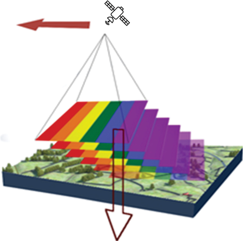
HyperScout-1 uses pushframe imaging technique that acquires image frames in a pushbroom manner (see Figure 1). Instead of using a 1D line sensor, a pushframe camera uses a 2D detector, which repeatedly captures 2D images, called frames. Because image frames are captured with overlapping footprints, the construction of a final image requires mosaicking the frames together. Re-projection of the frames based on the camera’s imaging geometry is therefore necessary.

Figure 1. HyperScout-1 pushframe imaging technique.

2.1. Instrument description

The main characteristics of the instrument are summarized in Table 1. The telescope is a Three Mirror Anastigmatic (TMA), which achieves diffraction limited optical performance over the whole field of view, for maximum imaging quality and spatial resolution. This is combined with a small F-number in a very small volume by using aspheric and freeform mirrors. Straylight is controlled by baffles at the entrance and between telescope elements.

Table 1. HyperScout-1 main characteristics.

Parameter	Value
Orbit	Sun Synchronous, 540 km altitude, LTDN 15:00 hrs
Field of view	31° (across track) × 16° (along track)
Focal length	41.25 mm
F-number	4
Ground Sampling Distance	80 m @ 540 km
Swath	325 km @ 540 km
Pixels	4096 (across) × 3072 (along)
Pixel size	5.5 µm
Spectral range	425-975 nm
Number of spectral bands	50
Spectral resolution	15 nm (average)
Dynamic range	12 bit
Mass	1.3 kg
Nominal data throughput	45.5 MB/s

The imager is based on a CMV12000sensor from AMS (AMS 2022). A linear variable filter (LVF), deposited on a glass substrate, is mounted directly onto the sensor. The filter does not cover the entire sensor but an area with full width (4096 columns) and a smaller height (about 1850 lines), fitting the optical field of view.

As introduced in section 1, it is an interference filter which only transmits the light of a narrow spectral band optical performance over the whole field of view, to achieve the maximum imaging quality and spatial resolution. The linear thickness variation, aligned with the along track direction of the sensors, results in a continuous variation in the transmitted wavelength within the range of 425 nm to 975 nm.

2.2. Spectral band and resolution

Because of this, every detector line is sensitive to a different wavelength and could be regarded as a separate spectral band. This would result in 1850 different bands. The FWHM of those bands varies between 16 nm and 26 nm (average: 21.5 nm), while the spectral sampling (difference between central wavelength of adjacent bands) is about 0.3 nm. This means that the spectrum is strongly oversampled, and the bands contain strongly correlated data. This is also clear in Figure 3, where we plot the spectral responses of a small subset of bands. The spectral responses as given are the product of the transmission of the filter and the quantum efficiency (QE) of the sensor.

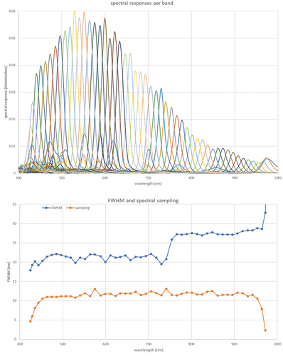
Note that the maximal sensitivity varies, caused by differences in the quantum efficiency of the sensor. The spectrum can be represented with a much smaller set. Therefore, over the whole sensor, sets of 36 adjacent lines are grouped and regarded as a single spectral band. The number of lines per group was chosen so that for every spectral band, a gapless acquisition is achieved, considering the available frame rate. The grouping results in a total of 51 bands, of which 6 bands with bad or very low spectral response are omitted, resulting in 45 usable spectral bands.

The pooling of 36 lines results in a combined band with a spectral response which is the average of its constituents, as plotted in Figure 2 (blue line with blue circles). Its FWHM is larger than the FWHM of the individual lines. The FWHM and spectral sampling of full set of 45 combined bands are plotted in Figure 3. The average FWHM is 21.5 nm, and average sampling is 11 nm, so the whole spectrum is sampled sufficiently. A less dense sampling could be used to reduce data volume, still covering the full spectrum but with reduced spectral detail.

Figure 2. HyperScout-1: example spectral responses of a set of 36 adjacent lines. Blue line with circles shows the combined spectral response of a single spectral band.

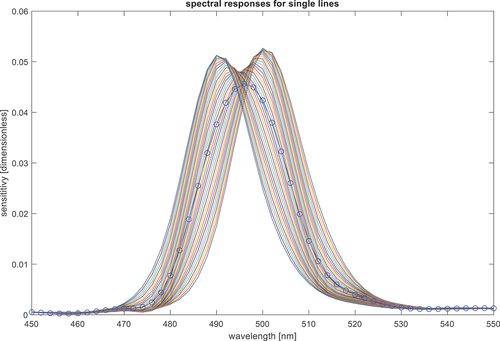
Figure 3. HyperScout-1 instrument spectral band characteristics (top) spectral responses (bottom) full width half max (blue line) and spectral sampling (orange line).

2.3. Focal plane layout

The focal plane layout is composed of multiple frames defined in a nested fashion, whereby the origin of the child frame is defined relative to the origin of the parent frame (Figure 4). The origin of a frame is defined as the top left corner (0,0). Inheritance of nested frames (parent → child) is as follows:

Figure 4. Focal plane layout (a) is the showing the different frame arrangement (sensor, frame, optical and illuminated). (b) is showing the sensor and LVF configuration geometry. The north vector is counter to the satellite motion vector for acquisitions on the descending node, which is the nominal case for out of eclipse acquisitions. The pixel size of the CMV12000 is 5.5 µm whereas the focal plane is 41.25 mm (source: Cosine measurement systems).

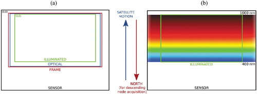
SENSOR → FRAME → OPTICAL →ILLUMINATED.

Their definitions are as follows:

• SENSOR : the full size of the CMV12000 (AMS 2022).

• FRAME: the area of the SENSOR read out by the Front-end electronics (includes electrical black pixels)

• OPTICAL: the optically active pixel area (includes optical black pixels)

• ILLUMINATED: the region of the sensor illuminated by the telescope

2.4. Onboard data processing

HyperScout-1 can acquire vast amounts of data; therefore, the bottleneck of the technology is often the limitation in downlink capacity. A workable solution is found by performing on-board processing which maximally reduces the data volume to a manageable level. The challenge is to be able to do the processing which is traditionally executed on large data centres within the limited resource of on-board computers and in the absence of the metadata which is typically used in on-ground processing approaches.

HyperScout-1 is equipped with an on-board data handling system (OBDH) capable of processing captured data in real-time and generating Level2 products. The goal is to enable early warnings by downloading processed geophysical data products with coordinate information, rather than raw data (Soukup et al. 2016).

3. Product overview

HyperScout-1 products comprise the following levels of processing (see Table 2):

Table 2. HyperScout-1 products description.

Processing level	Description	Processing unit
Level-0	Files containing: instrument data at full resolution (Digital Number DN frame image) annotated with instrument housekeeping data and a timestamp. platform ancillary data satellite position, velocity satellite attitude information timestamp all meta data needed for the following processing step towards Level 1a shall be included.	Frame image (see explanation below)
Level-1A	Level-0 plus associated geo-location information including: latitude/longitude grid for each pixel of the frame image solar angles (zenith and azimuth) grid for each pixel of the frame image (if required) satellite viewing angles (solar and azimuth) grid for each pixel of the frame image (if required).	Frame image
Level-1B	Level-1A radiometrically corrected unprojected top of atmosphere (TOA) radiance at pixel level Radiometric quality status map at pixel level	Frame image
Level-1C	Level-1B containing all unprojected reshaped spectral bands	Band image (see explanation below)
Level-2A	Level-1C mapped and projected into a uniform space grid (projected TOA radiance). Each spectral band is projected and the spectral cube is then reconstructed.	Band image

Note that the processing steps are defined for two types of unit processing:

1. The frame image is defined as a single image acquired in one snapshot at time t by the 2D detector spectral array. The across track direction represents the spatial information of a single spectral band while the along track represents the spectral axis. The processing from the Level 0 up to the Level 1b is performed on a frame image basis.

2. The band image is defined as an image associated with a single spectral band reconstructed from multiple frame images acquired at various times by the 2D detector array. The across track and the along track directions contain the spatial information of one single spectral band. The process to convert the frame image into a band image is explained in the next paragraph. Note that the band image at level-1C is still unprojected data and thus cannot be used as such to reconstruct the spectra. Therefore, processing from the level-1C up to the Level-2A is required and performed on a band image basis.

3.1. Level-1 processing

3.1.1. Geometric processing (level-0 to level-1A)

For each position of the HyperScout-1 satellite, a geolocation step was performed to determine the geographical coordinates (latitude, longitude, and height) of the earth sample seen by a pixel of the satellite sensor. This process calculates the intersection of the satellite line of sight with an Earth model and corrects for digital elevation effects. The satellite position and velocity were interpolated for each frame image using an orbital propagator model or a simple Lagrangian interpolation polynomial. The frame image timestamp information was retrieved from the level-0 data. The transformation matrices between different reference frames (platform, payload, instrument, and detector) were calculated using the level-0 satellite attitudes information together with the polar motion data, earth rotation, precession, and nutation data. To refine the geolocation accuracy, the geometric processing model initially uses the geometric pre-flight Instrument Calibration Parameters file (ICP) measured in the laboratory. This ICP file is regularly updated by the inflight geometric calibration suite if needed. The ICP file contains the line of sight of each pixel in the frame image.

In addition, the geometric processing model calculates the necessary solar and satellite viewing angles (zenith and azimuth), required for further radiometric and atmospheric processing. The output of the geometric processing is level-1A data for each acquired frame image.

3.1.2. Radiometric processing (level-1A to level-1B)

This section describes the radiometric processing applied to the HyperScout-1 raw data to derive Top of Atmosphere (TOA) radiance values. The following radiometric model is used. The Digital Number DN^k is first corrected for dark current (DC), which accumulates with integration time but is independent of incoming light, and Fixed Pattern Noise (FPN), which is a fixed offset signal. Next, it is converted to at-sensor radiance (L^k) using the absolute conversion factor $A^{\mathit{k},\mathit{T}}$. The index k can refer to a spectral line or a spectral band in which lines are pooled together.

This factor comprises three effects:

• Overall absolute calibration coefficient (link between DN and radiance)

• Pixel response non-uniformity (PRNU)

• Relative Response Function (inter band)

The total conversion, including the integration time (IT) can be written as:

$L^k=\frac{D{N}^k-\left(\mathit{D}{C}^{\mathit{k},\mathit{T}}\times \mathit{IT}+\mathit{FP}{N}^k\right)}{A^{\mathit{k},\mathit{T}}\times \mathit{IT}}$

The coefficients $A^{\mathit{k},\mathit{T}}$, $\mathit{D}{C}^{\mathit{k},\mathit{T}}$ and $\mathit{FP}{N}^k$ are found in the pre-flight radiometric Instrument Calibration Parameters. The output of the radiometric processing is level-1B for each frame image.

3.1.3. Data reshaping (level-1B to level-1C)

All processing up to the level-1B was performed on a frame image basis. The geo-positioning information and Top of Atmosphere radiance values related to a single spectral band are contained in all acquired frame images. The frame image format cannot be used for further processing and all data representing a single spectral need to be assembled into a band image format. Therefore, a data reshaping step was performed to convert the frame image to a band image. The output of this step is level-1C which contains data separated into spectral band images.

3.2. Level-2 processing

A level 2 image is the result of mapping (a number of spectral bands) of a level-1C image to a given user projection grid. Universal Transverse Mercator (UTM) projection was used for all HyperScout-1 products. In the projection procedure (Riazanoff 2004; Sterckx et al. 2014), an inverse model is first used to determine for a given (x, y) pixel in the level 2 data grid its corresponding pixel and line (p, l) coordinates in the level 1 data. This is performed using a polynomial predictor functions that relate the (x, y) coordinates to the (p, l) coordinates. Once the (p, l) coordinates are known, for each spectral band of the level 2 data, the pixel value to be mapped can be determined using a bicubic interpolation filter. Note that the projection step is applied separately to each unprojected spectral bands because each spectral band has its own ground spatial extent and coverage.

4. HyperScout-1 data

Table 3 and Table 4 summarize all the acquired HyperScout-1 scenes after the launch that are used for the payload commissioning phase. It describes the acquisition dates, acquired region of interest (ROI) together with targeted applications. Due to limited HyperScout-1 downlink capacity, it was not possible to download ROIs at the full frame size. Choices were made to significantly reduce the size of the acquired data while maintaining sufficient content for testing, calibration, and validation purposes. For instance, the ‘20181108.01_Algeria’ frames 1, 4, 7, 10 and 13, were acquired with full swath whereas the rest was acquired with half of the swath. Image cropping was also applied on-board for certain ROIs (Table 3), as an example, ‘20181107.02_Railroad_Valley’ area includes a full set of frames for a small spatial region, appropriately sliced such that the illuminated area of each frame represents the same area on ground allowing a complete acquisition of all spectral bands above this ROI. Despite the small spatial extent, the image content was sufficient for radiometric calibration purposes as the radiometric targeted ROI was very small and did not require full frame mode acquisition. The ROIs used in this study are highlighted in grey in Table 3.

Table 3. HyperScout-1 acquisition scenes and their targeted purposes (source: Cosine measurement systems).

Date	Region of interest	Number of frames	Acquired data	Applications	ROI	Comments	Used for calibration
01-Nov-2018	Ceylanpinar, Turkey	>61	Hyperspectral data cube	Crop requirements	Selected ROI	-	Used for science application + geometric calibration
07-Nov-2018	Libya4 desert	>61	Hyperspectral data cube	Spectral & radiometric response	Selected ROI	-	Used for radiometric calibration
07-Nov-2018	Railroad Valley, Nevada	>61	Hyperspectral data cube	Spectral & radiometric response	Selected ROI	-	Used for radiometric/geometric calibration
08-Nov-2018	Algeria2	15	Subsequent frames for co-registration	Geometric processing	Half frame	-	Used for geometric calibration
14-Nov-2018	Doukkala, Maroc	>61	Multispectral data cube	Crop requirements	Half frame	Partially clouded	Received but lacking telemetry data
20-Nov-2018	Bahamas	>61	a. Hyperspectral data cube b. Multispectral data cube	Bathymetry, Water monitoring	a. Selected ROI b. Half frame	Sparsely clouded	Used for science application + geometric calibration

Table 4. HyperScout-1 acquired ROIs and their instrument settings. ACT means across track and ALT means along track (source: Cosine measurement systems).

ROI name	Date; Time [UTC]	LAT; LON	Region of interest	ROI ACT pixel range; ROI ALT pixel range	Exposure time	Offset setting
20181107_Ceylanpinar	1 Nov 2018; 11:43:55	+37,016; +39,814	Ceylanpinar, Turkey	2080:3744; 24:1880	10 ms	1850
20181107.01_Libya4	7 Nov 2018; 12:46:17	+29,568; +23,655	Libya4 desert	1568:3232; 24:1856	7 ms	1850
20181107.02_Railroad_Valley	7 Nov 2018; 22:11:08	+39,380; −115,659	Railroad Valley, Nevada US	1248:3232; 24:1856	10 ms	1850
20181108.01_Algeria	8 Nov 2018; 14:58:00	+26,428; +4,672	Algeria2	416:3744; 24:1856	8.5 ms	1850
20181120_Bahamas	20 Nov 2018; 19:09:48	+22,569; −74,034	Bahamas	2080:3744; 24:1880	10 ms	1850

5. Level-1 inflight calibration strategy

5.1. Spectral calibration approach

Pre-flight calibration of hyperspectral instruments includes determining the precise characteristics of each spectral band. For HyperScout-1, measurements with a monochromator were conducted to determine the spectral sensitivities, from which the main per band parameters including central wavelength and spectral width were derived.

The performance of the instrument is however likely to change after launch and during the mission lifetime (Guanter, Richter, and Moreno 2006), often causing spectral shifts and/or distortion effects. Inflight spectral calibration is carried out to detect and correct such deviations. This is generally based on detecting sharp peaks in the measured spectrum and correlating them with expected peaks at well-known wavelengths.

For the HyperScout-1 mission, the data budget did not allow a comprehensive campaign for spectral calibration. However, in tandem with the radiometric calibration activities, an in-orbit verification based on the observation of atmospheric absorption bands was carried out, using a method similar to the one described in (Bo-Cai Gao, Yang, and Yang 2004).

The essence of the method is to compare the wavelength of atmospheric absorption bands over a known test site, obtained from an actual HyperScout-1 acquisition with the same absorption bands obtained independently. The independent spectrum is obtained from RadCalNet (CEOS https://www.radcalnet.org).

The procedure comprised following steps:

1. Convert acquisition to radiance spectrum.

2. Establish reference radiance spectrum.

3. For both, identify a few clear spectral features distributed over the spectral range.

4. Determine exact wavelength of the features in both spectra.

5. Compare wavelengths to estimate spectral shift.

This results in an estimate of spectral shift for three points in the spectrum, giving a reasonable indication of potential shifts over the entire spectrum. Results are reported in Section 6.1.

5.2. Radiometric calibration

The radiometric model describing the conversion from digital number to at-sensor radiances is presented in section 3.1.2. Its parameters are initially established during the pre-flight calibration. However, the radiometric performance may be impacted once in orbit due to outgassing phenomena during launch, ageing of the optical parts, and cosmic ray damage. To achieve and maintain radiometric performance, these parameters need to be monitored inflight and updated as needed. For missions with longer lifetimes, this is a repeated process. For HyperScout-1, the goal was to demonstrate successful radiometric inflight calibration establishing a single set of calibration parameters, which are then assumed to remain valid for all regular acquisitions made during the mission lifetime.

For small missions, a preferred way to establish accurate inflight calibration is making intercomparisons with other well-calibrated hyperspectral missions, using Simultaneous Nadir Overpass (SNO) observations. However, at the time when Hyperscout-1 was launched, important missions like EnMAP, EMIT or PRISMA were not yet available. Because the opportunities for such observations were extremely limited, we did not include them in the calibration plan, but opted to use vicarious calibration sites only. For current and future missions, a combination of both approaches is recommended.

The main limitation of the mission is its very limited data budget. This implies that only very few images could be acquired specifically for the purpose of inflight calibration, limiting the achievable accuracy and possibilities to perform verification.

5.2.1. Dark signal calibration

The pixels of a detector produce a nonzero signal in the absence of light. This is a combination of fixed pattern noise (FPN) and dark current (DC). FPN can vary strongly from pixel to pixel, but each value remains constant, so it can be corrected completely. The root causes of FPN are unavoidable process variations in the manufacturing of the detector at pixel level, including all its accompanying electronics. DC is proportional to the integration time, depends on temperature and may also be impacted by irradiation in space. Both FPN and DC can be determined in a pre-flight calibration campaign and corrected. For DC, a pre-flight characterization at different temperatures is necessary. Three temperatures were used (15°C, 25°C and 35°C). After this, the radiometric processing can correct for both effects. Unlike the FPN, DC is statistical in nature and thus after correcting for its average value per pixel, a small variance dark error remains.

In the initial calibration plan, an option was foreseen to perform inflight dark current calibration using dedicated acquisitions over dark oceanic sites. However, pre-flight results showed that FPN was dominant over DC. Changes in DC after launch would most likely not meaningfully influence the radiometric processing. Therefore, inflight DC calibration was omitted.

5.2.2. Absolute calibration

The goal of the inflight absolute calibration is to verify the (pre-flight) absolute conversion factor $A^{\mathit{k},\mathit{T}}$ (as described in section 3.1.2) and if needed, establish new values for it. This can be performed by acquiring images over sites which are well characterized. Then modelled spectral radiances ($L_{mo\mathrm{del}}^k)$of the sites can be compared to spectral radiances ($L_{pr\mathrm{eflight}}^k=A_{pr\mathrm{eflight}}^K\ast \mathit{D}{N}_{acq}^K)$obtained from the acquisitions ($\mathit{D}{N}_{acq}^K$) using pre-flight calibration parameters ($A_{pr\mathrm{eflight}}^K$). By doing so for every wavelength of the spectrum, a new set of inflight calibration coefficients ($A_{in\mathrm{flight}}^K$) can be obtained as follows:

$A_{in\mathrm{flight}}^K=\frac{L_{m\mathrm{odel}}^K}{L_{p\mathrm{reflight}}^K}{A}_{pr\mathrm{eflight}}^K$

We will use bright stable desert sites and thus carry out a ‘desert calibration’ method, as described in (Govaerts, Sterckx, and Adriaensen 2013). We will use both a standard reference site (Railroad Valley) for which radiometric values are available from RadCalNet (CEOS) and a desert site (20181107.01_Libya4) for which we performed our own modelling with the Optical Sensor Calibration with simulated Radiance (OSCAR) RPV model, originally developed for ESA’s PROBA-V mission (Govaerts, Sterckx, and Adriaensen 2013).

Establishing accurate absolute calibration requires a sufficient number of calibration acquisitions for which reference data is available. A well-designed calibration effort should contain at least these three steps: 1) Verification of the pre-flight calibration parameters, 2) Determination of new inflight calibration parameters and 3) Validation of the correctness of the new parameters.

Steps 2 and 3 only need to be performed if the verification in step 1 indicates the needs for updating the parameters. In step 3, it is essential to perform the validation on data which is independent from the data used in step 2. In step 1 however, it is acceptable to use the same data as step 2 or Step 3.

As can be seen from Table 3, only two suitable acquisitions were available (20181107.01_Libya4 and 20,181,10702_Railroad_Valley). This implies that only minimal calibration strategy can be performed, using one of the images for step 2, and the other for step 3. The image which is most likely to yield the most accurate results should be used in the calibration step (it is preferred to calibrate accurately and poorly verify than vice versa). For both acquisitions, an independent reference model is available to provide modelled radiances, suitable for establishing a correspondence to the acquired data.

The ‘20181107.01_Libya4’ site has the advantage that it is a large site, so more statistics could be collected. However, due to its lack of clear features, no exact geometric correspondence could be established for this area so a strict matching using the exact same area is not possible. The Railroad valley site is smaller, making it harder to collect enough statistics for all spectral bands. However, accurate geometric correspondence is available so the exact area can be used. This area is very uniform so less statistical averaging is necessary.

Since reflectances as provided by RadCalNet are widely used as reference for many missions, we were initially inclined to use this for calibration. However, in an earlier study (Sterckx and Wolters 2019), it was shown that BRDF effects significantly influence the results for the Railroad Valley site. A major difference was reported in reflectance values depending on the acquisition viewing angle. ‘20181107.01_Libya4’ site. Since the RadCalNet portal does not provide BRDF data/information, no correction for BRDF effects could be made. We also do not have acquisitions with different viewing angles over the same areas, so we cannot assess or correct such effects. Therefore, we preferred to perform calibration using the ‘20181107.01_Libya4’ image and the associated OSCAR RPV BRDF model (Govaerts, Sterckx, and Adriaensen 2013).

As described in Section 2.2, every line of the sensor has a different spectral response, but 36 adjacent lines are combined into a single band for the image products. Performing absolute calibration on the product bands leads to strong artefacts because the lines contributing to the same bands all have different responses, and thus need to be calibrated differently. Therefore, we adopted a line-based calibration methodology in which each line of the sensor is calibrated separately.

5.3. Geometric calibration

The limiting factor of using HyperScout-1 and, in general, CubeSat for EO purposes is their geometric instability (>0.1°). Environmental monitoring and land cover management applications (e.g. change detection) require a high geometric performance (subpixel accuracy). These applications usually analyse dynamic phenomena that result in changes to Earth surface. Changes in dynamics are solved using change detection techniques to automatically label changes occurring between images of the old state of a scene and images of its current state. Relative instability in the geolocation of on-ground pixels may drastically impact the performance of change detection techniques, limiting their capability to detect substantial and real changes. Improving the geolocation accuracy by developing robust on-ground image-based techniques is therefore a prerequisite for offering reliable and affordable products from the HyperScout-1 Instrument. New and innovative geometric calibration approaches have been envisaged to enhance the geolocation accuracy to an acceptable value. The aim of such techniques is to estimate and monitor exterior orientations (i.e. satellite positions and boresight misalignment angles) and interior orientation deformations.

HyperScout-1 camera’s geometric distortions are calibrated in detail before launch, but it cannot be guaranteed that the geometry does not change during launch. Perturbations and instabilities are caused by post-satellite launch, optical distortions, thermal-related distortions of the focal plane, or exterior orientation inaccuracies.

The inflight geometric calibration estimates the boresight misalignment angles and interior orientation parameter values included in the geometric Image Calibration Parameters (ICP) file. The quality of inter-band data co-registration and the absolute geolocation accuracy of the final HyperScout-1 image product depend on the quality of the geometric calibration data. In classical push-broom sensor-based satellite missions, the geometric calibration parameters are estimated using a large number of globally distributed Ground Control Points (GCP). The interior and exterior parameters are estimated via a weighted and constrained inversion model, which is based on an iterative least-squares adjustment. Geometric calibration algorithms relevant to linear push-broom scanners require serious modifications to correctly model the 2D frame sensor of the HyperScout-1 instrument.

However, because the HyperScout-1 instrument is not a classical push-broom scanner, other geometric inflight sensor calibration techniques have been explored, for example, techniques originally developed for frame UAV/airborne sensors. The choice of the final inflight calibration method depends strongly on the final platform stability/performance parameters. Because the platform performances are not sufficient to correctly process the HyperScout-1 image data using direct georeferencing, refinement of the exterior image orientation parameters was necessary.

5.3.1. GCPs database generation

A common approach for in-orbit absolute geometric calibration is based on the use of reference Ground Control Points and rigorous geometric sensor model. GCP selection for use in image geo-referencing is required to provide an external positional reference coordinate that allows the internal geometry of the image to be matched with the real terrain coordinates for the area imaged by the sensor. GCPs are selected for a well-delineated, high-contrast object with discrete geometry (e.g. a corner) that is recognizable in the image. An alternative to manual GCP selection is the use of template matching, which is based on locating a known reference image in the newly acquired sensor image (see section 5.3.3).

The Landsat Global Land Survey (GLS) 2010 dataset (http://glcf.umd.edu/data/gls/) was used to extract GCPs. GLS 2010 is a collection of precision orthorectified Landsat ETM+ scenes (from Landsat-7 and 8) with spatial pixel resolutions of 15 and 30 m for the panchromatic and visible bands, respectively. These datasets comprise all nine Landsat ETM+ spectral bands and are in a Universal Transverse Mercator (UTM) map projection. The geolocation accuracy of this product was prespecified to be below 25 m (RMSE) globally (Liu et al. 2022).

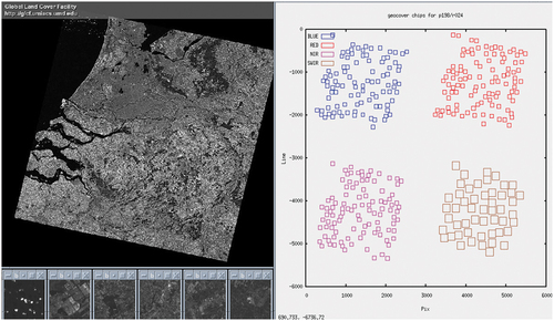
GCP chips (Figure 5) were extracted from bands 1, 3, 4, and 8 of the GLS 2010 scenes. The Moravec interest operator algorithm was applied to the images to determine the interest points using a specified window size suitable for satellite data. The global GCP chip database was constructed in advance and used in geometric calibration software.

Figure 5. Example of GCPs extracted from GLS2010; left: example of Landsat-7 tile, right: extracted GCPs in 4 spectral bands.

5.3.2. Coarse boresight refinement

After the HyperScout-1 launch, the absolute geo-pointing performance suffered from a large bias, where the line of sight was off by a few kilometres from the true ground target. The direct application of the traditional GCPs chip matching technique requires a large search area to find the geometric absolute shift by comparing a template image to the searching image. To reduce the search area and consequently the computation time for finding matches, we coarsely refined the boresight and estimated the large bias in the boresight angles to be removed to bring the absolute geolocation error to reasonable values (~300 m to 1.5 km).

5.3.3. GCPs processing

A prerequisite step to a successful HyperScout-1 geometric calibration is the selection of accurate Ground Control points all over the acquired scene. The aim of the GCP processing step is to accurately locate the coordinates of the GCP image chip in the detector geometry and to measure the line/pixel displacements. The precise GCP position was retrieved using template matching and a normalized cross-correlation technique. The accuracy of the match depends primarily on the signal-to-noise ratio and image texture. Consequently, good image texture is one of the requirements of the image chips used for GCPs.

The steps for locating one set of GCP and measuring their pixel/line displacements are common to all the GCPs. Therefore, the description herein is limited to the measurement of the process used for a single GCP applied to a single image frame. Note that this process is repeated for all GCPs within a single frame and for all acquired frames of a single scene.

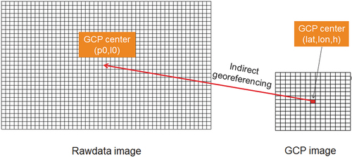
• For a given GCP image with the central pixel located at (latitude, longitude, and height), the corresponding image coordinates (l0, p0) on the frame image were obtained using the initial instrument line of sight model (see Figure 6). This step is performed using the indirect georeferencing approach. The image coordinates (l0, p0) represent the predicted GCP (line; pixel) in sensor geometry.

  Figure 6. GCP location in the raw data.

  

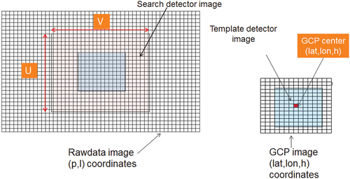
• Define an N×M area in the sensor geometry space around (l0, p0). For each element/pixel (li, pi) in the defined NxM detector, reconstruct the resampled value from the GCP image using a bi-cubic resampling method. The result is an N × M template detector image.

• A search detector image (U×V) around the template detector image is defined (see Figure 7), and a template matching procedure (via normalized cross-correlation) is applied to compute the observed GCP (line, pixel) in the sensor geometry. The GCP template detector image is moved in the horizontal and vertical directions inside the search window. The normalized cross correlation was calculated for each displacement position. The normalized correlation routine helps to remove any greyscale differences between the two images and to alleviate some of the problems with the different radiometric responses between the GCP chips extracted from the GLS2010 dataset (Landsat ETM+ sensor) and HyperScout-1 frames. A filtering of the outliers resulting from false template matching (for example, GCP images over cloudy areas) was performed based on a threshold on maximum correlation.

  Figure 7. GCPs template searching techniques.

  

5.3.4. Block bundle adjustment

GCPs identified in all HyperScout-1 successive frames (from the previous step) are then used in aerial triangulation, bundle block adjustment and camera calibration algorithms (Kornus, Lehner, and Schroeder 1999; Sima et al. 2016; Storey, Rengarajan, and Choate 2019). These steps were applied to estimate and refine the exterior orientations (satellite orientations) and the interiors orientation (focal plane distortion).

The image-based technique is a photogrammetric method for creating three-dimensional models of a feature or topography from overlapping two-dimensional photographs taken from many locations and orientations to reconstruct the photographed scene. Traditional photogrammetric methods require the 3-D location and pose of the camera(s) or the 3-D location of ground control points to be known to facilitate scene triangulation and reconstruction. In contrast, our approach solves the camera pose and scene geometry simultaneously and automatically by using a highly redundant bundle adjustment based on GCPs in multiple overlapping offset images. Precisely, it involves acquiring images from several positions relative to the object of interest. The GCPs identify distinctive features appearing in multiple images and establish the spatial relationships between the original camera positions in an arbitrary and unscaled coordinate system. A bundle adjustment was then used to calibrate the camera(s) and derive the geometric calibration parameters.

In the block bundle adjustment, the focal plan was modelled by a polynomial in x and y of 3^rd degree in both across and the along track direction (see the equation below). This focal plan model is common to all the frames. The exterior orientations are represented by a single set of roll, pitch, and yaw boresight angles for each acquired frame. Therefore, in total, the number of unknown parameters to be estimated in the bundle adjustment algorithm is equal to 10 polynomial coefficients × 2 (dy: along and dx: across) × 3 (boresight angles) ×number of acquired frames.

$\mathit{dx}=\mathit{a}\left(1\right)+\mathit{a}\left(2\right)\times \mathit{x}+\mathit{a}\left(3\right)\times \mathit{y}+\mathit{a}\left(4\right)\times x^2+\mathit{a}\left(5\right)\times \mathit{x}\times \mathit{y}+\mathit{a}\left(6\right)\times y^2+\mathit{a}\left(7\right)\times x^2\times \mathit{y}+\mathit{a}\left(8\right)\times \mathit{x}\times y^2+\mathit{a}\left(9\right)\times x^3+\mathit{a}\left(10\right)\times y^3$

$\mathit{dy}=\mathit{b}\left(1\right)+\mathit{b}\left(2\right)\times \mathit{x}+\mathit{b}\left(3\right)\times \mathit{y}+\mathit{b}\left(4\right)\times x^2+\mathit{b}\left(5\right)\times \mathit{x}\times \mathit{y}+\mathit{b}\left(6\right)\times y^2+\mathit{b}\left(7\right)\times x^2\times \mathit{y}+\mathit{b}\left(8\right)\times \mathit{x}\times y^2+\mathit{b}\left(9\right)\times x^3+\mathit{b}\left(10\right)\times y^3$

where:

x and y are the normalized pixels and lines, respectively.

a(1) to a(10) are the polynomial coefficients for the across track distortions dx.

b(1) to b(10) are the polynomial coefficients for the along track distortions dy.

GCPs measurements were used in the inversion process, and an outliers removal process was applied to detect and remove bad GCPs. The outlier removal step is based on an iterative procedure that eliminates GCPs with associated errors higher than three sigma. Covariance matrices were generated and analysed to quantify the variance of the estimated solution.

6. Level-1 inflight calibration results

6.1. Spectral calibration results

Spectral verification was carried out using the approach as explained in Section 5.1. The ‘20181107.02_Railroad_Valley’ image was used from the acquisitions listed in Table 3. The extent of the calibration site was manually delineated, all per pixel DN measurements of each spectral band were averaged and converted to radiances using the radiometric calibration model and coefficients established as described in Section 5.2. This is compared to the spectral radiances for the site and corresponding date derived from the spectral reflectances as provided by RadCalNet (CEOS). The RadCalNet data is sampled to 10nm, which nearly matches the 11 nm spectral sampling of Hyperscout-1.

The resulting spectral radiances are plotted in Figure 8. The spectral features appear to be well aligned between both spectra. We identified the three most prominent features visible in the spectrum (also indicated on in Figure 8), including a distinct feature around 760nm, corresponding to an oxygen absorption peak, often used for spectral calibration. We determined the location of the peaks using bicubic interpolation. Note that the accuracy of the peak locations is limited because of the fairly coarse spectral resolution of both the acquisition and reference spectrum. The locations of the peaks correspond very well, all within a 1nm margin (see Table 5). This indicates no significant spectral shifts were present, and therefore no spectral corrections were applied.

Figure 8. Spectral calibration: modelled and measured spectra with indication of spectral features (spectra scaled for viewing purposes).

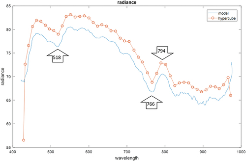
Table 5. HyperScout-1 spectral calibration results.

#feature	Measured wavelength [nm]	Modelled wavelength [nm]	Deviation [nm]
A	517.25	518.01	0.76
B	766.22	766.40	0.18
C	792.8	793.54	0.74

6.2. Radiometric calibration results

6.2.1. Verification of pre-flight absolute calibration coefficients

During the pre-flight instrument characterization campaign, a set of absolute calibration parameters was determined. To verify their validity, we apply the radiometric model using the parameters to convert a raw DN image to radiances. Next, we calculate modelled radiances using the OSCAR model, for the matching acquisition location time, viewing, illumination and atmospheric conditions.

We used the ‘20181107.01_Libya4’ image, delineate a suitable region manually, computed average radiances and plotted it in Figure 9. In the same figure, we also plotted the modelled radiances for the same area, both the direct output of the model, and a version in which the spectrum is convolved with the spectral responses of the HyperScout-1 instrument.

Figure 9. Radiances for the ‘20181107.01_Libya4’ site: blue) generated using the OSCAR model, orange) with HyperScout-1 spectral responses applied, yellow) HyperScout-1 results with pre-flight calibration.

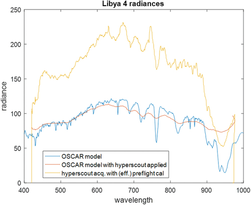
The results show a major discrepancy between the spectra, indicating that the pre-flight calibration does not provide a useable absolute calibration. This confirms the need for performing inflight absolute calibration.

6.2.2. Inflight determination of new absolute calibration coefficients

The spectral radiances as plotted in Figure 9 do not only illustrate the need for inflight calibration but also contain all necessary information to determine new calibration coefficients ($A_{in\mathrm{flight}}^K$). As outlined in section 5.2.2, a new set of inflight calibration coefficients ($A_{in\mathrm{flight}}^K$) can be derived by using the radiances of the OSCAR model ($L_{mo\mathrm{del}}^k)$, together with the radiances calculated from the acquisition. When using the new calibration coefficients to calculate radiances from the acquisition, an exact correspondence is obtained to the modelled radiances:

$L_{in\mathrm{flight}}^k=A_{in\mathrm{flight}}^K\ast \mathit{D}{N}_{acq}^K$ = ($\frac{L_{m\mathrm{odel}}^K}{L_{p\mathrm{reflight}}^K}{A}_{pr\mathrm{eflight}}^K)\ast \mathit{D}{N}_{acq}^K=L_{mo\mathrm{del}}^K$

We calculated $L_{in\mathrm{flight}}^k$ for the ‘20181107.01_Libya4’ site using the newly derived $A_{in\mathrm{flight}}^K$. They exactly matched the modelled radiances $L_{mo\mathrm{del}}^k$, confirming the correctness of the calculation.

6.2.3. Line based vs band-based calibration

Initially, we performed the absolute calibration band per band, hereby pooling the statistics of 36 adjacent lines together to generate calibration coefficients per band. This however leads to unacceptable artefacts. This is shown in Figure 10 (left): strong banding is visible at the transition between bands. Therefore, we switched to an approach in which each sensor line is treated as a separate band, for which a separate absolute calibration coefficient is determined. The result of this is shown in Figure 10 (right): the striping artefacts are resolved nearly completely.

Figure 10. ‘20181107.02_Railroad_Valley’ image, corrected with results of left: band-based calibration, right: line based calibration.

It has to be noted that even with perfect line-based calibration, some striping can still occur when imaging locations for which the real shape of the spectrum contains sharp slopes. Since each line has a slightly different spectral response, it produces a different result for such sloped spectrum. Pooling the results of 36 lines together into a single spectral band which shows variations corresponding to the lines, even for uniform regions. This issue cannot be resolved by the calibration but is an inherent limitation of the instrument concept.

6.2.4. Verification of inflight absolute calibration coefficients

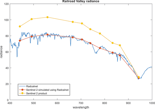
To validate the inflight absolute calibration parameters, we applied them to an acquisition which is independent of the one on which the calibration itself was based. For this, we used the ‘20181107.02_Railroad_Valley’ image. A suitable region was manually delineated, and statistics were collected for all image lines. Since the site is quite small, the number of pixels per line that could be used was limited, so the result per line also has limited accuracy. Next, we converted them to radiances using the radiometric model and plotted them in Figure 12. The small variations in the radiance spectrum are due to inaccuracies at line level, they are averaged out at the spectral bands level. Independently, a radiance spectrum was obtained for the same site from RadCalNet, using the matching acquisition time, viewing, illumination and atmospheric conditions.

As discussed in Section 5.2.2, there are strong indications that radiances obtained from RadCalNet might be biased (Sterckx and Wolters 2019). To eliminate such bias, additional correction step was performed. We looked up a closely matching Sentinel-2 acquisition and collected radiances for its multispectral bands, using the same area. We derived the RadCalNet model for the matching conditions and resampled it to the Sentinel-2 spectral responses. Both are plotted in Figure 11. Assuming correct absolute radiances in the real Sentinel-2 product, the bias in the RadCalNet results is obvious: over the spectral range considered, its radiance values are about 14% lower. We, therefore, applied a correction to the modelled values to compensate this.

Figure 11. Radiances for Railroad Valley site using sentinel-2 multispectral bands.

Results are shown in Figure 12. We plotted bias-corrected radiances obtained from RadCalNet and compared them to radiances obtained from the ‘20181107.02_Railroad_Valley’ acquisition, converted to spectral radiances using the inflight calibration parameters.

Figure 12. Radiances for the Railroad Valley site using the (corrected) RadCalNet model, and derived from the hyperscout-1 acquisition and inflight calibration parameters.

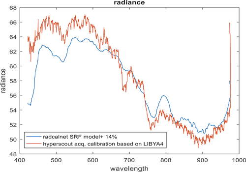
Both, the overall radiance levels, and the spectral shape match well. Even including the variations from line to line, the differences in radiance are well below 5%. This is an encouraging result, even if the extremely limited number of calibration acquisitions does not allow to make a more detailed comparison including error estimates.

6.2.5. Independent assessment of radiometric quality

The radiometric quality of the HyperScout-1 mission was also independently verified by the ESA Earthnet Data Assessment Project (EDAP) (Lavender 2022). Radiometric calibration assessment was performed by comparing the reflectance derived from the ‘20181107.02_Railroad_Valley’ image with corresponding reflectances from RadCalNet data, including appropriate BRDF correction. The comparison was performed on a 1kmx1km square (much smaller area than the one used during calibration).

The assessment results showed a close correspondence between the HyperScout-1 and RadCalNet data, with differences smaller than 10% across matching bands. The bulk of the difference can be attributed to BRDF effects: the HyperScout-1 data was assumed to be nadir-viewing.

These results cannot be considered as a true independent verification, as the same image was used in the calibration process but it still demonstrates the validity of the approach.

6.3. Geometric calibration results

6.3.1. Assessment of the initial geometric accuracy

6.3.1.1. Initial absolute geolocation

After the HyperScout-1 launch and before performing any calibration activities, it is important to assess the absolute geolocation accuracy obtained by relying solely on the provided telemetry (satellite positions and attitudes) together with the pre-flight measured line of sight. This analysis allowed us to estimate the initial absolute geolocation bias and to apply a coarse boresight correction to reduce the geolocation error to a reasonable value. To this end, manual GCPs were selected for each Region of Interest (ROI) and used to estimate the correction to be applied.

This section provides an overview of the results and analysis of the HyperScout-1 initial performance using the pre-flight calibration parameters (measured before launch). These parameters include the line of sight model of the subsampled pixels of the 2D sensors expressed in the sensor frame. The satellite boresight verification steps were performed, and an initial absolute geolocation performance was assessed. This assessment showed a large bias for all the processed ROIs. This bias differs from one ROI to another with the lowest measured bias of 26.4 km for the ‘20181031_Ceylanpinar’ ROI and the maximum bias of 183 km for the ‘20181120_Bahamas’ ROI (see Table 6). These large biases are related to time mis-synchronization issues between the platform and instrument. Table 6 shows the result of the initial absolute geolocation assessment for each ROI, together with a map showing the projected HyperScout-1 frame overlaid with Google Earth images of the same areas.

Table 6. Initial absolute geolocation errors for all processed ROIs.

ROI	Footprint	Geolocation errors
20181108.01_Algeria		bias of ~58 km
20181107.02_Railroad_Valley		bias of ~73 km
20181031_ceylanpinar		bias of ~26.4 km
20181120_bahamas		bias of ~183 km

6.3.1.2. Initial frame mis-registration errors

In addition to the large absolute geometric bias observed for all ROIs, we also noticed a frame co-registration issue (see Figures 13 and Figure 14). The projected frame is not well superimposed with respect to each other’s (e.g. 6 pixels shift between frame#1 and frame#2 see Figure 13). The shift increases with the increase in the time separation between the frames. This issue is very major as it has a significant impact when building the spectral bands from the frames. This was caused by inaccurate attitudes or satellite positioning. However, during the commissioning, these issues were corrected for by varying the satellite boresight angles w.r.t time to account for the increasing shift.

Figure 13. Observed shift between successive frames. The image is a false colour RGB image (R: projected frame#1, G: projected frame#2, and B: projected frame#2).

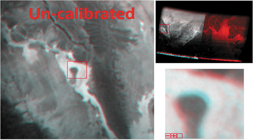
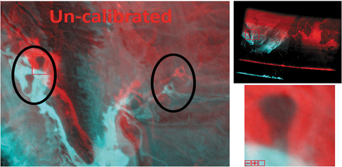
Figure 14. Observed shift between further away frames. The image is a false colour RGB image (R: projected frame#1, G: projected frame#15, and B: projected frame#15).

6.3.1.3. Measured focal plane distortions

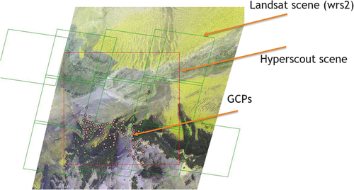
The boresight coarse correction (see section 5.3.2) was applied improving the absolute geolocation accuracy of all acquisitions close to the true location with a residual bias from 300 m to 1.5 km. This reduction in the overall absolute error allowed us to apply the GCP processing step then in order to estimate the initial focal plane distortions. The estimation is based on an automatic GCP selection and matching using the Global GCP dataset available from the Landsat Global Land Survey GLS 2010 (Figure 15). GCPs are located entirely in the bottom half of the HyperScout-1 scene (Figure 15). This is not a mal function of the GCPs selection process but rather linked to the arrangement of the focal plane layout where almost half of the CMV12000 sensor was used for imaging (illuminated frame in Figure 4).

Figure 15. Illustration of the GCP selection performed for the ‘20181108.01_Algeria’ site. The GCPs were extracted from the Landsat global land survey CGP database (see section 5.3.1). The green areas are the Landsat scenes intersecting with the HyperScout-1 ROI bounding box.

To characterize the distortion over the entire field of view, the ‘20181108.01_Algeria’ site is selected since it was acquired using the full frame acquisition mode and covers the full swath. The GCP processing step was applied for each single frame and estimated the across and along track distortion for each GCP sample. Note that due to acquisition’s choices applied to ‘20181108.01_Algeria’ to limit the data downlinked, the frames 1, 4, 7, 10 and 13, were acquired with full swath while the rest is acquired with half of the swath. Therefore, for the frames that cover half of the swath, it was not possible to estimate the distortions all over the entire swath.

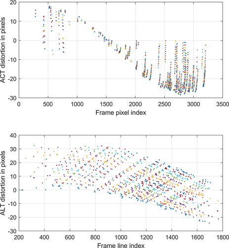
The distortions measured during the commissioning phase showed an actual focal plane layout quite different from the expected one (see Figure 16). The across track distortion is symmetric w.r.t to the centre of the swath with ± 20 pixels measured at the edge of the swath. This across track distortion is common to all frames and thus a single correction can be applied to all frames. Note that outliers are observed due to false GCP matching and were discarded in the correction process. However, the along track distortion showed a gradual increase of the distortion (from 0 to +30 pixels) when comparing the different frames. This suggests that there is systematic on-ground shift of about 3 to 5 pixels between the frames. This finding is also visible in Figure 13 (a false RGB image, R: projected frame#1, G: projected frame#2, and B: projected frame#2). This systematic shift was not expected to happen within a short-time acquisition (1/3 of second).

Figure 16. Measured initial focal plane distortion in across track (top) and along track (bottom) direction observed for all frame acquired above the ‘20181108.01_Algeria’ site. Each dot is representing a GCP distortion measurement and each colour is representing a frame (in total 15 frames were processed).

6.3.2. Block bundle adjustment results

Block Bundle adjustment was applied to all frames of the ’20181108.01_Algeria’ frame. In total 15 frames were used and allowed the estimation of the focal plane correction parameters (common to all frames) and a set of boresight angles for each frame.

Table 7 and Figure 17 summarize the results before and after applying the block bundle adjustment for all processed frames. A significant reduction in the across and along track distortion errors is observed for all frames and GCPs. The average absolute geolocation is estimated within sub-pixel (~0.48 pixels in across track and 0.51 pixels in along track).

Figure 17. Geometric absolute error (top: across track; bottom: along track). Green points show the error before calibration and the black points show the error after calibration.

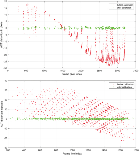
Table 7. Table showing per frame, the geometric error in across and along track (in pixels) before and after the calibration.

	Average Across track error (pixel)	Average Along track error (pixel)	Average Across track error (pixel)	Average Along track error (pixel)
	Before calibration		After calibration
Frame 1	13,36	10,06	0,48	0,48
Frame 2	16,28	8,22	0,50	0,47
Frame 3	16,92	7,90	0,51	0,43
Frame 4	14,32	8,41	0,50	0,51
Frame 5	17,35	7,56	0,49	0,51
Frame 6	17,36	8,86	0,46	0,54
Frame 7	15,50	10,29	0,51	0,54
Frame 8	18,61	11,36	0,47	0,44
Frame 9	18,77	13,11	0,49	0,48
Frame 10	15,92	15,42	0,52	0,51
Frame 11	19,09	16,96	0,46	0,51
Frame 12	20,33	17,38	0,43	0,53
Frame 13	18,15	18,59	0,54	0,61
Frame 14	21,76	18,69	0,38	0,59
Frame 15	22,99	16,83	0,43	0,48

7. Conclusion

In summary, HyperScout-1 satellite is an In-orbit Demonstration (IOD) mission carrying a miniaturized hyperspectral instrument built based on Linear Variable Filter hyperspectral technology. The calibration of such payload, during its flight is an important achievement allowing better characterization and understanding of such novel Earth observation technique onboard CubeSat platform. This calibration process is crucial to ensure the accuracy and dependability of the data collected by the satellite. The quality of research and applications that rely on this data greatly benefit from it.

Through a radiometric calibration procedure, we have successfully identified and minimized various sources of radiometric error including spectral shifts and absolute variations. As a result, the HyperScout-1 instrument now performs with improved accuracy (less 5%) and consistency in measuring Earth surface properties.

The main limitation for calibration of the HyperScout-1 mission is its extremely limited data budget. This had an important impact on the radiometric calibration strategy. Typically, regular observations over well-selected sites are needed accurately calibrate the instrument radiometric behaviour. A trade-off had to be made to reach the best possible radiometric accuracy given the limited amount of imagery. Still, we were able to calibrate the HyperScout-1 instrument and demonstrated the capability of such Linear Variable Hyperspectral technology onboard CubeSats platforms to deliver good-quality imagery.

Additionally, our efforts in calibration have effectively addressed challenges related to sensor orientation, distortion and georeferencing. This has significantly enhanced the accuracy of the collected data allowing for quality orthorectified imagery generation and geospatial product development. The average absolute geolocation is estimated within sub-pixel (~0.48 pixels in across track and 0.51 pixels in along track). These improvements are crucial for applications like land cover classification, change detection and disaster monitoring.

It is important to note that inflight calibration in general is a process that requires repeated efforts over the lifetime of a mission. The results shared in this paper provide a snapshot of the satellite’s performance at one moment in time. Due to the short HyperScout-1 lifetime, it was not possible to regularly update the calibration parameters. However for longer missions, it is crucial to update and validate the calibration of data on a regular basis to ensure its accuracy and reliability throughout the mission duration.

The successful calibration of HyperScout-1 not only contributes to our understanding of Earth’s dynamic processes but also paves the way for improved and affordable hyperspectral data from SmallSats supporting decision-making in various fields, such as agriculture, forestry, environmental monitoring, and disaster management. Moreover, the insights gained from this calibration process can inform future SmallSats missions and inspire advancements in remote sensing technology. The crucial takeaway for future missions with similar characteristics is to increase downlink capacity significantly. Doing so would enhance mission utility by enabling the production of not only more, but also higher-quality images.

Acknowledgements

The authors thank the HyperScout-1 consortium: Cosine Measurement Systems B.V (Netherlands), the ESA GSTP (General Supporting Technology Program) team, S[&]T AS (Norway), TU-Delft (Netherlands) and VDL (Netherlands).

Disclosure statement

No potential conflict of interest was reported by the author(s).

Additional information

Funding

This work was supported by the European Space Agency [4000117882/16/NL/PS/gp].

References

- AMS. 2022. CMV12000 12Mp High Speed Machine Vision Global Shutter CMOS Image Sensor (Datasheet) Vol. DS00060. v5-00 84. AMS OSRAM Group
- Bo-Cai Gao, K. M., P. Yang, and P. Yang. 2004. “A New Concept on Remote Sensing of Cirrus Optical Depth and Effective Ice Particle Size Using Strong Water Vapor Absorption Channels Near 1.38 and 1.88/Spl Mu/M.” IEEE Transactions on Geoscience and Remote Sensing 42 (9): 1891–1899. https://doi.org/10.1109/TGRS.2004.833778.
- Cogliati S., F. Sarti, L. Chiarantini, M. Cosi, R. Lorusso, E. Lopinto, F. Miglietta, et al. (2021). The PRISMA imaging spectroscopy mission: overview and first performance analysis. Remote Sensing of Environment, 262: 112499. https://doi.org/10.1016/j.rse.2021.112499
- Esposito, M., S. S. Conticello, N. Vercruyssen, C. N. Van Dijk, P. F. Manzillo, B. Delauré, I. Benhadj, et al. 2018. “Demonstration in Space of a Smart Hyperspectral Imager for Nanosatellites.” In 32nd Annual AIAA/USU Conference on Small Satellites.
- Esposito, M., and A. Z. Marchi. 2015. “HyperCube the Intelligent Hyperspectral Imager.” In 2015 IEEE Metrology for Aerospace (MetroAeroSpace), 547–550. Benevento, Italy: IEEE. https://doi.org/10.1109/MetroAeroSpace.2015.7180716.
- Esposito, M., and A. Z. Marchi. 2019. “In-Orbit Demonstration of the First Hyperspectral Imager for Nanosatellites.” In International Conference on Space Optics — ICSO 2018, edited by N. Karafolas, Z. Sodnik, and B. Cugny, 71. Chania, Greece: SPIE. https://doi.org/10.1117/12.2535991.
- Govaerts, Y., S. Sterckx, and S. Adriaensen. 2013. “Use of Simulated Reflectances Over Bright Desert Target As an Absolute Calibration Reference.” Remote Sensing Letters 4 (June): 523–531. https://doi.org/10.1080/2150704X.2013.764026.
- Guanter, L., H. Kaufmann, K. Segl, S. Foerster, C. Rogass, S. Chabrillat, T. Kuester, et al 2015. “The EnMAP Spaceborne Imaging Spectroscopy Mission for Earth Observation.” Remote Sensing 7 (7): 8830–8857. https://doi.org/10.3390/rs70708830.
- Guanter, L., R. Richter, and J. Moreno. 2006. “Spectral Calibration of Hyperspectral Imagery Using Atmospheric Absorption Features.” Applied Optics 45 (10): 2360. https://doi.org/10.1364/AO.45.002360.
- Hagen, N. 2012. “Snapshot Advantage: A Review of the Light Collection Improvement for Parallel High-Dimensional Measurement Systems.” Optical Engineering 51 (11): 111702. https://doi.org/10.1117/1.OE.51.11.111702.
- Hueni, A., J. Biesemans, K. Meuleman, F. Dell’endice, D. Schlapfer, D. Odermatt, M. Kneubuehler, et al. 2009. “Structure, Components, and Interfaces of the Airborne Prism Experiment (APEX) Processing and Archiving Facility.” IEEE Transactions on Geoscience & Remote Sensing 47 (1): 29–43. https://doi.org/10.1109/TGRS.2008.2005828.
- Itten K., F. Dell’Endice, A. Hueni, M. Kneubühler, D. Schläpfer, D. Odermatt, and F. Seidel. 2008. APEX - the Hyperspectral ESA Airborne Prism Experiment. Sensors 8 (10): 6235–6259. https://doi.org/10.3390/s8106235
- Kornus, W., M. Lehner, and M. Schroeder. 1999. “Geometric Inflight-Calibration by Block Adjustment Using Moms-2p-Imagery of Three Intersecting Stereo-Strips.” In ISPRS Workshop on Sensors and Mapping from Space.
- Lavender, S. 2022. “Technical Note on Quality Assessment for GomX-4B HyperScout-1.” Issue 1, ESA EDAP.REP.042.
- Leon, P. L., and P. Koch. 2018. “GOMX-4 - the Twin European Mission for IOD Purposes.” In 32nd Annual AIAA/USU Conference on Small Satellites.
- Liu, P., J. Pei, H. Guo, H. Tian, H. Fang, and L. Wang. 2022. “Evaluating the Accuracy and Spatial Agreement of Five Global Land Cover Datasets in the Ecologically Vulnerable South China Karst.” Remote Sensing 14 (13): 3090. https://doi.org/10.3390/rs14133090.
- Livens, S., B. Delauré, A. Lambrechts, and N. Tack. 2014. “Hyperspectral Imager Development Using Direct Deposition of Interference Filters.” In 4S Symposium. Porto Petro, Majorca, spain.
- Macleod, H. A. 2003. Thin-Film Optical Filters. 3. ed., repr ed. Bristol: Institute of Physics.
- Maresi, L., M. Taccola, M. Kohling, and S. Lievens. 2010. “PhytoMapper – Compact Hyperspectral Wide Field of View Instrument.” In Small Satellite Missions for Earth Observation, edited by R. Sandau, H.-P. Roeser, and A. Valenzuela, 321–330. Berlin, Heidelberg: Springer. https://doi.org/10.1007/978-3-642-03501-2_30.
- Moreau, D. C., G. Lousberg, L. Maresi, and B. Delauré. 2012. “Development of a Compact Hyperspectral/Panchromatic Imager for Management of Natural Resources.” In Small Satellites Systems and Services. Portoroz, Slovenia.
- Riazanoff. 2004. “SPOT 123-4-5 Satellite Geometry Handbook.” GAEL-P135-DOC-001, 1: 82
- Shen-En, Q. 2020. Hyperspectral Satellites and System Design. 1st ed. CRC Press. https://www.routledge.com/Hyperspectral-Satellites-and-System-Design/Qian/p/book/9780367217907#.
- Sima, A. A., P. Baeck, D. Nuyts, S. Delalieux, S. Livens, J. Blommaert, B. Delauré, and M. Boonen. 2016. “Compact Hyperspectral Imaging System (Cosi) for Small Remotely Piloted Aircraft Systems (Rpas) – System Overview and First Performance Evaluation Results.” ISPRS - International Archives of the Photogrammetry Remote Sensing and Spatial Information Sciences XLI-B1 (June): 1157–1164. https://doi.org/10.5194/isprsarchives-XLI-B1-1157-2016.
- Soukup, M., J. Gailis, D. Fantin, A. Jochemsen, C. Aas, P. J. Baeck, I. Benhadj, et al. 2016. “HyperScout: Onboard Processing of Hyperspectral Imaging Data on a Nanosatellite.” In The 4S Symposium.
- Sterckx, S., I. Benhadj, G. Duhoux, S. Livens, W. Dierckx, E. Goor, S. Adriaensen, et al. 2014. “The PROBA-V Mission: Image Processing and Calibration.” International Journal of Remote Sensing 35 (7): 2565–2588. https://doi.org/10.1080/01431161.2014.883094.
- Sterckx, S., and E. Wolters. 2019. “Radiometric Top-Of-Atmosphere Reflectance Consistency Assessment for Landsat 8/OLI, Sentinel-2/MSI, PROBA-V, and DEIMOS-1 Over Libya-4 and RadCalnet Calibration Sites.” Remote Sensing 11 (19): 2253. https://doi.org/10.3390/rs11192253.
- Storey, J. C., R. Rengarajan, and M. J. Choate. 2019. “Bundle Adjustment Using Space-Based Triangulation Method for Improving the Landsat Global Ground Reference.” Remote Sensing 11 (14): 1640. https://doi.org/10.3390/rs11141640.
- Zuccaro, M. A., A. Deep, and S. Grabarnik. 2012. “Μtma – a Miniaturised Hyperspectral for CubeSat.” In The 4S Symposium. Portorož, Slovenia.