Comparative analysis of multispectral data between GF-1 WFV4 and GF-6 WFV sensors

ABSTRACT

In recent years, China has launched a number of Gaofen (GF) series earth observation satellites. It is crucial to understand the relationship between the data of the GF series of satellite sensors for the selection of sensor images for scientific research. Taking the same-day transit image pairs of three regions as the study data, this paper compares the consistency of the Top of Atmosphere (TOA) reflectance of GF-1 WFV4 and GF-6 WFV sensors by using the TOA mean comparison method, and discusses the differences in water body and vegetation extraction. The results indicate that the satellite signal intensity in different land cover types and areas differs significantly. In the bare soil-dominated region, GF-1 WFV4 has a larger signal strength than GF-6 WFV, while in the vegetation-dominated region, it turns out to be just the opposite. The difference between the two sensors is mainly related to the difference in the spectral response function and the radiometric resolution of the two satellites. In addition, the determination coefficient (R²) of the corresponding bands of the two sensors is all greater than 0.90, indicating that the two sensors have strong linear correlation and good complementarity.

KEYWORDS:

• GF-1 WFV4
• GF-6 WFV
• comparative analysis
• top of Atmosphere (TOA) reflectance

1. Introduction

As an important data source for geographic information analysis, satellite remote-sensing images made important contributions in environmental monitoring, urban planning, resource utilization and so on. In recent years, with the increase in the number and types of satellites, it has become possible to carry out all-hours and all-weather earth observation, and it has become a trend to comprehensively use multi-source remote sensing images to conduct scientific research and monitor global resources and environmental changes (Camps-Valls et al. 2008; Shan et al. 2019). However, due to the limitation of the sensor’s own design, the satellite signals it transmits will fade over time (Chander, Meyer, and Helder 2004), and the coverage of the acquired remote sensing images will be limited. This results in the phenomenon that for the same area, remote sensing images acquired by satellite sensors of different platforms have different consistency of data radiometry due to the influence of the sensor’s own conditions such as orbital altitude, orbital inclination, revisit period, or other external conditions such as acquisition time, terrain relief, atmospheric conditions, lighting conditions, etc. (X. Chen, Lee and Don 2005). In practical applications, image stitching (Zhang et al. 2017) is often used to obtain a wide range of images for research purposes. In the face of many satellite age date, how to make full use of the complementarity between heterogeneous satellite remote sensing images, eliminate the influence of ‘non-geomorphic factors’ (Zhong, Bian and Li 2018) and judge the differences between sensors (Song et al. 2021), it is the premise of comprehensive utilization of multiple source remote sensing data.

At present, the study of interaction comparison between sensor data is more common in the field of remote sensing, which is a hot research topic in the field of remote sensing. Many scholars have carried out the study of interaction comparison between different types of sensor data of the same series and different types of sensor data of different series. Interactive comparison between synchronous image pairs of different sensors is also called interactive calibration, which aims to quantitatively evaluate the relationship between two sensors (Teillet et al. 2001; H. X. Xu, Zhang, and Li 2011). The methods of cross-calibration can be divided into those based on comparisons between corresponding bands and those based on indices (H. X. Xu, Zhang, and Li 2011). The former is a correlation analysis of data from the same or similar bands between two sensors, and the method directly reflects the interrelationship between the bands; the latter studies the difference of signal intensity of sensors to different features by constructing index of common bands between sensors. It has been 50 years since the launch of Landsat-1 in 1972, and many satellites in the series have been launched. The series has been updated to Landsat-9, and because of the open source and availability of its sensor data, it is common for domestic and foreign scholars to study the interactive comparison of sensor data Landsat series satellites (Li, Jiang and Feng 2014; Mishra et al. 2014; Roy et al. 2016; She et al. 2015; Vogelmann et al. 2001). Due to the high calibration accuracy of Landsat series satellites, cross-comparison studies between Landsat satellite sensor data and other satellite sensor data such as IRS-P6 (Chander, Coan, and Scaramuzza 2008), EO-1 ALI (Camps-Valls et al. 2008) and Sentinel (Padró et al. 2017; G. Xu and Xu 2021; Y. Xu et al. 2018; Zhong, Bian, and Li 2018) are also common. With the rapid development of remote sensing technology, remote sensing image data have shown the ‘three high’ characteristics of high spatial, high spectral and high temporal resolution, and the comparison of medium resolution satellite sensor data with high-resolution satellite sensor data IKONOS (Goward et al. 2003), GF-1 (Zhao et al. 2020), GF-4 (Y. Chen et al. 2017), etc., as well as the comparisons between high-resolution satellite sensor data (H. Xu, Sun, and Xu 2021). Synthesizing the existing studies, the interactive comparison between synchronous image pairs of different sensors can be roughly divided into two categories, one is the calibration of an unknown sensor with known sensor (Vogelmann et al. 2001), and the other is the interactive comparison between data of two sensors that has been calibrated (Sun, Feng, and Xu 2012). This cross-comparison method of synchronous image pairs among sensors reflects the differences of sensor characteristics, apparent reflectance and spectral features. The cross-comparison method compares observations from multiple sensors or the same sensor at different times to eliminate inter-sensor systematic differences, thereby enhancing data consistency and reliability. This approach establishes robust relationships between different sensors, enabling mutual validation and calibration of data without requiring complex ground observation equipment. It offers broader applicability and lower costs compared to traditional methods.

With the continuous development of China’s space industry, China has also successfully launched various types of satellites such as resource satellites (ZY), Gaofen series satellites (GF), and environmental satellites (HJ), and since then the interactive comparison studies of domestic satellite sensor data has gradually increased. For example, Wang et al. (2015) compared the differences of sensors by comparing GF-1/WFV, ZY-3/MUX and HJ-1/CCD in terms of vegetation cover, leaf area index (LAI), NDVI, etc. The results showed that the sensors differed in estimated coverage performance, and the influence of zenith angle change on reflectance and NDVI is greater than that of spectral response function. Wu et al. (2020) discussed the apparent reflectance consistency relationship between GF-1, GF-2 and Landsat8 and found that the reflectance of the two domestic satellites is more consistent, while there were differences with Landsat8 and proposed a conversion model to reduce such differences. Xu et al. (2021) compared the hyperspectral AHSI and multispectral VIMI sensor data of the GF-5 satellite and found that although both sensors were on the same satellite, their irradiance data also had a certain deviation, with a deviation rate close to 32%. Ye et al. (2021) cross-calibrated the VIMS and TIR of HMS5 and found that the calibrated LST and brightness temperature were significantly improved and the LST retrieval error was greatly reduced. On 6 November 2019, the China National Space Administration opened free access to the image data of GF-1 and GF-6 with a spatial resolution of 16 m to the world.

At present, comparative studies of the interaction between the GF series of satellites and other sensors are more common, but the interactive comparison between GF-1 WFV4 and GF-6 WFV sensor data is rarely reported. It is also unclear whether the two sensor data can be used in concert and how the two sensors relate to each other. In this paper, three groups of same-day transit image pairs are used to compare and analyse the relationship between the two sensors and to determine the relationship equation between the two conversions so that the two sensor data can complement each other in practical applications, and further broaden their application fields.

2. Study area data and preprocessing

2.1. Study area data

GF-6 is the follow-up satellite of GF-1. They are all solar synchronous satellites with a very similar imaging system, and both have the same satellite revisit period, orbital inclination, coverage period, regression cycle, etc. (Table 1). The GF-1 WFV4 multispectral camera has four bands of blue, green, red, and near infrared (NIR). Its spatial resolution is 16 m, the swath width is 200 km, and the radiometric resolution is 10 bit. The GF-6 WFV multispectral camera with a spatial resolution of 16 m has eight bands, and the bands of blue, green, red and NIR have the same spectral range as GF-1 WFV4. Its swath width is 800 km, and the radiometric resolution is 12 bit. In terms of sensor band setting, GF-1 WFV4 and GF-6 WFV satellite sensors both set the blue (B1), green (B2), red (B3) and NIR band (B4) with the same spectral range (Table 2).

Table 1. GF-1 WFV4 and GF-6 WFV satellite orbit parameters.

parameter	GF-1 WFV4	GF-6 WFV
Orbit type	Sun synchronous orbit	Sun synchronous orbit
Revisitation period/d	4	4
Orbital altitude	645 km	644.5472 km
Orbit inclination	98.0506º	97.9597°
Local time of descending node	10:30 AM	10:30 AM
Return to the circle times	605	605
Return period	41 Day	41 Day

Table 2. GF-1 WFV4 and GF-6 WFV satellite sensor parameters.

Parameter		GF-1 WFV4	GF-6 WFV
Launch time		2013/4/26	2018/6/2
Camera type		Wide field of view camera (WFV)	Wide field of view camera (WFV)
Radiometric resolution/bit		10	12
Spatial resolution/m		16	16
Width/km		200	800
Spectral range/μm	B1	0.45–0.52	0.45–0.52
	B2	0.52–0.59	0.52–0.59
	B3	0.63–0.69	0.63–0.69
	B4	0.77–0.89	0.77–0.89

The two sensors GF-1 GFV4 and GF-6 WFV have a few areas of overlapping images in the same daytime, and the range of overlapping areas is also very small. Considering the consistency of the feature spectra of different sensor data, this paper selects the data of three same-day transit image pairs from three different study areas as the data source for the comparative study of sensor data. The six remote sensing images are the image pairs of the Bortala Mongolia region in Xinjiang on 6 November 2020, the Changji region in Xinjiang on 25 July 2020 and the Hohhot region in Inner Mongolia on 9 November 2020. The location and size of the image pairs for the three regions are presented in Table 3. The image pairs of the Bortala Mongolia region and the Changji region are selected as experimental data, and the distribution types of ground objects in these two regions are mainly bare soil and vegetation, respectively. The image pairs of the Hohhot region, which is rich in surface types, are used as validation data to verify the experimental results (Figure 1). The selected image pairs in different regions are transited on the same day, with the same external conditions and land cover types. The insolation and atmospheric conditions of each pair of synchronized images are good, and the solar zenith angle and solar azimuth angle are close to each other (Table 4), thus ensuring the consistency of earth observations by different sensors and avoiding the randomness of experimental results.

Figure 1. GF-1 WFV4 (a–c) vs. GF-6 WFV (e–f) image pairs (RGB: 432). (a)–(c) show the GF-1 WFV4 data for the three regions, (d)–(f) show the GF-6 WFV data for the three regions.

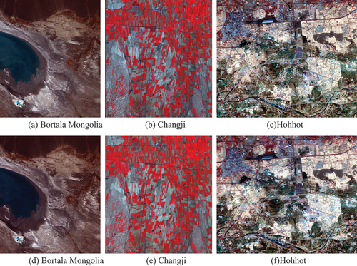
Table 3. The location and size of the image pairs in the study area.

Study area	Latitude	Longitude	pixel numbers
Bortala Mongolia	44°39′59”−45°3′21“N	82°56′38”−83°24′52“E	2659×2272
Changji	43°45’29”−43°57′43“N	89°26′38“−89°42′08” E	1383×1260
Hohhot	40°26′00”−40°35′59“N	110°29′16”−110°44′56“E	1384×1161

Table 4. The parameters of the synchronizing image pairs.

Image pairs	Sensor	date	Time	Solar zenith (°)	Solar azimuth (°)	Satellite zenith (°)	Satellite Azimuth(°)	Roll satellite angle (°)
Bortala Mongolia	GF1-WFV4	2020/11/06	14:00:32	61.15	175.41	35.66	286.75	7.999
	GF6-WFV		13:32:18	61.44	175.09	6.33	25.63	−0.003
Changji	GF1-WFV4	2020/07/25	13:30:12	25.50	155.88	26.60	285.88	0.000
	GF6-WFV		12:56:19	25.15	151.21	12.97	72.06	−8.993
Hohhot	GF1-WFV4	2020/11/09	11:58:02	57.47	171.62	26.59	285.18	0.000
	GF6-WFV		11:29:58	57.47	171.97	12.99	71.85	−9.005

2.2. Data preprocessing

The preprocessing of GF-1 and GF-6 data mainly includes ortho-correction, radiometric correction, alignment, cropping, etc. Due to terrain fluctuations, sensor settings and other factors, the geometric distortion of GF-1 WFV4 and GF-6 WFV is different, so it is necessary to eliminate the error caused by geometric distortion through orthography correction. Firstly, ortho-correction is performed by using the file of Rational Polynomial Coefficient (RPC) provided by the China Resource Satellite Applications Center to reduce the data error caused by geometric distortion. Then, one of the scene images is used as the reference image to perform geometric correction on other images. Finally, radiation correction is conducted on the corrected images to reduce the radiation distortion or error caused by the sensor’s own conditions, atmospheric conditions, illumination conditions and some noises during the imaging process. It can be seen from Table 4 that the maximum transit time difference between the image pairs used is 34 min. In this study, the effects of ground and atmospheric conditions caused by this time difference are ignored, and the Illumination Correction Model (ICM) (Chander, Markham and Helder 2009) is used for radiometric correction (Eq. (2)(2) ${\rho }_{\lambda }=\frac{\mathit{\pi }\times {\mathit{L}}_{\mathit{\lambda }}\times d^2}{cos{\theta }_{\mathrm{z}}(\mathit{ESU}{N}_{\mathit{\lambda }}\times cos{\theta }_{\mathrm{s}})}$(2) ). For the given GF-1 WFV4 and GF-6 WFV data, the corresponding apparent reflectance is calculated as follows. First, the original image pixels are converted into corresponding radiance values (Eq. (1))(1) $L_{\lambda }=Q_{\lambda }\times \mathit{G}\mathrm{ai}{\mathrm{n}}_{\lambda }+\mathrm{Bia}{\mathrm{s}}_{\lambda }$(1) to eliminate errors generated by the sensor. The radiance values are then converted into apparent reflectance (Eq. (2)(2) ${\rho }_{\lambda }=\frac{\mathit{\pi }\times {\mathit{L}}_{\mathit{\lambda }}\times d^2}{cos{\theta }_{\mathrm{z}}(\mathit{ESU}{N}_{\mathit{\lambda }}\times cos{\theta }_{\mathrm{s}})}$(2) ). TOA reflectance is more suitable for inter-sensor comparisons than spectral radiance, with its reduced inter-scene variability. It has several advantages, such as adjusting for incident solar irradiance, eliminating cosine effects of different solar zenith angles due to the differences in the timing of data acquisition, compensating for solar irradiance differences due to spectral differences, and correcting acquisition data differences due to solar-terrestrial variations (Gao 2013; Goward et al. 2003).

(1) $L_{\lambda }=Q_{\lambda }\times \mathit{G}\mathrm{ai}{\mathrm{n}}_{\lambda }+\mathrm{Bia}{\mathrm{s}}_{\lambda }$(1)

where $L_{\mathit{\lambda }}$ is the converted radiance value in W/(m²·sr·μm); $Q_{\mathit{\lambda }}$ is the pixel greyscale value of the image pixel in the corresponding band, and it can be read from remote sensing images; $\mathrm{Gai}{\mathrm{n}}_{\lambda }$ and $\mathrm{Bia}{\mathrm{s}}_{\lambda }$ are respectively the calibration gain and offset of the corresponding band of the sensor in W/(m²·sr·µm). The settings of $\mathrm{Gai}{\mathrm{n}}_{\mathit{\lambda }}$ and $\mathrm{Bia}{\mathrm{s}}_{\lambda }$ in this study are presented in Table 5 (http://www.cresda.com/CN/).

(2) ${\rho }_{\lambda }=\frac{\mathit{\pi }\times {\mathit{L}}_{\mathit{\lambda }}\times d^2}{cos{\theta }_{\mathrm{z}}(\mathit{ESU}{N}_{\mathit{\lambda }}\times cos{\theta }_{\mathrm{s}})}$(2)

Table 5. The calibration coefficients for GF-1 WFV4 and GF-6 WFV.

Sensor	Band	Gain	Bias
GF1-WFV4	B1	0.2522	0.000
	B2	0.2029	0.000
	B3	0.1528	0.000
	B4	0.1031	0.000
GF6-WFV	B1	0.0675	0.000
	B2	0.0552	0.000
	B3	0.0513	0.000
	B4	0.0314	0.000

Which

(3) ${\theta }_{\mathrm{z}}=arcsin\frac{R}{\mathit{R}+\mathit{H}}\times cos\mathit{\delta }\times \frac{{180}^{\circ }}{\mathit{\pi }}-{\theta }_{\mathrm{r}}$(3)

The ICM model (Eq. (2))(2) ${\rho }_{\lambda }=\frac{\mathit{\pi }\times {\mathit{L}}_{\mathit{\lambda }}\times d^2}{cos{\theta }_{\mathrm{z}}(\mathit{ESU}{N}_{\mathit{\lambda }}\times cos{\theta }_{\mathrm{s}})}$(2) is a simplified model instead of a standard one. In this equation, ${\rho }_{\mathit{\lambda }}$is the top of the atmosphere reflectance (TOA reflectance) of the pixel at the sensor; $\mathrm{ESU}{\mathrm{N}}_{\mathit{\lambda }}$is the average solar irradiance of the top of the atmosphere corresponding to the band, in W/(m²·µm), listed in Table 6 (http://www.cresda.com/CN/); d is the solar-terrestrial astronomical unit distance, and it can be obtained from the references (Gao 2013); ${\theta }_{\mathrm{s}}$ is the solar zenith angle; ${\theta }_{\mathrm{z}}$ is the sensor view angle, it can be calculated by the satellite altitude angle, and when the satellite platform rolls, the sensor view angle should take into account the influence of the satellite roll angle;$\mathit{\delta }$ is the satellite altitude angle; R is the mean semi-axis length of the earth’s ellipsoid; H is the satellite orbital height; ${\theta }_{\mathrm{r}}$ is the roll satellite angle.

Table 6. The solar irradiance at the TOA of GF-1 WFV4 and GF-6 WFV.

Senor	Band	$\mathit{ESU}{N}_{\lambda }$
GF1-WFV4	B1	1968.08
	B2	1841.53
	B3	1540.8
	B4	1069.6
GF6-WFV	B1	1952.16
	B2	1847.43
	B3	1554.76
	B4	1074.06

The ICM model is used to obtain the TOA reflectance of the sensor, and the statistical characteristics of the TOA reflectance of each band can be counted.

3. Research methods and quantitative assessing index

3.1. Sample area TOA mean comparison method

To avoid the uncertainty caused by the pretreatment process, the sample area TOA mean comparison method is employed. Specifically, a certain number of Regions of Interest (ROI) are selected on the image pair, and then the TOA mean of each sample area is compared by using the method of partition statistics to conduct quantitative studies between the two sensors.

Referring to the research results of domestic and international scholars (Chander, Coan, and Scaramuzza 2008; Chander, Meyer and Helder 2004), the principles of ROI selection are as follows:

1. Select a cloudless, uniform and homogeneous area as the sample area;

2. The sample area should be appropriate, not too large and far away from the edge of the ground object to ensure that the selected sample area has pure pixels;

3. This paper uses blue, green, red and NIR bands common to the two sensors, and the selected ROI should be representative so that it can cover the dynamic range of the four bands of the sensor, which helps to better study the relationship between the sensors;

4. The number of sample areas of each homogeneous region is not less than 50. In this study, 320 homogeneous sample regions are selected from two image pairs to ensure the credibility of the interrelationship between the corresponding bands of the two sensors.

3.2. Comparative evaluation method

Mean error (ME), mean absolute percentage error (MAPE), and root mean square error (RMSE) (H. Xu, Sun and Xu 2021; Zhang, Feng, and Shi 2007) are adopted to evaluate the deviation degree between the TOA values of the images of GF-1 and GF-6. Specifically, ME (Eq. (4))(4) $\mathrm{ME}=\overline{\mathit{GF}1}-\overline{\mathit{GF}6}$(4) reflects the degree of difference between the two images; the smaller the value, the smaller the difference. MAPE (Eq. (5)(5) $\mathrm{MAPE}=\frac{|\overline{\mathit{GF}1}-\overline{\mathit{GF}6}|}{\overline{\mathit{GF}6}}\times 100\mathrm{\%}$(5) ), in addition to reflecting the deviation degree, can also determine the relationship between two sets of data. The RMSE (Zhang et al. 2017) is an indicator of the difference between the reference image and the target image, and a smaller value indicates a closer relationship (Eq. (6)(6) $\mathrm{RMSE}=\sqrt{\frac{\sum {(\mathit{GF}1-\mathit{GF}6)}^2}{\mathit{n}}}$(6) ).

(4) $\mathrm{ME}=\overline{\mathit{GF}1}-\overline{\mathit{GF}6}$(4)

(5) $\mathrm{MAPE}=\frac{|\overline{\mathit{GF}1}-\overline{\mathit{GF}6}|}{\overline{\mathit{GF}6}}\times 100\mathrm{\%}$(5)

(6) $\mathrm{RMSE}=\sqrt{\frac{\sum {(\mathit{GF}1-\mathit{GF}6)}^2}{\mathit{n}}}$(6)

where $\overline{\mathit{GF}1}$ and $\overline{\mathit{GF}6}$ are the mean TOA reflectance values of the corresponding bands of GF-1 WFV4 and GF-6 WFV, respectively; GF1 and GF6 are the TOA reflectance values of the corresponding image pixels of GF-1 WFV4 and GF-6 WFV, respectively; n is the number of image pixels or sample areas of the image.

3.3. Remote sensing index

Remote sensing index is mainly used for the extraction of ground objects, and the ratio index method is the most used. The basic principle of this method is to construct the ratio relationship by using the bands with the strongest and weakest reflection of the target object and to highlight the object information and suppress other background information by amplifying the difference between the two types of information. Currently, many satellite systems have established long-term series of index data reflecting common features, such as NDWI and NDVI. Since these data are updated with various sensors and China is in the process of updating these remote sensing products, it is necessary to study the common indices acquired by different sensors (Wang et al. 2015). In this paper, NDVI is employed to extract vegetation, and NDWI is used to extract water bodies according to the characteristics of the study area.

3.3.1. Normalized difference water index

Mcfeeters proposed the Normalized Difference Water Index (NDWI, Eq. (7))(7) $\mathit{NDWI}=\frac{{\mathit{\rho }}_{\mathit{Green}}-{\rho }_{\mathit{NIR}}}{{\rho }_{\mathit{Green}}+{\rho }_{\mathit{NIR}}}$(7) in 1996. It is the most widely used and universally applicable water body index, and the range of NDWI is between [−1,1]. The calculation formula is as follows:

(7) $\mathit{NDWI}=\frac{{\mathit{\rho }}_{\mathit{Green}}-{\rho }_{\mathit{NIR}}}{{\rho }_{\mathit{Green}}+{\rho }_{\mathit{NIR}}}$(7)

where ${\rho }_{\mathit{Green}}$ is the reflectance of the image pixel in the green band and ${\rho }_{\mathrm{NIR}}$ is the reflectance of the image pixel in the NIR band.

3.3.2. Normalized vegetation index

The Normalized Difference Vegetation Index (NDVI, Eq. (8)(8) $\mathit{NDVI}=\frac{{\mathit{\rho }}_{\mathrm{NIR}}-{\rho }_{\mathrm{Red}}}{{\rho }_{\mathrm{NIR}}+{\rho }_{\mathrm{Red}}}$(8) ), proposed by Rouse et al. in 1974, is the most widely used vegetation index. It reflects the absorbance and reflectance characteristics of vegetation in the red and NIR bands, and it is related to parameters such as vegetation cover and leaf area index (H. Xu, Liu and Guo 2016; H. Xu, Sun and Xu 2021). The NDVI value falls within [−1,1], which is calculated as follows:

(8) $\mathit{NDVI}=\frac{{\mathit{\rho }}_{\mathrm{NIR}}-{\rho }_{\mathrm{Red}}}{{\rho }_{\mathrm{NIR}}+{\rho }_{\mathrm{Red}}}$(8)

where, ${\rho }_{\mathrm{NIR}}$ is the reflectance in the NIR band of the image pixel, while $\mathit{\rho }{\hspace{0.17em}}_{R\mathrm{e}\mathrm{d}}^{\hspace{0.17em}}$ is the reflectance in the red band of the image pixel.

4. Results and analysis

4.1. Sample area TOA mean comparison method results

In this paper, based on the selected 320 homogeneous ROIs, the corresponding bands of the GF-1 WFV4 and GF-6 WFV sensors are compared by the sample-based TOA mean comparison method. Meanwhile, the fitting equations of the two images are obtained by fitting and analysing the corresponding bands of the two images, and the relevant statistical characteristics of the corresponding fitting equations and the combined two image pairs are calculated (Table 7). The results of the TOA mean comparison method based on the sample areas include three analytical plots indicating the mean values of the selected ROI apparent reflectance (Figures 2–4). In Figure 2 the mean value of TOA in the corresponding band of ROI in GF-6 WFV is the independent variable, and the mean value of TOA in the corresponding band of ROI in GF-1 WFV4 is the dependent variable. In Figure 3, the mean value of TOA in the band corresponding to the ROI in GF-6 WFV is the independent variable, and the mean value of TOA in the band corresponding to the ROI in GF-1 WFV4 minus GF-6WFV is the dependent variable. Figure 4 is a scatter plot of the two areas of Bortala Mongolia and Changji to investigate the laws and differences between the two areas.

Figure 2. The plot of the corresponding band sample area against the y=x line in the sample area by the TOA mean method.

Figure 3. The plot of the corresponding band sample area against the y=0 line in the sample area by the TOA mean method.

Figure 4. Scatter plot of corresponding bands based on ROI spectral mean comparison method for two images.

1. In the Bortala Mongolia area (Figure 2(a)–(d)) and (Figure 3(a)–(d)), the slope of the linear regression equation of the corresponding band is greater than 1 in the green, red and NIR bands except for the blue band. Meanwhile, most of the sample area points are distributed above the y = x line and y = 0 line, and only a few sample points in the red band and near the red band are below the y = x line, indicating that the TOA of the corresponding band of GF-1 WFV4 in the Bortala Mongolia area is higher than that of GF-6 WFV. In the Changji area (Figure 2(e)–(h)) and (Figure 3(e)–(h)), the slope of the linear regression equation of the corresponding band is greater than 1 in the blue, green, red and NIR bands, and most of the sample points are distributed below the y = x line and the y = 0 line, indicating that the TOA of the corresponding band (except NIR) of GF-1 WFV4 in the Changji area is lower than that of GF-6 WFV. According to the linear regression equations of the corresponding bands in the two experimental areas, the changing trends of the two experimental areas are consistent, and the sample points are distributed near the y = x line. The result shows that the sample points in the Bortala Mongolia area dominated by bare soil are distributed above the y = x line, and those in the Changji area dominated by vegetation are distributed below the y = x line, indicating that the satellite sensor signals are different for different types of ground objects with different sensors in the two areas.

2. Table 7 shows that the R² between the GF-1 WFV4 and GF-6 WFV data in the two experimental areas is greater than 0.95, which shows that the correlation between the two is very high. The dynamic range and mean value of GF-1 WFV4 in the Bortala Mongolia area are significantly greater than those of GF-6 WFV, while the dynamic range of GF-1WFV4 data in the vegetation-dominated Changji area is larger than that of GF-6WFV, and the mean value is smaller than that of GF-6WFV. In addition, in the Bortala Mongolia area, the green band has the largest difference in the four bands, with a MAPE value of 12.53%, followed by blue, NIR and red bands, with a MAPE value of 9.45%, 5.76% and 5.75%, respectively. In the Changji area, the blue band also has the largest difference in the four bands, with a MAPE value of 12.65%, followed by red, green and NIR bands, with a MAPE value of 9.81%, 5.51% and 4.94%, respectively.

3. The comprehensive image pairs (Figure 4(a)–(d)) of GF-1 WFV4 and GF-6 WFV for the comparison in each band have slopes greater than 1 and R² greater than 0.95, further indicating that GF-1 WFV4 and GF-6 WFV have a good linear correlation. The linear regression equations here are used for subsequent validation of the conversion equations.

Table 7. The statistical characteristics related to image pairs in the sample area by the TOA mean comparison method.

	Band	GF-1 WFV4				GF-6 WFV				ME	MAPE/%	R^2	RMSE
		Min	Max	Range	Mean	Min	Max	Range	Mean
Bortala Mongolia	Blue	0.166	0.464	0.298	0.282	0.134	0.379	0.245	0.258	0.024	9.45	0.9892	0.0267
	Green	0.127	0.472	0.345	0.270	0.100	0.445	0.345	0.240	0.030	12.53	0.9848	0.0325
	Red	0.091	0.470	0.379	0.253	0.089	0.459	0.370	0.239	0.014	5.75	0.9815	0.0200
	NIR	0.057	0.479	0.422	0.248	0.065	0.448	0.383	0.234	0.013	5.76	0.9799	0.0229
Changji	Blue	0.085	0.280	0.195	0.127	0.102	0.197	0.095	0.146	−0.018	12.65	0.978	0.0193
	Green	0.076	0.314	0.238	0.134	0.084	0.287	0.203	0.142	−0.008	5.51	0.9739	0.0116
	Red	0.051	0.310	0.259	0.132	0.067	0.307	0.240	0.146	−0.014	9.80	0.9866	0.0167
	NIR	0.051	0.430	0.379	0.243	0.072	0.411	0.339	0.256	−0.013	4.94	0.9872	0.0195

4.2. Validation of conversion equations

To verify the accuracy of the linear regression equation between GF-1 WFV4 and GF-6 WFV sensors based on the sample area by the TOA mean comparison method, the Hohhot image pair is used as the verification image. The same method is employed to select 90 ROI samples in the image to verify the conversion equation. First, R², RMSE and MAPE of the corresponding bands of the 90 sample points are calculated by the zonal statistics method to derive the linear regression equation before the simulation for this region (the left panel in Figure 5, with GF-1 WFV4 as the independent variable and GF-6 WFV as the dependent variable in the scatter plot). Then, the linear regression equation (Figure 4(a)–(d)) of the previous comprehensive Changji and Bortala Mongolia image pair is simulated to derive the post-simulation linear regression equation for the region (the right panel in Figure 5, with GF-6 WFV as the independent variable and GF-1 WFV4 simulated GF-6 WFV data as the dependent variable), and the rate of change of MAPE and RMSE before and after the simulation is calculated (Table 8). From Eqs. (5),(5) $\mathrm{MAPE}=\frac{|\overline{\mathit{GF}1}-\overline{\mathit{GF}6}|}{\overline{\mathit{GF}6}}\times 100\mathrm{\%}$(5) (6(6) $\mathrm{RMSE}=\sqrt{\frac{\sum {(\mathit{GF}1-\mathit{GF}6)}^2}{\mathit{n}}}$(6) ), it can be seen that the MAPE value is a percentage result, while the RMSE value is not and requires a percentage conversion. The rate of change of MAPE and RMSE (Jiang and Xu 2018; Wu, Xu and Jiang 2020) is calculated as follows.

Figure 5. Scatter plot of the corresponding band in the sample area by the TOA mean comparison method in Hohhot.

Table 8. The statistical characteristics before and after the simulation of apparent reflectivity in Hohhot.

Band	MAPE				RMSE
	Blue	Green	Red	NIR	Blue	Green	Red	NIR
Before simulation	−2.1615	2.9379	−2.6882	−1.9331	0.0127	0.0201	0.0219	0.0218
After simulation	−1.1862	−0.7441	−0.7028	−0.3076	0.0109	0.0177	0.0201	0.0205
Variation (%)	−0.98	−2.19	−1.99	−1.63	−14.11	−12.23	−8.46	−6.08

(9) $\mathit{Variatio}{n}_{\mathrm{MAPE}}=\left|\mathit{AS}\right|-\left|\mathit{BS}\right|$(9)

(10) $\mathit{Variatio}{n}_{\mathrm{RMSE}}=\frac{\mathit{AS}-\mathit{BS}}{\mathit{BS}}\times 100\mathrm{\%}$(10)

where BS represents pre-simulation data and AS represents GF-1 WFV after simulating GF-6 WFV.

Figures 5 and 6 show that the sample points of the actual value and simulated value are basically distributed near or below the y = x line and that the overall distribution of the sample points in each band before and after the simulation does not change much compared with the y = 0 line. The sample points after the simulation are more scattered than those before simulation, but they are concentrated around the y = 0 line, indicating the validity of the conversion equation proposed in the previous paper. Furthermore, it can be seen from Table 8 that the RMSEs after the simulation are smaller than those before the simulation, which indicates that the proposed simulation conversion equation has good accuracy and the data of the blue, green, red and NIR bands of GF-1 WFV4 and GF-6 WFV sensors have a good consistency. In addition, the RMSE of the simulated values of all bands decreases significantly, and the decrease in the blue band is the largest, with a decrease of 14.11%, and the descending order of other bands is green, red, and NIR. The simulated MAPE decreases in the four bands after the change of MAPE, demonstrating that the simulation conversion process has enhanced the accuracy of data prediction, thereby strengthening the feasibility of inter-conversion between GF-1 WFV4 and GF-6 WFV sensor data across different bands.

Figure 6. The scatter versus the y=0 line for the corresponding band in the sample area of Hohhot.

4.3. Extraction and analysis of typical features

The aim of this study is to quantitatively compare the consistency of two sensors for specialized extraction of vegetation and water bodies in the study area using NDVI and NDWI indices. Additionally, the GF6 imagery is transformed to a standard consistent with GF1 imagery using predetermined conversion equations, producing GF1-trans imagery. Vegetation and water body information are then extracted from both GF1-trans and original GF1 imagery using selected thresholding strategies, and accuracy validation is conducted. Validation data are derived from supervised classification results of Landsat 8 images, corrected and fused using the GS (Du 2015) method, with a Kappa coefficient exceeding 0.90 (Table 9), indicating high accuracy. Ultimately, Figure 7 illustrates the comparative results of water bodies in Bortala Mongolian Autonomous Prefecture and vegetation in Changji under different threshold conditions.

Figure 7. Typical features extraction diagram. (a)–(g) Binarization images of water bodies in Bortala Mongolia, where (a) is the NDWI validation data; (b) is the water body binarization map of the GF-6 WFV image with a threshold of 0.14; (c) is the water body binarization map of the GF-1 WFV4 image with a threshold of 0.14; (d) is the water body binarization map of the GF-1 trans WFV image with a threshold of 0.14; (e) is the water body binarization map of the GF-6 WFV image with a threshold of 0.20. (f) is the water body binarization map of the GF-1 WFV4 image with a threshold of 0.20, (g) is the water body binarization map of the GF-1 trans WFV image with a threshold of 0.20.(h)–(n) the vegetation binarization images of the Changji area, where (h) is the NDVI validation data; (i) is the vegetation binarization map of the GF-6 WFV image with a threshold of 0.42; (j) is the vegetation binarization map of the GF-1 WFV4 image with a threshold of 0.42; (k) is the vegetation binarization map of the GF-1 trans WFV image with a threshold of 0.42; (l) is the vegetation binarization maps of the GF-6 WFV image with a threshold of 0.46, (m) is the vegetation binarization maps of the GF-1 WFV4 image with a threshold of 0.46, (n) is the vegetation binarization maps of the GF-1 trans WFV image with a threshold of 0.46.

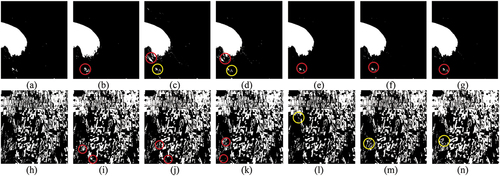
Table 9. Typical feature extraction thresholds and Kappa coefficient statistics.

Region	Sensor	Threshold	Kappa1	Threshold	Kappa 2	Validate the data
Bortala Mongolia NDWI	GF-1 WFV4	0.14	0.9470	0.20	0.9614	Landsat8
	GF-6 WFV	0.14	0.9615	0.20	0.9522	Landsat8
	GF-1 trans WFV	0.14	0.9528	0.20	0.9603	Landsat8
Changji NDVI	GF-1 WFV4	0.42	0.9193	0.46	0.9285	Landsat8
	GF-6 WFV	0.42	0.9222	0.46	0.9074	Landsat8
	GF-1 trans WFV	0.42	0.9204	0.46	0.9291	Landsat8

During the feature extraction process, combining the index method with threshold adjustment effectively enhances visualization and ensures good consistency with validation data (as shown in Figure 7). It is noteworthy that the data transformed from GF-6 to GF-1 trans are closer to the original GF-1 data in vegetation and water body extraction, rather than GF-6. Even when the threshold is set to 0.42 or 0.46, the visual differences between GF-1 and GF-6 in surface cover feature extraction are not significant.

Table 9 data indicate minimal variation in Kappa coefficients within the optimal threshold range, revealing subtle differences in extraction accuracy among GF-1 WFV4, GF-1 trans WFV and GF-6 WFV, but overall proximity. At lower thresholds, the accuracy of GF-6 WFV and GF-1 trans WFV surpasses that of GF-1 WFV4; whereas, at higher thresholds, the accuracy of GF-1 WFV4 exceeds that of GF-6 WFV and GF-1 trans WFV, with GF-1 trans WFV particularly approaching the accuracy of GF-1 WFV4.

The comprehensive analysis suggests that, in vegetation and water body information extraction scenarios, the required threshold for GF-6 WFV is generally lower than that for GF-1 WFV4, implying that threshold setting is not directly correlated with overall image reflectance. This phenomenon suggests that different sensors may require threshold optimization based on their own characteristics to achieve optimal extraction efficiency. Furthermore, the comparative study between GF-1 trans WFV and GF-1 WFV4 indicates that an effective conversion from GF-6 to GF-1 is feasible, and the two sensors complement each other in practical applications.

Among the three study areas in this paper, the experimental image of Changji is dominated by vegetation, Bortala Mongolia is covered with water bodies, and the validation images contain water bodies and vegetation distribution. Thus, 60 water body ROIs are selected in each of the Bortala Mongolia and Hohhot areas, and 60 vegetation ROIs are selected in each of the Changji and Hohhot regions to better analyse the relationship between feature extraction and the two sensors. This approach was undertaken to delve into the performance of GF-1, GF-6 and GF-1 trans in recognizing different land cover types.

The results from Figures 8 and 9 reveal distinct reflectance patterns between GF-1 and GF-6 satellites across the study areas of Changji, rich in vegetation, and Bortala Mongolian Autonomous Prefecture, dominated by water bodies. In the vegetation-rich Changji region, GF-1 exhibits a lower reflectance in the blue, green and red visible bands compared to GF-6, while both satellites show similar trends in the near-infrared band. Conversely, in the water-covered region of the Bortala Mongolian Autonomous Prefecture, GF-1 displays higher reflectance in the blue, green and red bands than GF-6, with slightly lower reflectance in the near-infrared band. In the diverse land cover region of Hohhot, the reflectance differences between GF-1 and GF-6 satellites across various bands are notably reduced.

Figure 8. The plot of water bodies ROI in the corresponding bands in Bortala Mongolia and Hohhot versus y=0.

Figure 9. The plot of the vegetation ROI in the corresponding bands in Changji and Hohhot versus.

Comparing GF-1 trans with original GF-1 imagery, in the vegetation-rich Changji area, although GF-1 trans exhibits lower reflectance in the blue, green and red bands compared to GF-1, its reflectance is slightly higher in the near-infrared band, with minimal differences between the two, and their values are distributed near the y = 0 axis. In the water-dominated region of the Bortala Mongolian Autonomous Prefecture, the reflectance values of GF-1 trans and GF-1 fluctuate closely around the y = 0 axis, indicating minimal differences between them. As for the Hohhot region, regardless of water bodies or vegetation, the reflectance values of GF-1 trans are nearly identical to those of GF-1, with differences strictly controlled within ± 0.001.

In summary, although GF-1 and GF-6 exhibit different response characteristics in land cover feature extraction, appropriate transformation methods have significantly aligned the reflectance values of GF-1 trans imagery with those of original GF-1 imagery across various bands. The differences between the two can be considered non-significant within acceptable ranges, thus validating the effectiveness of the employed transformation equation. Consequently, under specific conditions, GF-1 and GF-6 satellite data can be mutually transformed using rational conversion models, facilitating interoperability and complementary applications of the data. These research findings deepen the understanding of performance characteristics of these two remote sensing sensors and provide important technical support and practical guidance for cross-sensor data fusion, land cover classification and related fields.

5. Discussion

In this paper, the sensor data of GF-1 WFV4 and GF-6 WFV are quantitatively analysed in the sample area by using the TOA mean comparison method. The verification results in Hohhot show that the two sensors have good consistency between the corresponding bands, but there are still certain differences, e.g. the signal of GF-1 WFV4 is generally stronger than that of GF-6 WFV, and the performance differs in different bands for different ground objects.

1. Differences in spectral response functions: There are certain differences in the spectral response functions of GF-1 WFV4 and GF-6 WFV sensors, and the spectral coverage is not completely consistent (Figure 10). The difference in spectral curve function agrees with the ME results obtained by comparing the Bortala Mongolia image pair and the Changji image pair based on the mean TOA in the sample area, and the differences are obvious for different land feature types in different areas. According to the results of the TOA mean comparison method in the sample area, the ME of Bortala Mongolia image pairs are sorted in descending order as green > blue > red > NIR, and the ME of Changji image pairs is green > NIR > red > blue; the RSME of Bortala Mongolia image pairs are sorted in descending order as green > blue > NIR > red, the RSME of Changji image pairs is NIR > blue > red > green, and the RSME of Hohhot image pairs is red > NIR > green > blue. From the conversion equation verification, it can be seen that MAPE and RMSE vary more at the green band and less at other bands. In general, the spectra of the GF-1 WFV4 and GF-6 WFV sensors differ greatly in the green band, the simulated decline is the largest, and the difference in this spectral response function will lead to differences in the reflected signals of the features received by the two sensors in the green band.

   Figure 10. Relative Spectral Response of GF-1 WFV4 and GF-6 WFV.

   

2. Differences in radiometric resolution (Chander, Meyer and Helder 2004). The 12-bit radiometric resolution of GF-1 WFV4 is higher than the 10-bit radiometric resolution of GF-6 WFV, so GF-1 WFV4 has a higher ability to perceive small changes in the emitted or reflected energy of objects than GF-6 WFV. Meanwhile, as can be seen from Table 2, the dynamic range of DN values is subject to the radiometric resolution, and in the two experimental areas, the dynamic range of the four bands of GF-1 WFV4 is larger than that of GF-6 WFV.

3. Difference of satellite side view: The difference of satellite side view between GF-1 WFV4 and GF-6 WFV for the Bortala Mongolia image pair is large, while that for the Changji and Hohhot image pairs is small, and the influence of satellite side view should be considered when performing image correction.

4. Noise-Level Differences: The signal-to-noise ratio (SNR) between GF-1 WFV4 and GF-6 WFV may vary, which can impact the final image quality and the accuracy of land cover recognition. Generally, a higher radiometric resolution is associated with lower noise levels, allowing GF-1 WFV4 to provide more detailed and clearer information about land cover to a certain extent.

5. Data Complementarity. In the context of long-term remote sensing image research, given the unique advantages and similar spectral response characteristics exhibited by the GF-1 and GF-6 satellites under various ground object conditions, it is recommended to integrate the data resources of GF-1 and GF-6. The rationale behind this integration is to compensate for any data gaps or insufficiencies within a given time period using the data from the alternate satellite, thereby ensuring the completeness and coherence of the time-series data. Such a method of data complementarity can maximize the synergistic effects of both satellites, significantly enhancing the accuracy and reliability of the analysis outcomes.

6. Conclusion

In this paper, the corresponding bands of GF-1 WFV4 and GF-6 WFV sensors are compared based on the TOA mean comparison method by using the same-day transit image pairs in Bortala Mongolia and Changji areas. The results indicate that the corresponding band data of the two sensors have a strong correlation (R² is greater than 0.90). Meanwhile, RMSE of the three pairs of images for other corresponding bands is less than 0.05, so there is a strong correlation and complementarity between the two data of GF-1 WFV4 and GF-6 WFV. The interactive comparative experiment shows that the signals of the two sensors differ in different areas. The amount of feature information and the signal strength of GF-1 WFV4 are generally greater than those of GF-6 WFV in the Bortala Mongolia area, with an overall MAPE mean difference of 8.37%; the amount of feature information and the signal strength obtained by GF-1 WFV4 are generally smaller than those of GF-6 WFV in the Changji area, with an overall MAPE mean difference of 8.23%. The results indicate that the difference in the data between the GF-1 WFV4 and GF-6 WFV is caused by the difference in the spectral response function and radiometric resolution of the two sensors. Although there are differences between the two sensors of GF-1 WFV4 and GF-6 WFV, the data of the two sensors can be converted and verified by the linear regression equation obtained in this paper. Besides, the data converted by the linear regression equation between the two sensors can greatly reduce the gap between the spectral data of the two sensors, and the data coincidence is significantly improved. Moreover, the experiment using the exponential method to extract the same ground feature shows that the selection of the threshold does not depend on the overall reflectivity. In conclusion, when extracting different ground feature types (water bodies or vegetation), the feature extraction threshold of GF-6 WFV is smaller than that of GF-1 WFV4, and the extraction accuracy is comparable. Through the transformation equation, converting GF-6 imagery to GF-1 imagery and conducting comparative analysis reveals that the transformed GF-1 imagery exhibits minimal differences in extraction compared to the original GF-1 imagery. This implies that GF-6 and GF-1 can be mutually transformed under specific conditions using appropriate transformation equations, thereby compensating for the limitations of a single data source. However, due to the influence of both sensors’ transit time and cloud amount, the features in the three pairs of images selected in this paper are relatively single, the obtained conclusions inevitably have limitations, and further comparative studies of sensor data in a larger spatial range are necessary.

Author contribution

YGG and MZF designed the experiments and wrote the manuscript; YGG reviewed the manuscript; MZF ran the experiments; YGG performed the verification analysis; HQX contributed to the design of the experiments. All authors read and approved the final manuscript.

Acknowledgements

The authors would like to thank China Resources Satellite Application Center (www.cresda.com/CN/) for the data support.

Disclosure statement

No potential conflict of interest was reported by the author(s).

Data availability statement

The data that support the findings of this study are available from the corresponding author, upon reasonable request.

Additional information

Funding

The work was supported by the Nature Science Foundation of Fujian Province, China [2023J01064].

References

- Camps-Valls, G., L. Gomez-Chova, J. Munoz-Mari, J. L. Rojo-Alvarez, and M. Martinez-Ramon. 2008. “Kernel-Based Framework for Multitemporal and Multisource Remote Sensing Data Classification and Change Detection.” IEEI Transactions on Geoscience and Remote Sensing 46 (6): 1822–1835. https://doi.org/10.1109/TGRS.2008.916201.
- Chander, G., M. J. Coan, and P. L. Scaramuzza. 2008. “Evaluation and Comparison of the IRS-P6 and the Landsat Sensors.” IEEI Transactions on Geoscience and Remote Sensing 46 (1): 209–221. https://doi.org/10.1109/TGRS.2007.907426.
- Chander, G., B. L. Markham, and D. L. Helder. 2009. “Summary of Current Radiometric Calibration Coefficients for Lan-Dsat MSS, TM, ETM+, and EO-1 ALI Sensors.” Remote Sensing of Environment 113 (5): 893–903. https://doi.org/10.1016/j.rse.2009.01.007.
- Chander, G., D. J. Meyer, and D. L. Helder. 2004. “Cross Calibration of the Landsat-7 ETM+ and EO-1 ALI Sensor.” IEEI Transactions on Geoscience and Remote Sensing 42 (12): 2821–2831. https://doi.org/10.1109/TGRS.2004.836387.
- Chen, X., V. Lee, and D. Don. 2005. “A Simple and Effective Radiometric Correction Method to Improve Landscape Change Detection Across Sensors and Across Time.” Remote Sensing of Environment 98 (1): 63–79. https://doi.org/10.1016/j.rse.2005.05.021.
- Chen, Y., K. Sun, D. Li, T. Bai, and C. Huang. 2017. “Radiometric Cross-Calibration of GF-4 PMS Sensor Based on Assimilation of Landsat-8 OLI Images.” Remote Sensing 9 (8): 811. https://doi.org/10.3390/rs9080811.
- Du, T. 2015. “The Comparison Among Fusion Algorithms of Landsat8 OLI Remote-Sensing Imagery and the Analysis on Adaptability of the Classification of Land Use.” Master’s thesis, Northwest University.
- Gao, Y. 2013. “Study on the Application of Multi-Source and Multi-Scale Images in the Urban Remote Sensing.” Dissertation, Fuzhou University.
- Goward, S. N., P. E. Davis, D. Fleming, L. Miller, and J. R. Townshend. 2003. “Empirical Comparison of Landsat 7 and IKONOS Multispectral Measurements for Selected Earth Observation System (EOS) Validation Sites.” Remote Sensing of Environment 88 (1–2): 80–99. https://doi.org/10.1016/j.rse.2003.07.009.
- Jiang, Q., and H. Xu. 2018. “Cross-Comparison Between GF-1 PMS2 and GF-2 PMS2 Sensor Data.” Remote Sensing Technology and Application 33 (6): 1084–1094. https://doi.org/10.11873/j.issn.1004-0323.2018.6.1084.
- Li, P., L. Jiang, and Z. Feng. 2014. “Cross-Comparison of Vegetation Indices Derived from Landsat-7 Enhanced Them-Atic Mapper Plus (ETM+) and Landsat-8 Operational Land Imager (OLI) Sensors.” Remote Sensing 6 (1): 310–329. https://doi.org/10.3390/rs6010310.
- Mishra, N., M. Haque, L. Leigh, D. Aaron, D. Helder, and B. Markham. 2014. “Radiometric Cross Calibration of Landsat 8 Operational Land Imager (OLI) and Landsat 7 Enhanced Thematic Mapper Plus (ETM+.” Remote Sensing 6 (12): 12619–12638. https://doi.org/10.3390/rs61212619.
- Padró, J., X. Pons, D. Aragonés, R. Díaz-Delgado, D. García, J. Bustamante, L. Pesquer, et al. 2017. “Radiometric Correction of Simultaneously Acquired Landsat-7/Landsat-8 and Sentinel-2A Imagery Using Pseudoinvariant Areas (PIA): Contributing to the Landsat Time Series Legacy.” Remote Sensing 9 (12): 1319. https://doi.org/10.3390/rs9121319.
- Roy, D. P., V. Kovalskyy, H. K. Zhang, E. F. Vermote, L. Yan, S. S. Kumar, and A. Egorov. 2016. “Characterization of Landsat-7 to Landsat-8 Reflective Wavelength and Normalized Difference Vegetation Index Continuity.” Remote Sensing of Environment 185:57–70. https://doi.org/10.1016/j.rse.2015.12.024.
- Shan, W., X. Jin, X. Meng, X. Yang, Z. Xu, Z. Gu, Y. Zhou, and A. David. 2019. “Dynamical Monitoring of Ecological Environment Quality of Land Consolidation Based on Multi-Source Remote Sensing Data.” Transactions of the Chinese Society of Agricultural Engineering 35 (1): 234–242. https://doi.org/10.11975/j.issn.1002-6819.2019.01.029.
- She, X., L. Zhang, Y. Cen, T. Wu, C. Huang, and M. Baig. 2015. “Comparison of the Continuity of Vegetation Indices Derived from Landsat 8 OLI and Landsat 7 ETM+ Data Among Different Vegetation Types.” Remote Sensing 7 (10): 13485–13506. https://doi.org/10.3390/rs71013485.
- Song, X., W. Huang, M. C. Hansen, and P. Potapov. 2021. “An Evaluation of Landsat, Sentinel-2, Sentinel-1 and MODIS Data for Crop Type Mapping.” Science of Remote Sensing 3:100018. https://doi.org/10.1016/j.srs.2021.100018.
- Sun, T., S. Feng, and Y. Xu. 2012. “Study on Relationship Between IRS-P6 LISS-3 and Landsat-5 TM Remote Sensing Images.” Remote Sensing Technology and Application 27 (6): 887–895.
- Teillet, P. M., J. L. Barker, B. L. Markham, R. R. Irish, G. Fedosejevs, and J. C. Storey. 2001. “Radiometric Cross-Calibration of the Landsat-7 ETM+ and Landsat-5 TM Sensors Based on Tandem Data Sets.” Remote Sensing of Environment 78 (1): 39–54. https://doi.org/10.1016/S0034-4257(01)00248-6.
- Vogelmann, J. E., D. Helder, R. Morfitt, M. J. Choate, J. W. Merchant, and H. Bulley. 2001. “Effects of Landsat 5 Thematic Mapper and Landsat 7 Enhanced Thematic Mapper Plus Radiometric and Geometric Calibrations and Corre-Ctions on Landscape Characterization.” Remote Sensing of Environment 78 (1): 55–70. https://doi.org/10.1016/S0034-4257(01)00249-8.
- Wang, L., R. Yang, Q. Tian, Y. Yang, Y. Zhou, Y. Sun, and X. Mi. 2015. “Comparative Analysis of GF-1 WFV, ZY-3 MUX, and HJ-1 CCD Sensor Data for Grassland Monitoring Applications.” Remote Sensing 7 (2): 2089–2108. https://doi.org/10.3390/rs70202089.
- Wu, X., H. Xu, and Q. Jiang. 2020. “Interaction of Multispectral Data from GF-1, GF-2 and Landsat-8 Satellites.” Geomatics and Information Science of Wuhan University 45 (1): 150–158.
- Xu, G., and H. Xu. 2021. “Cross-Comparison of Sentinel-2A MSI and Landsat 8 OLI Multispectral Information.” Remote Sensing Technology and Application 36 (1): 165–175. https://doi.org/10.11873/j.issn.1004-0323.2021.1.0165.
- Xu, H., Z. Liu, and Y. Guo. 2016. “Comparison of NDVI Data Between GF-1 PMS1 and ZY-3 MUX Sensors.” Transactions of the Chinese Society of Agricultural Engineering 32 (8): 148–154. https://doi.org/10.11975/j.issn.1002-6819.2016.08.021.
- Xu, H., F. Sun, and G. Xu. 2021. “Cross Comparison of Radiance Data Between Hyperspectral AHSI and Multispectra-L VIMI Sensors of Gaofen-5 Satellite.” Geomatics and Information Science of Wuhan University 46 (7): 1032–1043. https://doi.org/10.13203/j.whugis20200586.
- Xu, H. X., T. Zhang, and C. Li. 2011. “Cross Comparison of Thermal Infrared Data Between ASTER and Landsat ETM~+ Sensors.” Geomatics and Information Science of Wuhan University 36 (8): 936–940. https://doi.org/10.13203/j.whugis2011.08.017.
- Xu, Y., H. Zhang, Z. Chen, and H. Jing. 2018. “A Case Study on Pixel-By-Pixel Radiometric Normalization Between Sentinel-2A and Landsat-8 OLI.” Paper presented at the 2018 Progress in Electromagnetics Research Symposium (PIERS-Toyama), 1188–1193. Toyama, Japan.
- Ye, X., H. Ren, Y. Liang, J. Zhu, J. Guo, J. Nie, H. Zeng, Y. Zhao, and Y. Qian. 2021. “Cross-Calibration of Chinese Gaofen-5 Thermal Infrared Images and Its Improvement on Land Surface Temperature Retrieval.” International Journal of Applied Earth Observation and Geoinformation 101:102357. https://doi.org/10.1016/j.jag.2021.102357.
- Zhang, Y., Z. Feng, and D. Shi. 2007. “The Influence of Satellite Observation Direction on Remote Sensing Image.” Journal of Remote Sensing 11 (4): 433–438.
- Zhang, Y., L. Yu, M. Sun, and X. Zhu. 2017. “A Mixed Radiometric Normalization Method for Mosaicking of High-Resolution Satellite Imagery.” IEEI Transactions on Geoscience and Remote Sensing 55 (5): 2972–2984. https://doi.org/10.1109/TGRS.2017.2657582.
- Zhao, L., R. Zhao, Y. Liu, and X. Zhu. 2020. “The Differences Between Extracting Vegetation Information from GF1-WFV and Landsat8-OLI.” Acta Ecologica Sinica 40 (10): 3495–3506. https://doi.org/10.5846/stxb201903040405.
- Zhong, H., J. Bian, and A. Li. 2018. “Radiometric Consistency Between Landsat 8 OLI and Sentinel-2 MSI Imagery in Mountainous Terrain.” Remote Sensing Technology and Application 33 (3): 428–438. https://doi.org/10.11873/j.issn.1004-0323.2018.3.0428.