The function of open-field farming – managing time, work and space

ABSTRACT

Open fields were a dominant agricultural feature in Central, Western and Northern Europe for nearly a millennium. The spatial organisation of villages and the degree of communal management of common resources varied, but the basic characteristics and common features of the open-field system were that individual holdings were fragmented into several small unfenced plots and intermingled in one or more fields. Research on the subject is extensive, and several explanations for its cause(s) have been presented; however, the answer regarding the question of its rationale and persistence over time is still up for debate.

The overarching aim of this article is to present new findings concerning open-field farming from a functional and practical perspective. What were the farming practices and how was the spatial organisation in open fields integrated in those practices? This article shows that the common practice in Skaraborg County, Sweden, was diversification by using different crops. In the village of Kleva, the preparation of plots and the planting of different crops was carried out in a sequence. Sources indicate that the scattered plots in open fields were integrated into that sequence and that certain plots were designated for certain crops to be sown at a certain moment in time. In the village of Kleva, open fields were used to cater to precision farming as a way to manage time, work and space.

Keywords:

• Open field
• historical geography
• agrarian history
• farming practice
• time geography

INTRODUCTION

The aim of this paper is to study the function of the open-field system and the agricultural practices associated with open fields before the agricultural revolution associated with land reorganisation in the seventeenth and eighteenth centuries led to the consolidation of holdings and the abandonment of the open-field system. To study the function of open fields, this article will analyse farming practices and transportation costs on farms in relation to time, work and space. What was the functional logic behind the complex spatial arrangements in open-field villages and how were fragmented holdings integrated into the open-field farming practice?

The open-field system was the dominant agricultural system in Northern Europe for nearly a millennium and is still in use in some parts of Europe (Renes 2010, pp. 37, 65). The term ‘common fields’ is sometimes used as a synonym for open fields, but there is an important distinction to be made between the two terms, as Mark Bailey (2010) and Stefano Fenoaltea (1988) note. While the term ‘open fields’ refers to the physical division of land in scattered and intermingled individual holdings in unfenced strips/ blocks in the arable field, the term ‘common fields’ refers to the system as a whole, i.e., the overarching system that is characterised by common regulations of resources, fallow, cropping, and grazing in one or more open fields (Bailey 2010, p. 156; Fenoaltea 1988, p. 171). Common fields always include one or more open fields, but open fields can also exist without common regulation in common fields. There is a wide range of different local and regional varieties of open and common fields regarding both layout and organisation, but some basic common features define them. How these terms are used in the literature varies. In their conclusions, Dyer, Thoen and Williamson (2018, p. 258) introduce a revised definition and characterisation of open fields in which the term ‘open fields’ encompasses the above-mentioned definitions of both open and common fields. In this article the term ‘open fields’ refers to the physical phenomenon of fragmented holdings in arable fields.

The origin of the open-field system has occupied the historical studies of research communities in geography and economic history throughout the twentieth century. A number of explanatory models of different causes of the establishment of open fields have been presented. Scattering in open fields has been theorised to be the result of 1) egalitarianism/ equal sharing (Maitland 1897; Vinogradoff 1892); 2) piecemeal reclamation; 3) partible inheritance; 4) population pressure (Campbell 1981; Dyer et al. 2018; Thirsk 1964); 5) risk management/ insurance (McCloskey 1972, 1991); 6) institutional arrangements/ common grazing (Dahlman 1980); and 7) collective control and property rights (Smith 2000). These different models have been used both as monocausal explanations and in combination, where one could be more dominant than the other(s) in different regions (Campbell 1981; Dodgshon 1980).

This article agrees with McCloskey that ‘the origin of open fields is less important than their reasons for persisting over many centuries’ (McCloskey 1991, p. 344) and that the purpose of fragmented holdings is of more interest than the time of their establishment. Economical and practical assumptions about historic farming that are brought into the analysis affect the answer to the question of why holdings were scattered. Fenoaltea argues that explanations miss the mark when the causes are viewed ‘not as secondary benefits of a productivity-maximising system, but as the primary benefits of a productivity-sacrificing one’ (1988, p. 215). The functional perspective, i.e., the idea that scattered holdings were an integrated part of the farming practice, tends to be ignored.

Economic and labour efficiency/ inefficiency and rationale stand in the centre of the openfield debate. Why did peasants in large parts of Europe organise farming in villages in common arrangements, with fragmented holdings in a complex spatial organisation? Various explanations have been put forward in research, but there are still questions and uncertainties regarding the functionality of open fields.

Open fields are a spatial phenomenon, and their spatial layout must be analysed in regard to how that spatiality was used and how it was functionally linked to the practice of agricultural production. Agriculture is all about work, time and space; these three variables were functionally linked to the physical structure of the open field. As Howarths puts it (emphasis in the original), ‘The key idea is to link a map of space to a plan for space, where the plan provides functional reasons why a space should be arranged in a particular way in order to fulfil a particular purpose’ (Howarths 2008, p. 92).

To understand open fields, we must determine the purpose of the spatial organisation of holdings that we see in the large-scale maps, how that organisation was utilised in practice and integrated into farming practices, and the potential benefits of the said organisation.

Maps are the result of what a surveyor saw, measured, and depicted at a specific point in time, even though they are a simplification of reality; a map is more than just a colourful depiction. Maps allow for analyses of places and functions on different scales, as well as of the space-time movements of activities within the confines of the surveyed area. Combining maps with information from other sources concerning the same place allows for detailed analyses (and estimates) of agricultural practice in the open-field system. A map sets the space-time possibilities and limitations for the practice of agriculture and delineates the time-geographical prism in which farming activities take place. The practice of agriculture is a continuous rotation and movement of different actions in scattered locations at different moments in time.

This article shows how scattered holdings in open fields were integrated into farming practices and facilitated the management of time, work and space. Furthermore, this study stresses the importance of a functional perspective in analysing and understanding open fields. In the three-field system, work (i.e., preparation and sowing) was spatially and temporally distributed in a sequence in which different crops were sown in specific topographical and soil conditions and thereby at different moments in time, depending on both the difference in the ‘growth period’ between crops and the ‘best time’ for a specific crop. In this way, intermingled holdings were a part of the technological complex of mixed farming and the manual labour through which it was carried out. To analyse the spatial and temporal precision in open-field farming, this article aims to answer the following three questions based on empirical evidence:

1. How were fragmented holdings incorporated into farming practices?

2. What chores were involved in farming and how much time did they require?

3. What were the transportation costs in open fields?

The outline for this article is as follows. The section Time, Work, and Space outlines the methodological and theoretical approaches or framework for the study. In the succeeding section, The Open-Field Village, the studied village, Kleva, and the source materials are presented. In Crops, Acreage, and Spatial Management, spatial and statistical data based on the sources are presented. The section elaborates on the methodological approach to interpret empirical data in order to reconstruct how farming was carried out. In the following section, Cultivation and Transportation — Time Estimations, the empirical data are processed to make time estimations for the different chores and transportations involved in farming practice. The results and analysis of the study are presented in the closing sections, Results and Discussion.

TIME, WORK, AND SPACE

This article focuses on the functionality of open fields with scattered holdings in historical farming and how their spatial organisation was utilised in everyday work practices. To understand farming practised in open-field villages, we need to analyse the actual chores involved in working the arable, the work input and the time that these chores demanded, and the actual transportation costs in relation to the total amount of labour that was spent in the field(s).

The question of why farming was organised in open fields often stresses the contradictions inherent in a spatial organisation with intermingled holdings and common regulations that have been considered tedious and have sacrificed productivity and possibly efficiency (McCloskey 1972, p. 17). The assumption that the transportation costs in open fields must have been very high is an exaggeration; however McCloskey’s conclusion is based on approximations (McCloskey 1975, p. 78). Transportation costs have actually not been empirically tested. To understand the rationale and function of scattering, a microperspective on individual holdings is needed to examine how individual plots were integrated into farming practices.

Research on open fields has not been particularly spatial/ geographical, at least not at the detailed level of individual farms and individual plots. A time-geographical approach can be useful to analyse and understand the everyday activities associated with farming. The timegeographical approach was formulated by the geographer Torsten Hägerstrand (1985; 2009). Time-geography focuses on individuals and ‘. . . how they use their knowledge, objects and tools. And it investigates how they are involved in social relations and perform activities in the physical real-world environment’ (Ellegård 1999, p. 167). The activities involved in farming (on a family basis) are confined in space and time, and the possible activities (work and otherwise) are affected by a number of constraints in the physical and social context.

In time-geographical studies, path, place and time are fundamental. Work involves movement, places and time (spent). Humans cannot physically be in two places at the same time; the ability to carry out one’s activities is limited by constraints and is dependent on decisions made at an earlier time, as well as on social and organisational obligations, structures, location, and access to resources. Within the time-geographical approach, the main constraints are capacity, coupling, authority, and movement (ibid., p. 167). The time-geographical approach is used to study activities performed by individuals on a micro-level and how individuals make use of available resources and fulfil those activities. By ‘tracking’ everyday activities and how time-space implications or configurations affect these activities, an individual’s movements in time and space are mapped. Activities in openfield cultivation are trajectories in time-space and, depending on the type of activity, the duration and the location, they are subject to constraints. This space of activity forms a so-called prism (Lenntorp 2005, pp. 223–4), which means that the time spent on an activity limits the distance of where it is carried out in relation to the home. The most common argument for the inefficiency of open fields is actually essentially a time-geographical argument. Scattering one’s holdings in a number of places means more work (transportation) and more time spent. However, farming could also be defined as one’s ability to navigate climatic and topographical constraints by adapting one’s activities and technologies to the right or most adequate space at just the right moment. The right time to act is thus another important constraint that has to do with knowledge and experience. In agriculture and spatial contexts, this is known as when, how, and where to act.

Using time-geography to study historical geography and the spatial organisation of open fields poses challenges. Time-geography studies behaviour, activities and choices made by the study subject(s) in time and space, and these activities delimit the space in which these activities take place. The temporal and spatial propagation is observed and then analysed. In this article, activities in historical farming are reconstructed to analyse their potential temporality and spatiality. The approach is, in a way, used backwards and aims to decipher how the spatial layout of open fields was used in farming practices. The overall spatial plan is determined through the analysis of detailed maps of villages, but the details of how this plan was used remain the question.

In whatever economic context farming takes place, the basic goal is to produce an output that exceeds the input. The key to a good result is intensification, i.e., the amount of times a certain area is worked/ prepared before sowing (Myrdal 1985, p. 92). A block or strip of land that is ploughed once and then sown will yield less than if the same area is ploughed two or three times, run over with a harrow twice and then possibly compressed. Working the fallow will also increase the output, and the same principle is relevant here: the number of times the fallow is worked, the better the outcome. Myrdal talks about technological complexes, where one or more technological innovations enable, or lead to, new practices. The iron shovel enabled land reclamation, made digging ditches more efficient and made wet soils available for production; additionally, the refinement of the ard plough made it suitable for preparing the fallow, which was a prerequisite for the two-field system (Myrdal 1985, p. 151). The development of tools influences farming practices and subsequently has spatial consequences.

Open fields can, in the same way, be incorporated into a technological complex as a spatial consequence of intensified arable farming, where the increased number of times the arable is worked is balanced by a more or less appropriate size of plots. The spatial organisation of the open-field system is most likely to be found in farming practices; it would be highly unlikely that the fragmentation of holdings did not have a direct correlation to farming practices and manual labour. However, this does not mean that any other secondary effects or causes should be ruled out.

THE OPEN-FIELD VILLAGE

The empirical foundation of this study is primarily two source materials: two maps, one from 1688 and one from 1749, and a description of the village of Kleva in south-western Sweden that was written in the 1770–80s. These sources provide information on the spatial organisation of cadastral farms (tax units) and farming practices in the second half of the eighteenth century. In addition, a cadastre (jordebok) from 1566 and tax registers (mantalslängder) from 1645–1764 have been used to give information on the subdivision of cadastral farms and to trace the village further back in time. The situation in Kleva in the eighteenth century was characterised by a population increase and the subdivision of cadastral farms that would eventually result in reorganisation based on the storskifte land reform of 1792.¹

The village is situated on the eastern side of the table-mountain of Kinnekulle on the eastern shore of Lake Värnen in the county of Skaraborg. The open-field villages in Skaraborg are characterised by the unsystematic distribution of holdings and, with its twenty cadastral farms, Kleva would be considered a large village in the Swedish context and representative for the region.

In 1749, Kleva was surveyed, and a geometrical map was produced (Fig. 1).² This map depicts the arable and meadows (infield) and the distribution of the scattered holdings of the village’s twenty cadastral farms in three arable fields (also including meadows) and two meadow fields. The outlying woods and grazing land are excluded. The meadows are coloured green, while the arable is coloured light brown/ orange and grey; the use of different colours is to show which of the three fields lay fallow (grey) and indicates that a three-field system was practised. The map is meticulously made; the surveyor states in the accompanying text that all landowners were present out in the fields to point out each and every holding. When georeferencing this map against a modern map, the measured areas in 1749 match the areas measured in a geographic information system (GIS).³ The map from 1688, which was the first time the village was surveyed, specifies only the plots (arable and meadows) of one of the village farms (farm no. 6 on the 1749 map); however, the arable of the whole village is delineated, which allows for a comparison of the acreage between the two years. The map of 1688 can thus be used to compare the village total acreage between the two years.

Fig. 1. Village of Kleva surveyed in 1749. Shows the village infield (arable and meadows); the woods and grazing land have been excluded. The map was originally made on two different pages. In the image, these have been merged using Photoshop. The orientation is skewed, with the top of the page actually facing northwest. Surveyor: Sven Leffler. Scale 1:4000. Source: LSA P110-3:2.

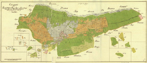
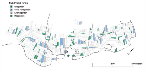
Fig. 2. The map shows the spatial correlation between farm nos 6 and 19 and between nos 7 and 9. Sometime before the records in the cadastre of 1566 the cadastral farms nos 6 and 7 were subdivided, each in two parts. The two farms are noted as half-deserted indicating subdivision. Based on the information in both the 1688 and 1749 maps it is possible to deduce which cadastral farms in the 1749 map that was the result of these subdivisions. This shows that subdivisions in this part of Sweden was done through splitting of each individual plot.

In the 1770–80s, the same village was described in what is called a ‘parish description’ (Sallander 1978).⁴ The parish description has its background in Jakob Faggot’s list of 165 questions, mostly regarding economics, trade and industry, but also history, published at the Swedish Academy of Sciences in 1741 (Gadd 1983, p. 47). Approximately eighty parish descriptions have been preserved from the county of Skaraborg, and they provide detailed information on farming practices; among other things, they describe the field system, technology and tools, the number of draught animals, type of crops, the amount of different crops per farm, preparation and sowing times, the different chores associated with cropping, the available resources, and the quality of pastures and woodlands. The parish description of Kleva was written by the vicar who lived in the village and took part in the open field, which means that he had first-hand knowledge about the farming practices in this specific village. In addition to the parish description of Kleva, this study is based on thirty-five parish descriptions covering 102 parishes/ congregations. The description of Kleva that is the focus of this paper is one of the most detailed.

The map depicts the spatial organisation of the cadastral farms in 1749, but it does not reveal the subdivisions or the actual number of individual farms.⁵ In order to obtain the actual number of farms, tax registers (mantalslängder 1642–1820) have been used. The total number of farms was thirty-nine (1764), but an increase in subdivisions from the early seventeenth century onwards is generally seen. In the tax registers, the cadastral farms are specified with the farm name, the user’s name and the mantal number. A subdivided farm has an additional row under the cadastral name with reference to the additional user of that farm, with the share of each expressed in the mantal. If a cadastral farm with a mantal of 0.5 and 5 ha of arable land was divided into two parts, each of these subdivided farms had 0.25 mantal (the division is not always proportionate) and 2.5 ha of arable land. All farms were spatially and administratively linked to a cadastral farm, but they were independent and equal farming units. However, all farms were not subjected to subdivision; nine of the thirty-nine farms were not subdivided at all, which allows for a retrogressive analysis of these farms’ characteristics (Fig. 4 shows how the farms were divided).

Fig. 3. Digitised and georeferenced map (1749) made in ArcMap 10.4. Only the arable land has been digitised. The black lines represent fences. The steep slope along the western area forms a natural fence, while there is no fence between the neighbouring village (Såntorp) in the south.

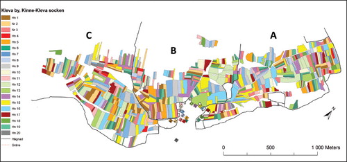
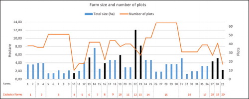
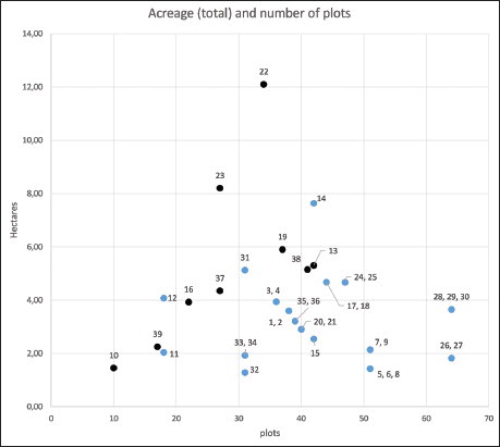
Fig. 4. Farm size and number of plots in Kleva in 1749/1764. Subdivisions are based on the tax register of 1764, and the acreage is taken from the map of 1749. The diagram also show which of the cadastral farms were subdivided and the number of subdivisions. A total of nine of the village farms were not subdivided, and these are marked with black bars (numbers 10, 13, 16, 19, 22, 23, 37, 38 and 39). The right axis and the orange line show the number of plots per farm.

When the open field was laid out, it was not spatially designed for the number of farms, as we shall see later. The cadastre of 1566, in combination with the 1749 map, provides some insights into the subdivisions. In 1566, the village consisted of eighteen cadastral farms, but two of the farms were noted as being half-deserted. Farms noted as being half-deserted is an indication of subdivision; more specifically, it is an indication of hidden subdivision since the practice was illegal by law. Deserted in this context meant that the farms could not pay taxes, not that they were not inhabited (Lindgren 1939, p. 26). What the cadastre shows is that in 1566 the cadastral level was also the farm level, where one family worked the farm, except in the case of the two half-deserted farms; potentially, these two farms were later registered as cadastral farms sometime between 1691 and 1702, according to the tax registers. In total, there were twenty individual farms in 1566 Table 1.

TABLE 1. THE NUMBER OF CADASTRAL FARMS AND SUB-FARMS IN KLEVA IN THE TAX REGISTERS AND CADASTRE. SOURCE: NATIONAL ARCHIVES OF SWEDEN.

The two additional farms identified in the 1566 cadastre can be detected using the two maps of Kleva. In the map from 1749, there are two farms, number 9 and 19, which are mentioned in the map from 1688, and by using the GIS map, it is possible to see how the farms are spatially linked to the cadastral farms from which they were subdivided. Figure 2 shows the distribution of the four holdings and how plots belonging to farm number 19 spatially correlates to the plots belonging to farm number 6, and how they appears side by side throughout the arable fields, and how plots belonging to numbers 7 and 9 appear in the same manner. It should be noted that while the cadastres are a complex source material, they are not comprehensive; thus, additional subdivisions of holdings prior to the 1566 cadastre cannot be excluded.

Using the cadastre and tax registers in combination with the maps and parish descriptions of the spatial configuration, time estimations of the arable work and transportations conducted at the farm level can be analysed. In the spatial analysis below, the acreage generated from the map (1749) has been combined with the number of farms in the tax register of 1764. While the different sources are of different dates, they are quite close in time and have marginal effects on the analysis. The open field in Kleva became increasingly complex over time, but the same sources also offer clues to the village’s earlier history.

As a physical and spatial phenomenon, it is necessary to analyse the actual layout of the openfield system at the farm level in combination with how holdings were actually used over the year to understand their cause and function. Large-scale maps are, by far, the best way to study open fields and are an invaluable source for geographical analysis. The maps are snapshots of a moment in history, of a landscape that is geographically correct, and they also give us information about ownership and land use. By combining the maps with the parish descriptions, it is possible to link and decipher the time-space implications in agricultural practice.

CROPS, ACREAGE, AND SPATIAL MANAGEMENT

From the rectified and georeferenced map of Kleva, various statistics have been generated. In the mid-eighteenth century, the village consisted of thirty-nine farms (in 1764) with a total arable area of 143 ha, based on the survey of 1749. Figure 3 is a digitised (GIS) version of the 1749 map and shows the distribution of the cadastral farm holdings. A comparison between the 1749 map and the 1688 map shows that there was no increase of the arable between these two surveys. Figure 3 shows that Kleva was a nucleated village, and the settlement was grouped in the centre of the village’s arable, with unsystematic open fields. The cadastral farms had a total of 707 plots, but the actual number of arable plots in 1764 was 1,564. The subdivision of the two farms in Fig. 2 indicates that each plot under a cadastral farm was split between the subdivided farms. Subdivisions did not change the number of plots per farm but resulted in a decrease in farm size while the spatial distribution of the cadastral farms was maintained. The average farm’s arable was scattered across thirty-five plots throughout the village’s three fields; however, the village was characterised by diversification in plot size, and the number of plots per farm ranges from ten to sixty-four plots. Farm size is derived from the acreage specified in the map (1749), and the size of the individual subdivided farm is calculated based on the mantal. The size of individual parcels is measured in a digitised map since the map only specifies each farm’s total acreage across the three fields. The sum of the plots in each field on the GIS map corresponds almost exactly with the original map.

Figure 4 shows the arable size of farms in Kleva in 1749 and which of the cadastral farms were subdivided. Eleven cadastral farms were subdivided, while nine farms were not subdivided (specified by black bars in Fig. 4). Twenty-six farms were under 4 ha in size, of which ten were 2 ha or smaller, and thirteen farms were above 4 ha in size. The average total size was 3.7 ha, but the actual sizes varied between 0.77 ha and 12.1 ha, of which two-thirds was used annually.

Generally, the larger cadastral farms were subdivided, although vicarage number 22 and farm number 23 were exceptions. Subdivisions were not even; generally, farms became smaller, but some of the subdivided farms were kept larger than other farms that were subdivided from the same cadastral farm, for example, farm numbers 12, 14 and 31. The line in the diagram (Fig. 4) relates to the right axis and shows the number of plots per farm. The undivided farms are of varying size, but the smaller are of comparable size to the subdivided farms. The important difference is the ratio between farm size and the number of plots, which have functional implications, not the least of which are for costs of transportation.

The trend among the undivided farms is that the number of plots increases with farm size (Fig. 5a). The larger subdivided farms show similar characteristics, while the smaller farms have a certain number of plots (over the village average). The consequences are expected, but the function of subdivision is analysed in the time estimations. The pattern is not as clear regarding average plot size (Fig. 5b), where the general trend is that average plot size decreases with the total number of plots.

Fig. 5a. The relation between farm size and the total number of plots for each farm in Kleva. Statistics generated from the GIS map combined with the tax register information of 1764.

The two cadastral farms that were subdivided into five individual farms each (numbers 3 and 15) both have the highest number of plots, and the majority are smaller than the average size. However, the unsystematic open fields are not only unsystematic in the spatial distribution of plots but also in the size of holdings and the varying plot size. The spatial consequence of subdivision is dependent on the spatial configuration of the cadastral farm that was subdivided.

Development in the seventeenth and eighteenth centuries occurred spatially within the context of the open field. The subdivision of farms led to additional and smaller individual farms with the original spatial configuration intact. Borders in early modern agriculture were stable elements that would not easily change, and this was true both within village boundaries and for individual holdings and plots (Tollin 1999, p. 32).

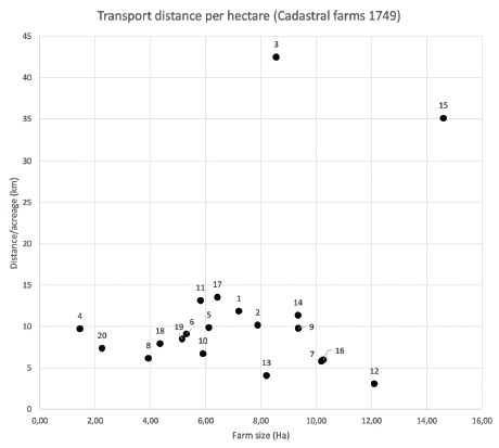
The functional consequence is visualised in Fig. 6a, which displays the required distance per hectare per farm (on average) in relation to farm size (calculations of weighted distance see section Transportation). The undivided farms have a low acreage-distance balance (ten or below), together with some of the larger subdivided farms, while the smaller subdivided farms have a longer distance per hectare. Compared to the distance per hectare at the cadastral level (Fig. 6b), cadastral farm numbers 3 and 15 stand out because of their high number of plots (fifty-one and sixty-four plots, respectively). Their average plot-size is close to or just below the village average, but it is the number of plots that creates the less favourable characteristic. In addition to numbers 3 and 15, other farms (at the cadastral level) show quite similar numbers that are not dependent on farm size. The cadastral level was not the functional level for eleven of the twenty cadastral farms. In 1566 this was most likely the case, even though the farm size was probably smaller. However, their spatial characteristics were most likely the same since the divisions of the holdings were stable and the divisions that we see in 1749 were the same in both arable and meadows. Any expansion of the arable would have taken place in the peripheral areas of the arable fields, not in the centre; therefore, the number of plots and the total distance between the plots and the settlement would also have been lower.

Fig. 5b. The average plot size per farm and total number of plots per farm. Statistics from the GIS map combined with the tax register information of 1764.

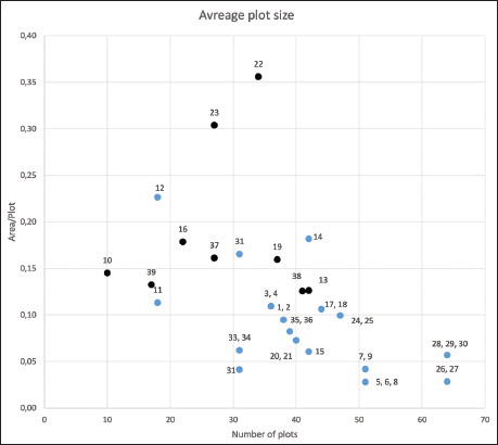
Fig. 6a. The diagram shows the transportation (km) per hectare per farm in relation to farm size.

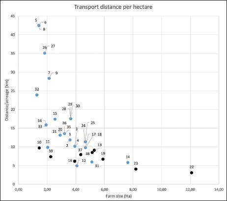
Fig. 6b. Transportation (km) per hectare per cadastral farm. The cadastral farm nos.3 and 15 were divided in 5 farms each. These two farms had the highest number of plots in the village, with 51 and 64, respectively.

The farm-level statistics show both diversity and similarities between the farms and a comparison of the consequences of subdivision between the divided and undivided farms. The question now is, what was preferable and when did spatially dispersed holdings become costly instead of practical? The spatial distribution of plots and the size of individual plots belonging to a farm, whether they are a few large plots or several very small plots, have implications for time consumption, management of working the arable, and time spent on transportation, which are all dependent on the way that plots are clustered. However, these statistics do not take soil quality or topographical conditions into consideration, which are important variables in comparisons between farms.

THE THREE-FIELD SYSTEM

Farming in Kleva was organised in a three-field system, where one of the three fields lay fallow while the other two were in use. Work on the arable and the practice of scattered strips is subordinate to the overarching field system/ fallow system. On the field scale, cultivation in the three-field system was sequenced over a three- year period and based on the combination of spatial and written accounts (parish description) of the practice; thus, it is possible to visualise and identify the labour-intensive periods and their spatial implications. The fence organisation was at the centre of village organisation and was one of the most important institutions in the villages (Myrdal 1996, p. 135). The three-field system of south-western Sweden and the transition from a one-field system (continuous cropping) have been studied in greater depth (Gadd 2018; Kardell 2004; Lindgren 1939).

Of the specified crops in the parish description, autumn crops (wheat and rye) were sown in late August or September, depending on the time of the harvest, while the spring crops (peas, oats, mixed barley, barley, and flax) were sown in April and May (Table 2). In terms of shares, 18 per cent of the total shares were autumn crops, while the spring crops represent 82 per cent of the total shares.

TABLE 2. CROPS USED IN KLEVA. THE PARISH DESCRIPTION SPECIFIES THE AMOUNT OF THE DIFFERENT CROPS AN AVERAGE-SIZED FARM PLANTED. FLAX IS NOT SPECIFIED.

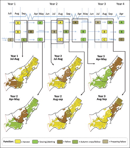
Figure 7 illustrates the fallow rotation and the sequence in which the fields were used for different purposes. The meadow fields visible in Fig. 1 have been excluded, and focus is placed on the arable fields; however, the meadow fields were a part of this rotation and were used for grazing after haymaking (Gadd 2000, p. 114). In the diagram, the timetable of work in the arable specified in the parish description is also visualised spatially using the map to illustrate the rotating functions of the fields. In July of year one, the field that had lain fallow the year before (Field C) was prepared. The plots that would be sown in the autumn were prepared first. The fallow preparations followed the course of ploughing → harrowing → manuring → ploughing. If any weeds grew, then the fallow would be ploughed and harrowed yet again. After the harvest, in Fields A and B, the autumn plots were prepared and sown. Field B would then lie fallow into the second year when Field A and the rest of Field C were sown with spring crops in April and May. This means that Fields A and B were available for pasture on the stubble before taking the livestock inside for the winter. Field C was available for additional grazing after sprouting of the autumn crops (Ehn 1991, pp. 67, 70), after which animals were shut out from the field.

Fig. 7. The diagram illustrates the rotation of fallow, sown, and arable, as well as how the function of the fields changes over a three-year cycle. The maps show the spatial situation at different phases of farming.

The practice of the three-field system meant that 18 per cent of the crops were planted in the autumn of year one in the field that had previously lain fallow, and on average, 37 per cent of the acreage of the fields (A, B, or C) sown in the autumn was designated for autumn crops. Therefore, the main part of cultivation took place in the spring of the following year (year 2), when Field A and the remaining part of Field C were prepared and sown in April/ May. In addition to temporal separation, there was no spatial separation between the autumn and spring crops.

The three-field system has been associated with the introduction of the practice of planting autumn crops, especially autumn rye, in a designated autumn field (Vestbö-Franzén 2005, p. 33). This could have been the case in Kleva at an earlier stage, but, based on the sources, it seems that the use of autumn crops was neither the result of an increased use of autumn rye nor a way to allocate the workload to be carried out at different times. A reasonable conclusion would be that the conditions in Kleva were not suitable for the cultivation of autumn crops and that the use of fallow fields had more to do with limiting the reduction of nutrients, fertilizing, letting the fallow soil rest, and maximising access to pastures. Additional pastures, in addition to the limited waste that the village had access to, are probably more important. Since the village arable and meadows were divided by fences (three arable and two meadow fields), it was possible to manage grazing spatially. The need for pastures must have outweighed the cost of fences, as fence material had to be bought externally (Sallander 1978, p. 70)

CROPS

The number of crops for all the various sizes of farms can be estimated according to data given for a median farm, as shown in Table 2. The parish description makes it clear that these are the crops that farmers used in Kleva; however, for the smaller farms, it is questionable if all of these crops were actually used. The number of crops is specified for an average farm with 1 mantal. Diversification of crops is evident in the majority of villages and hamlets in the parish descriptions (Fig. 8).

Fig. 8. The diagram show the ratio of crops used in parishes based on the thirty-five parish descriptions. The ratio is based on if the crops are mentioned as used crops and not the amount of crops. Each description specifies, with a varying level of detail, the average amount of different crops sown on farm level. The field-systems varies but one-, two- and three-field systems are quite evenly distributed. Descriptions with incomplete information has been excluded. Source: Sundholmska samlingen, Skara stiftsoch landsbibliotek.

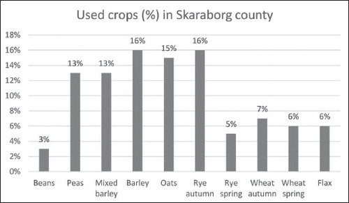
The estimates per average (cadastral) farm in the parish description match the size of the cadastral farms given on the map. The actual average farm size was 3.7 ha, and calculations are made on the actual farm size. The information on crops used and acreage sown per crop has been interpreted as the actual acreage sown and not the number of crops. Different crops were sown with different densities, which in the case of Kleva, would make the sown area, which is based on a differentiated density of seeds per surface unit, approximately 25 per cent smaller and the proportion of autumn crops would increase from 18 to 25 per cent of the total. One barrel of seeds was enough to sow one tunnland of arable or approximately 0.5 ha (Ekstrand 1901, p. 334).

In addition to listing which crops were planted and in what amounts, the parish description also specifies in which sequence the crops were sown and thereby when the spring and autumn preparations started. The parish description specifies the start of spring preparation, according to the Julian calendar, at seven weeks before midsummer, which would be at the end of April in the Gregorian calendar. The date would fluctuate depending on soil conditions, weather and the risk of night frost, and the farmers would wait for the conditions to be right, i.e., the right time to act (Sallander 1978, p. 59).

The first crop to be sown in late April was peas, followed by oats, then mixed barley, and, finally, barley. Sowing in a sequence is described in the majority of the forty parish descriptions used in this study. Information about the localisation of different crops is lacking, but the parish description states that the soil quality in Kleva was highly varied and that while there were some areas with heavy, wet soils, the majority of the areas consisted of sandy, stone-rich soils with a thin overburden.

By combining the spatial information about the size of individual holdings, the number of plots, their distance from the settlement (spatial distribution), and the detailed information about the different chores and their timelines, it is possible to hypothetically estimate the time consumption for working the arable for each farm. One of the basic arguments supporting the obvious shortcomings of fragmented holdings is the transportation cost. What the cost of transportation actually was, and how much time was spent on transportation to and from the plots in the arable in proportion to actual cropping has not been estimated before. This calculation is now possible by combining the study sources. The aim is not to make an exact analysis of the number of people who were actually involved or in what way other farming chores affected work in the arable. The aim is to roughly estimate the time consumption and spatial implications of that practice and workload based on the sources.

CULTIVATION AND TRANSPORTATION — TIME ESTIMATIONS

Making calculations on time consumption in historical farming is precarious, and there are a number of uncertainties and unknowns. There is always a risk that calculations may give a false impression of exact numbers. The ambition herein is to generate a crude but plausible estimate of time consumption for arable farming in order to make a comparison between arable work and transportation costs to thus make a time-geographical analysis of how the fragmented holdings in open fields were integrated in farming practices. Time consumption is estimated for the chores done in the arable (ploughing, harrowing, sowing, compressing, and transportation) for individual farms. The estimates in this article are based on a practical experiment on ploughing by Karlsson (2015), since ploughing is the most time-consuming chore involved in farming, and an agricultural reference book (Sw. betingslära) from 1845.

The agricultural reference book gives information on numerous aspects involved in farming; however, the information is not very detailed, specifically regarding work on the arable. Under the heading plöjning (in English ‘ploughing’), horses were estimated to be able to plough 0.5 ha in one day on moderately hard soils, while oxen could plough 0.375 ha. On heavier clay soils, horses could plough 0.375 ha in one day, while oxen could plough 0.25 ha. Thus oxen required 25 per cent more time to plough the same area than horses. A key issue is that the length of a workday is not specified. Under the heading höbergning (in English ‘haymaking’), it is stated that work from 9 or 10 a.m. in the morning until the evening would make a 0.75 workday. Regarding arable work, the endurance of animals compared to that of farmers is the deciding factor. Myrdal (1981) makes estimations based on nine different reference books from 1690, 1780, 1801, 1850, 1866, 1886, 1921, 1926 and 1932 and estimates the average workday to have been 10 hours, even though the information in the sources varies a great deal. Myrdal specifies that according to books from 1690–1850 and 1926–1932, the average number of workdays needed to plough 0.5 ha was one day; according to the book from 1866, two days were needed, and the books from 1886 and 1921 state that 1.5 days were required (Myrdal 1981, pp. 151–2). According to Myrdal, the ploughing speed did not increase between the seventeenth and nineteenth centuries; on the contrary, it decreased in the nineteenth century due to not only the ploughing of leys and heavier soils but also the increased depth of ploughing from approximately 10 cm in the eighteenth century to 18–20 cm in the nineteenth century (Myrdal 1981, pp. 153–4).

This estimate of one day to plough 0.5 ha is quite consistent with international research, which has found that the medieval farmer could plough an acre a day (Dahlman 1980, p. 27; Langdon 1982, p. 38). A furlong was the length a plough team could pull until it needed to rest, and in a day a plough team could plough the width of 22 yards, which would equal an acre (Bridbury 2008, p. 33).

CHORES

In the case of Kleva, the parish description provides information about the different chores involved, which allows for estimations of cropping as a whole. There are uncertainties, and some generalisations are inevitable. The soils in Kleva are a mix of clays and light, sandy but stone-rich moraine; thus both mouldboard ploughs and ards were used. However, the parish description only describes the practice with the ard, which indicates that the majority of the arable was worked with the ard. Another aspect is the workforce. The number of people who were involved in working the arable on different farms is unknown and therefore not considered.

The chores involved according to the parish description are as follows: ploughing → harrowing → ploughing → sowing → harrowing → compressing. The second ploughing would preferably be performed perpendicular or diagonal to the first furrow. In the parish description, the author notes that the lazy farmer would only plough once (Sallander 1978, p. 62).

ploughing

The time consumption of ploughing is calculated based on the reference book (1845) in combination with the results from Karlsson’s (2015) practical experiments on ploughing. Karlsson performed a series of ploughing tests using horses and a replica of a medieval ard. In addition to measuring the metal wear on the plough, which was the main aim of the experiments, the covered distance for ploughing 1 hectare (recalculated in this article for one tunnland, which is approximately a half-hectare or 4,937 square metres) on a plot of 50 × 100 metres was estimated. The actual speed for ploughing was 4 km per hour; however, including other factors that affected plough speed, such as turning the plough around, stopping for breaks, untangling harnesses, and clearing the ard from soil and weeds, the operational speed was estimated to be 3 km per hour (Karlsson 2015, p. 215).

Gebresenbet et al. (1997) measured different speeds in field experiments with a reversible ardmouldboard plough in Ethiopia. A pair of oxen ploughed at an operational speed of 2.27 km/ hour (in sandy soil) and 2.66 km/hour (in clay), while a pair of cows had an operational speed of 3.02 km/hour in clay; the higher operational speed of cows in this study is explained by the greater body weight of cows compared to oxen (ibid., p. 308). Karlsson ploughed on clay as well but used horses and a different type of ard. Comparing the operational speeds found in the two experiments, the speed of oxen is between 11 and 25 per cent slower than that of the horses in Karlsson’s experiments. In addition to the importance of ploughing at the right or best time, i.e., when the soils are neither too wet nor too dry, speed is a key factor in obtaining a good result. According to Karlsson, a certain amount of speed is necessary for steering and following a straight line, while the equipment becomes unstable and spasmodic when going too fast. The experiments also showed that the shape of the parcel affected the time consumption and speed and that rectangular fields could be ploughed faster due to fewer turns. Thus, a long, narrow strip would be the most time-efficient shape (Karlsson 2015, p. 212).

By Karlsson’s calculations, the travelled distance for ploughing a 50 × 100 metre plot twice would be 35 km plus 8.8 km for turning the plough, or a total of 43.8 km. These calculations are hypothetical, since plots were not perfect rectangles nor were they perfectly flat (ibid., p. 216), but they do give a rough estimate of the distance travelled when ploughing. The ard would cover the width of a metre with three and a half furrows, which means 175 furrows were needed on a 50 metre-wide plot. The extra distance is due to turning the plough around at both ends. In Karlsson’s experiments, different ploughing patterns were tested (ibid., pp. 214–15).

Based on the estimated operational speed of 3 km an hour, it would take 7.3 hours to plough 0.5 ha (Table 3), while ploughing the same area at the speed of 4 km an hour would take 5.5 hours, which would, without considering breaks, mean a difference of approximately 25 per cent in the effective working hours. During a 10-hour day, with an operational speed of 3 km, the effective working hours would be just over 7 hours, but the covered acreage would be somewhat larger than 0.5 ha. Table 3 shows the time consumption for ploughing 0.5 ha twice, based on Karlsson’s estimations. The time consumption for ploughing with oxen is, based on the reference book, calculated as 25 per cent slower than that using horses. Both horses and oxen were used in Kleva, but it is likely that mainly oxen were used; also, when horses were used, it was common to pair them with oxen, which would set the pace.

TABLE 3. THE ESTIMATIONS ARE BASED ON KARLSSON’S (2015) PLOUGHING EXPERIMENTS IN COMBINATION WITH ESTIMATED TIME CONSUMPTIONS FOR DIFFERENT CHORES BASED ON THE AGRICULTURAL REFERENCE BOOK (IN SWEDISH: BETINGSLÄRA) FROM 1845. ACCORDING TO THE REFERENCE BOOK, OXEN WERE 25 PER CENT SLOWER THAN HORSES.

*Distance when turning the plough

**25% slower than horses (Lexikon för landthushållare 1825)

harrowing

The harrow is used for two purposes: breaking up clods to flatten the surface and covering up the broadcast seeds. The chore of crushing the clods is described in the parish description and it states that the arable is run over as many times as needed until the clods are broken to pieces and the surface is smooth (Sallander 1978, p. 61). The reference book (1845) states that harrowing could cover twice the area compared to ploughing. The reference book is quite unspecific in the case of harrowing, and the interpretation is that the specified time consumption is for a specific area harrowed to satisfaction, i.e., when it would be considered done. The second harrowing is supposed to cover the broadcast crops and is assumed to be done by covering the sown plot once at an assumed speed of 5 km an hour. The estimated speed of both harrowing times was set at 5 km per hour. A preferred walking speed for humans is, on average, 5.4 km per hour (for men between age 20 and 50) (Samson et al. 2001, p. 19), and an average brisk walking speed is 8 km per hour (for age 20–70) (Bohannon 1997, p. 17). A speed of 5 km per hour when harrowing is assumed but probable, since the sources say that it is twice as fast as ploughing.

sowing

The number of different crops that could be sown in one day is specified in the reference book under the heading såning: 6 barrels (in Swedish. tunnor) of wheat or peas, 7 barrels of rye, 8 barrels of barley and 12 barrels of oats per day. The reason for the different amounts is the density, specifically the number of seeds per surface unit, which is also specified. In the same book, it states that for one sown barrel of rye (0.5 ha), 0.37 ha of wheat, 0.5 ha of peas, 0.62 ha of barley, and 0.25 ha of oats were also sown. Based on an average of all crops combined, 3.3 ha could be sown in a day, and sowing 0.5 ha would require 0.15 days.

arable work

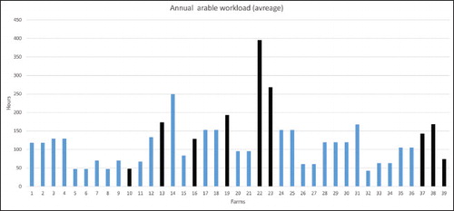
On the basis of the estimated time consumption for the involved chores, the time required for each individual farm has been calculated (see Fig. 9). The diagram shows the average annual workload using oxen as the draught animal. To completely prepare and sow 0.5 ha would require 20.8 hours using horses or 24.5 hours using oxen as draught animals, based on the estimations above. In total, 18 per cent of the arable would have been worked in the autumn, which means that 37 per cent of the autumn field would have been sown in September/ October. The remaining plots in the autumn field were prepared in the following spring, together with the second field. The average-sized farm had an acreage of 3.7 ha and an annual average size of 2.5 ha and would thus require 121 hours of work to prepare and sow the arable, which is the equivalent of 12.1 workdays, excluding time spent on transportation. The subdivided farms had an average workload of 105 hours (10.5 workdays) compared to the undivided (cadastral) farms, which had an average of 168 hours (16.8 workdays). Farm numbers 10 and 39 both deviate from the other undivided farms in their spatial characteristics, size and number of plots. Sixteen farms require less than 100 work hours, and the average workload for these farms is 64 work hours for an average size (annual) of 1.3 hectares. These farms would most likely not have been selfsufficient in grain production and would probably rely on additional means of income. The parish description mentions that farmers were collecting lime stones from the fallow for lime burning and production in the village nursery-garden (collectively owned and used by the village) at the local market (Sallander 1978, p. 72).

Fig. 9. The average annual arable workload per farm. Black bars indicate undivided farms.

To obtain a more complete picture of the time spent and the consequences of scattered holdings, the transportation costs must be included. Calculating distances requires further consideration concerning the actual distances and the number of times that farmers travelled to and from the plots using a carriage.

transportation

The Euclidean distance was generated in GIS, which was not the actual distance that farmers needed to transport their equipment to and from their plots. Walking over another farmer’s plot was unacceptable unless it lay fallow. Comparing the actual distances between the farms and plots in GIS to the Euclidean distances (as the crow flies) shows that the actual distance was longer by a factor of 1.3 when following roads and not crossing any of the other farms’ plots, which is the so-called Manhattan distance. This is consistent with specific research on the subject, which promotes a difference between 1.2–1.4 (Gonçalves et al. 2014, p. 880). The second transportation calculation is based on the practice specified in the parish description.

The practice of sowing the different crops in a sequence means that all chores were completed for each crop in that sequence and that a number of plots (depending on the amount sown per crop) were worked at the same time. The argument is that with many small plots, more than one could be ploughed on the same day, and consequently, transportation would be between the plots, not back and forth to the farmstead for each plot. The key issue is the number of times that farmers had to go back and forth to their plots. Unfortunately, the parish description does not give any specific information about this, but there are some clues. Based on the different chores, the number of times should be six times, which is unlikely considering the fact that the different crops were sown in a sequence and that each chore was not carried out over all of the arable at once but rather for one crop at a time and one cluster of plots at a time. Thus, the estimates for transportation are based on farmers going to and from the plots four times.

To estimate the transportation cost for a number of plots that together would make up 0.5 ha (approximately 2–2.5 workdays) and that would be in spatial proximity to each other, distances have been measured in GIS, including that from the farm to the first plot, then the distance between the plots, and finally the distance from the last plot back to the farm. How this was actually carried out depended on the amount of the different crops. This is a hypothetical calculation of how labour was spatially distributed; however, even though the parish description does not give any specifics about the actual spatial division, it is clear about the sequence, which, given the small size of plots, would undoubtedly mean that more than one plot would be worked at a time.

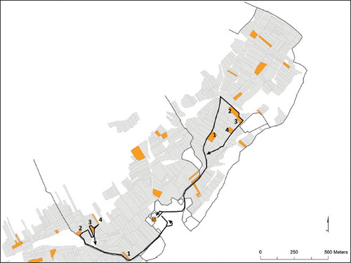
Two examples of the transportation between to clusters of plots are illustrated in Fig. 9. All clusters of plots belonging to farm number 19 (undivided) were measured. In total, the distance travelled is reduced by 54 per cent in Field A, by 31 per cent in Field B and by 40 per cent in Field C. The reduction in transportation in the two fields was used to calculate the time spent on transportation for all the farms. However, the reduction in travelled distance should vary between farms depending on the spatial distribution of their plots; thus, the calculation is approximate for the other farms. Transportation was calculated based on a travelling speed of 3 km per hour. The time spent on transportation was calculated as follows: the Euclidian distance from the settlement to each plot was multiplied by 2 to obtain the total distance, which was then multiplied by a factor of 1.3 to generate a weighted distance, i.e., the Manhattan distance. The weighted distance was then multiplied by the reduction in the travelled distance between the two fields and then finally multiplied by four to compensate for the number of times the farmers had to go back and forth to each cluster Fig. 10.

Fig. 10. The map illustrates how more than one plot was used, and the hypothetical routes have been measured in GIS. The routes follow the roads illustrated on the map (1749) and do not cross any of neighbours’ plots. Measurements have been completed for all of the plots belonging to farm no. 19.

RESULTS AND CONCLUSIONS

By combining sources such as the 1749 map and the parish description, this study shows how farming practices were carried out in Kleva and how those practices were integrated in the spatial layout of the open field(s). Farming in Kleva was diversified by using different crops but also by spatial and temporal diversification. Preparation of the arable involved six chores: ploughing, harrowing, ploughing, sowing, harrowing, and compression, in order to complete the sowing. The chores and location of work were integrated into the sequence of crops, and chores were not carried out one chore at a time within a single plot but for a number of plots and for one crop at a time. Each crop was completed before the next crop was sown. The autumn crops (wheat and rye) were sown in August or September depending on when the harvest was finished. Spring crops (peas, oats, mixed barley, barley, and flax) were sown in late April of the following year. The date would fluctuate depending on soil conditions, weather and the risk of night frost, and farmers would wait for the conditions to be right, i.e., the right time to act.

In terms of shares, 18 per cent of the total crops were autumn crops, while the spring crops represented 82 per cent of the total. In actual land use, approximately 37 per cent of the acreage in the autumn field (A, B or C) was designated for autumn crops. The main part of cultivation took place in the spring of the following year, when the unused field was sown with spring crops and the remaining 63 per cent of the autumn field was also prepared and sown. Aside from the temporal separation of spring and autumn crops, there was no spatial separation between them, and spring and autumn crops were sown in the same field.

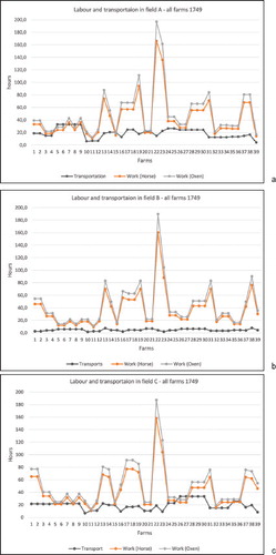
The estimated time required to complete all (six) chores involved to completely prepare and sow 0.5 ha would be 20.8 hours using horses or 24.5 hours using oxen as the draught animals. The use of oxen for ploughing would require approximately 25 per cent more time than that using horses. The average workday is estimated to be 10 hours, with an efficient work time of 7 hours. The time needed for seeding and harrowing was less than that needed for than ploughing. In comparison, ploughing demanded approximately 73 per cent of the total time compared to 27 per cent for harrowing and sowing. Figures 11a, 11b and 11c show the total workload per farm in the three fields (both using oxen and horses).

The tax register of 1764 shows that farms had been subdivided, that the total number of farms was thirty-nine, and that eleven cadastral farms had been subdivided while nine farms remained undivided. Generally, the larger farms were subdivided, but this did not apply to all large farms, and the outcome of subdivision and the number of subdivisions per farm varied (see Fig. 4).

Regarding farm size, sixteen out of thirty-nine farms had an annual acreage of 1.9 ha or less, twenty farms had an arable size of between 2 and 4 ha, and three farms had an acreage of 5 ha or more. Based on the time estimations for arable work, the average workload per farm in Kleva was 121 hours or 12.1 workdays (using oxen), distributed between autumn crops and spring crops. The average total farm size was 3.7 ha, with an average annual size of 2.5 ha.

The workload for the subdivided farms was on average 105 hours, while the average for the undivided farms was 168 hours. However, the small farms, which were unlikely to be self-sufficient, distort the average estimates. Disregarding the sixteen small farms (fourteen subdivided and two undivided), the average workload was 138 hours for subdivided farms and 223 hours for undivided farms, with a combined average of 160 work hours.

Transportation times are estimated based on the plots being worked in clusters, which reduces the amount of transportation since a farmer would not go back and forth to each plot. Figures 11a, 11b and 11c also show the required transportation for each farm in relation to work in the arable. In Fields A and C, the transportation varied between farms between approximately 5 and 45 work hours. In Field B, the transportation was less prominent and stretched between 5 and 21 work hours. For the entire village, 26 per cent of the total workload was spent on transportation. For arable work, the village average hides the variations between the small farms and the larger, self-sufficient subdivided and undivided farms. The transportation share of the total workload was 14 per cent for the undivided farms (over 2 ha) and 22 per cent for the subdivided farms (over 2 ha). For the small farms, i.e., under 2 ha (both subdivided and undivided), the share of the total transportation output was 50 per cent. Figures 12a–c show that farms 5–9, 26–30, and 32 in either two or three fields have a negative balance between transportation and arable work.

Fig. 11a. 11b, 11c. The diagrams show the time spent working the arable and the time spent on transportation in all fields for each farm. Transportation (blue) is defined as the time spent following the measured route back and forth from the farmstead to a cluster (one–four plots) of plots that would constitute an area designated for a certain crop. The results have been multiplied by 4 since all of the different chores would not be completed on one occasion. Orange represents the estimated work using horses, while grey c represents that for using oxen.

The results of the time estimations have been performed for three different categories: farms under 2 ha of annual arable, subdivided farms with more than 2 ha of arable and undivided farms over 2 ha of arable. This is because the aim is to discuss the function of open fields and, over the course of the existence of open fields, the system has not been characterised by subdivision; this is not to say that subdivisions did not occur before the sixteenth century, but it was not to the extent that we see in Kleva in 1764. To understand the practice and its spatial integration in fragmented holdings, the farms that have been unchanged (in addition to increasing the arable) and their spatial configurations are more or less intact.

The main reason that farms under 2 ha (fourteen subdivided and two undivided farms) spent on average 50 per cent of the total transportation workload is because the division of the cadastral holdings was stable and was not subject to any major changes over time. The effect of this spatial continuity of holdings in open fields was that the subdivided farms maintained the spatial configuration of the original cadastral farm but with a significant reduction in farm size. All plots were split so that each farm had a share in each plot but these plots were within each cadastral plot. The result was high transportation cost in relation to work in the arable.

The difference between subdivided and undivided farms (over 2 ha) had the same reason, and the spatial distribution became costly as the farm size decreased. The average size of the subdivided farms was 2.8 ha, while the undivided farms had an average of 4.3 ha. In conclusion, transportation costs were low, with only 14 per cent of the total workload for the undivided farms considered as low. The share of transportations for the subdivided farms was slightly higher at 22 per cent. The subdivisions of the cadastral farms were performed differently, with some farms being kept at a larger size.

The overall workload per farm varied in the same manner as that for transportation. The required arable work might seem low, but farms were relatively small. Subdivided farm number 14 had an annual acreage of 5 ha, which in total would require just under 300 hours or 30 workdays to cultivate all crops for both spring and autumn. This is, however, only an estimate, and the actual time required is impossible to ascertain. It is possible that it would have taken more time, but also less since not every farmer carried out all chores, as the parish description stated that the lazy farmer would not plough a second time (see above and Sallander 1978, p. 62). What is certain is that the sizes of the farms are correct, that these farms worked their lands and that the window of opportunity was the same as it is today. Farmers in Kleva had to act within the available timespan to obtain the best possible outcome.

To analyse the function of open fields in a context in which the basic spatial configuration and practical principles of scattered holdings no longer apply can be misleading. The changes of the holdings through subdivisions changed the prerequisite for open-field farming. Official cadastres and land surveys were preservative in their registration of the holdings and tax units, and the cadastral level (farm level) from the early sixteenth century remained the level of registration over 200 years later. This consistency offers the possibility to study farms, settlements and open fields at an earlier stage using younger sources and a retrogressive approach. In Kleva in 1764, nine farms that were not subjected to subdivision offer valuable clues to the village’s earlier history. The spatial layout of the open field(s) in Kleva is visible on the 1749 map: even though the acreage of the arable land was smaller, many of the arable plots in 1749 were earlierstage meadow plots, and some holdings had been divided (see Fig. 2). There was no expansion of the arable in Kleva between 1688 and 1749, based on comparisons in GIS of the two maps, but any potential increase between 1566 and 1688 is difficult if not impossible to assess. However, the function and integration of open fields into farming practices is possible. The expansion of the arable was generally performed by converting meadow plots to arable, which means that the expansion of the arable would take place in the peripheral areas of the three fields in relation to the settlement. With an expansion of the arable in peripheral plots farther away from the settlement, the transportation costs would have increased in relation to that expansion. When comparing a hypothetical work organisation in the sixteenth century with a subdivided village in the eighteenth century, spatial configuration is the key to understanding both the disadvantages of the numerous small farms and plots in the eighteenth century and the benefits of scattered plots at the earlier stage. The undivided farms had lower transportation costs (14 per cent) of the total workload within the same spatial context. The difference is that the spatial configuration of the holdings and an efficient utilisation of those holdings are linked to the number of plots but, more importantly, to the size of the plots. At the earlier stage, the village acreage was smaller, and farms had fewer plots. If one can talk about the design of open fields, the design was not to ensure the development of continuous fragmentation through the subdivisions of farms. That was a development that the open-field system was not able to cater for, nor was the system designed for it. The functional solution to manage time, space and work through the spatial distribution of one’s holdings was likely to be more prominent in a setting where the balance between acreage, number and size of plots was different to what we observe in the situation in the second half of the eighteenth century.

DISCUSSION

As humans, we are obviously physically restricted to being in just one place at a time, and our activities and movement are limited by time. The time-geographical implications of life were as much a reality then as they are today, and these constraints are evident in farming. Scattering in open fields might seem the opposite of good spatial management, and fragmented holdings might not seem to make time-geographical sense. This article argues the opposite; although open fields and scattered and intermingled holdings obviously meant longer transportation times than those needed for consolidated holdings, they allowed a higher level of precision and an efficient management of time, work and space. It is important to emphasise that farmers were not faced with the option of either fragmented or consolidated holdings at the point of the establishment of open fields. The basic question is not why farmers did not choose consolidated holdings but in what ways did fragmentation make practical sense?

The result from the empirical study in Kleva shows that fragmented holdings in open fields were integrated with farming practices, which enabled a diversification of work and time. The diversification of different crops is also a part of managing time, space and work. Obviously, consolidated holdings would reduce transportation costs even more, but this article shows that transportation costs varied among the village farms, the undivided farms and some of the larger subdivided farms (twenty-three farms in total). The costs of transportation were low in comparison to the time spent working the arable, and for these farms, transportation costs were unlikely to be the deciding factor in the efficiency or inefficiency of open fields. For the smaller farms (two undivided and twelve subdivided), the transportation cost was high, and in some cases it was very high.

The open-field system could not manage an increasing population and an increasing number of subdivisions since the costs for transportation increase in relation to arable work while the acreage of subdivided farms decreases, thereby making self-sufficiency difficult. In this article, the work-transport balance has been studied at the farm level, and the characteristics of the nine undivided farms indicate that this balance also characterised the other cadastral farms at an earlier stage prior to subdivisions; even though farm size would have been smaller in the sixteenth century, it is the balance between plot size, the number of plots and the distribution of the plots that enables or disables efficient spatial management.

The two combined sources provide a detailed view of how farming was carried out and how the diversification of crops was a part of the temporal sequence in preparing and sowing the arable. Soil quality throughout the arable has not been determined, but it is most likely the case that different types of soils were designated for certain crops as a way to optimise practices and outputs.

Topography would also have been a factor as to when areas of the arable would be ready to be used, with some being ready earlier than others. The results of this study indicate that open fields were a solution to managing temporal and spatial conflicts in agriculture. Farming demands a certain amount of acreage, and farmers must work within a relatively short time to prepare and sow. The best window of time in which to sow is quite short; by diversifying crops and space based on crop characteristics as well as topographical conditions, scattered holdings were a way to widen the window of opportunity, and the results indicate that Fenoaltea’s systematic diversification (1988, p. 190) also applies to unsystematic open fields. Despite the transportation cost that is evidently required in open fields, the system allows for not only intensification but also precision.

Earlier explanations for open fields do not consider the practicalities of farming or the functional aspects of the system. Mixed farming had to balance different institutional arrangements for grain and livestock production, and this article argues that, by doing so, farmers would not sacrifice efficient arable production. Managing risks is what farming is all about, and the farmers ultimately relied on luck, since there is no way of controlling the weather. Crop failure due to extreme drought or wet conditions would affect the entire arable production and not only specific crops or areas. Minor crop failures could affect certain dry or wet areas, but they would not affect the harvest as a whole. Managing large acreages in a timely manner and efficiently utilising land is still the key to success in modern agriculture. Although there has been an enormous increase in size due to the use of machines, agriculture is still reliant on factors we cannot control, i.e., photosynthesis and weather. Major crop failure was inevitable, and neither scattered nor consolidated holdings could compensate for that uncertainty (Olsson & Svensson 2010, p. 286). This article argues that fragmented holdings facilitated a certain degree of risk minimisation but that this was not its main cause but rather a secondary effect, which is in line with the views of Fenoaltea (1988, p. 215). Scattering in open fields should also be viewed in terms of optimisation. Smaller plots allowed for precision farming; certain areas would be ready for use at a certain time and in places where the soil conditions were suitable for certain crops. The smaller plots would also allow for intensification and diversification.

To fully understand the function and cause(s) of the open-field system, additional research is needed. Farming practices and functional, spatial aspects of open-field farming are important to understanding fragmented holdings, as this study shows. The question many researchers have asked is why did farmers scatter their strips? The question might as well be why did farmers live in villages? There is more to the open-field system than just a solution for arable work. The communal arrangement as a whole, the regulation of all aspects of life and work in a village, is part of the overarching system wherein fragmented and intermingled holdings were one of several institutions. Fragmentation and the combination of communal control/ regulation and individual responsibility are not exclusive to the arable arrangement. The open-field system has been viewed as complex and inefficient (compared to later spatial arrangements) regarding both spatial arrangements and production. Additionally, the functional aspects of open-field farming have not been considered to be of the same degree.

Co-operation between the village members stands at the heart of the open-field system, a co-operation that required the individual’s responsibility towards the common good. The communal-individual arrangement of the openfield system managed the full integration of small-scale arable farming and large-scale animal husbandry, reduced costs and labour, as shown by co-operation pertaining to the erection and maintenance of common fences surrounding the fields. Fragmentation within these fields managed the varying soil and topographical conditions as well as the spatial and temporal preconditions and challenges of farming.

Acknowledgements

I would like to thank my supervisors Anders Wästfelt, Jesper Larsson and Johanna Widenberg for their patience and persistence, for reading and commenting on this paper. I would also like to thank the referees for their valuable insights and constructive remarks. This study was financed by Jan Wallander and Tom Hedelius research foundations, Handelsbanken Sweden.

Notes

1 This is by no means unique for Kleva but was a common development throughout Sweden. The increasing subdivision and fragmentation was a factor in the storskiftet land reform in the mid-eighteenth century and the agricultural revolution in Sweden. Between the mid-eighteenth century and the midnineteenth century, Sweden went from having been an importer of grain to an exporter, and at the core of this transition are changes in markets, fixed taxes, secure property rights, rising prices, and land reforms that promoted crop production (Olsson & Svensson 2010, p. 296). During this period the open-field system was gradually dissolved, and agriculture was spatially transformed by land reforms, starting in the mid-eighteenth century with the storskifte and later the enclosures of the enskifte and laga skifte (Gadd 2000, p. 273). The open-field system that preceded this development had been the dominant system in Sweden and large parts of Europe since early medieval times (Renes 2010).

2 The reason for the map being made was a planned reorganisation of the infields according to the systematic open-field system, solskifte (sun-division), which was the dominant system in south-eastern Sweden and was established in the thirteenth century (Helmfrid 1962, p. 267). In the map text, the surveyor states that the villagers accepted the reorganisation of the meadows but refused any changes in the arable.

3 Esri ArcMap. Version 10.6.

4 The parish descriptions of the county of Skaraborg were produced from the 1750s to 1814, and a total of 106 descriptions were produced. The name is misleading, as they are actually descriptions of pastorships that consisted of two–five congregations/ parishes. In general, the descriptions were written by the vicars of one of these congregations. The purpose of these descriptions was to make an inventory of known resources and potential resources in Sweden. This was undertaken at the same time as the land reform, storskifte. A questionnaire was produced, and agriculture was one aspect among a number of topics to be described in detail. The parish description of Kleva was transcribed and published by Sallander (1978).

5 The cadastral farm was the tax unit, and its capacity to pay taxes was expressed in mantal. The farms were categorised numerically from one (1) down to one-eighth (1/8), where 1 mantal paid the full tax and 0.5 mantal would pay half the tax and so on (Karsvall 2016, p. 360). This categorisation is not per definition a result of subdivision but rather because the capacity to pay taxes differed, and there is little correlation between farm size and the mantal. In the sixteenth century, the basic principle was that one mantal would correspond to one family farm (Olander 1950, pp. 33–4). The mantal could be reduced (förmedlat) if the ability to pay the full tax was also reduced; however, it could also be reduced or actually divided if the farm was subdivided into two farms. The subdivision of farms was not allowed by law (1459) but illegal subdivisions still occurred in the sixteenth century. In the seventeenth century, and especially in the eighteenth century, subdivisions increased as the restrictions were eased and were eventually more or less abolished (ibid., p. 32).

bibliography

- Bailey, M., 2010. ‘Beyond the Midland field system. The determinants of common rights over arable land in medieval England’, Agric Hist Rev, 58. pp. 153–71.
- Bohannon, R. W., 1997. ‘Comfortable and maximum walking speed of adults aged 20—79 years: reference values and determinants’, Age and Ageing, Vol. 26, Issue 1, 1 January 1997, pp. 15–19. https://doi.org/10.1093/ageing/26.1.15.
- Bridbury, A. R. 2008. Medieval England: its social and economic origins and development (Leicester).
- Čajanov, A. V., 1986. On the Theory of Peasant Economy (Madison, Wisconsin).
- Campbell, B. M. S. 1981. ‘Commonfield origins – the regional dimension’, in The Origins of Open Field Agriculture, ed. T. Rowley (London/ Totawa, NJ).
- Dodgshon, R. A. 1980. The Origin of British Field Systems: an interpretation (London).
- Dahl, S., 1989. Studier i äldre skånska odlingssystem (Univ Stockholm, Kulturgeografiska institutionen, Stockholm).
- Dahlman, C J., 1980. The Open Field System and Beyond (Cambridge).
- Dyer, C., Thoen, E., & Williamson, T., 2018. ‘Conclusion: the rationale of open fields’, in Peasants and Their Fields, ed. Dyer, Thoen & Williamson. pp. 257–75.
- Dyer, C., Thoen, E., Williamson, T. (eds), 2018. Peasants and Their Fields: the rationale of open-fields agriculture, c. 700–1800 (Turnhout, Belgium).
- Ehn, W., 1991. ‘Möte mellan centralt och lokalt: Studier i uppländska byordningar’, Univ Uppsala Ph.D. thesis.
- Ekstrand, V., 1901. ‘Samlingar i landtmäteri’, Saml. 2, Förteckning öfver landtmäteri-författningar, 1628–1904 (1905) (Stockholm).
- Ellegård, K., 1999. ‘A time-geographical approach to the study of everyday life of individuals – a challenge of complexity’, Geogr J, 48, pp. 167–75.
- Fenoaltea, S., 1988. ‘Transaction Ccsts, Whig history, and the common fields’, Politics & Soc 1988, 16, p. 171. doi: 10.1177/003232928801600202
- Gadd, C. -J., 1983. ‘Järn och potatis: jordbruk, teknik och social omvandling i Skaraborgs län 1750–1860 = [Iron and potatoes]: [agriculture, technique and social change in county of Skaraborg 1750–1860]’, Univ Göteborg Ph.D. thesis.
- Gadd, C. -J., 2000. Det svenska jordbrukets historia. Bd 3, Den agrara revolutionen : 1700–1870 (Natur och kultur/ LT. Stockholm).
- Gadd., C. -J., 2018. ‘Open fields in Scandinavia, c. 900–c. 1850’, In Peasants and Their Fields, ed. Dyer, Thoen & Williamson, pp. 257–75.
- Gebresenbet, G., Zerbini, E., Astatke, A., et al., 1997 ‘Optimization of animal drawn tillage implement systems: Part 2, Development of a reversible plough and a ridger’, J Agric Eng Res, 67, Issue 4, pp. 299–310. doi: 10.1006/jaer.1997.0173
- Gonçalves, D. N. S., 2014. ‘Analysis of the difference between the Euclidean distance and the actual road distance in Brazil’, Transportation Research Procedia, 3, 17th Meeting of the EURO Working Group on Transportation, EWGT2014, 2–4 July 2014, pp. 876–85 (Seville, Spain).
- Hägerstrand, T., 1985. Time-Geography. Focus on the corporeality of man, society and environment. The science and praxis of complexity (United Nations Univ, Tokyo).
- Hägerstrand, T., 2009. Tillvaroväven (Stockholm).
- Helmfrid, S., 1962. ‘Östergötland “Västanstång”: Studien über die älteren Agralandschaft und ihre Genese’, Univ Stockholm Ph.D. thesis.
- Howarths, J. T., 2008. ‘Landscape and purpose: modeling the functional and spatial organization of the land’, Univ California, Ph.D. thesis (Santa Barbara). UMI number 3330472.
- Kardell, Ö., 2004. ‘Hägnadernas roll för jordbruket och byalaget 1640-1900’, Sveriges lantbruksuniv Uppsala Ph.D. thesis. http://epsilon.slu.se/a445.pdf.
- Karlsson, C., 2015., ‘Förlorat järn: det medeltida jordbrukets behov och förbrukning av järn och stål’, Sveriges lantbruksuniv Uppsala Ph.D. thesis. http://urn.kb.se/resolve?urn=urn:nbn:se:slu:epsilon-e-2571.
- Karsvall, O., 2016. ‘Utjordar och ödegårdar: en studie i retrogressiv metod’, Sveriges lantbruksuniv Uppsala Ph.D. thesis. http://urn.kb.se/resolve?urn=urn:nbn:se:slu:epsilon-e-3731.
- Langdon, J., 1982. ‘The economics of horses and oxen in medieval England’, Agric Hist Rev, 30 (1), pp. 31–40. http://www.jstor.org/stable/40274182.
- Lenntorp, Bo., 2005. ‘Path, prism, project, pocket and population: an introduction’, Geografiska Annaler, Ser B, Vol. 86, Issue 4, pp. 223–6. doi: 10.1111/j.0435-3684.2004.00164.x
- Lexikon för landthushållare. Jemte bihang,innehållande de nu i Sverige brukliga mynt, vigt, mått och mål, intresseuträkning à 5 och 6 procent samt vägvisare till de förnämsta städer i riket. (1845) (Stockholm). http://urn.kb.se/resolve?urn=urn:nbn:se:kb:eod-2774161.
- Lindgren, G., 1939. ‘Falbygden och dess närmaste omgivning vid 1600-talets mitt: en kulturgeografisk studie’, Univ Uppsala Ph.D. thesis.
- Maitland, F., 1897. Domesday Book and Beyond: three essays in the early history of England (Cambridge). https://archive.org/details/cu31924081261343 (2017-03-28).
- McCloskey, D., 1972. ‘The enclosure of open fields: preface to a study of its impact on the efficiency of English agriculture in the eighteenth century’, J Econ Hist, 32, 1, ‘The tasks of economic history’ (March 1972), pp. 15–35. doi: 10.1017/S0022050700075379
- McCloskey, D., 1975. ‘The persistence of English common fields’, in European Peasants and Their Markets: essays in agrarian economic history, ed. W. N. Parker & E. L. Jones (Princeton, NJ), pp. 73–119.
- McCloskey. D., 1991. ‘The prudent peasant: new findings on open fields’, J Econ Hist, 51, 2, pp. 343–55 doi: 10.1017/S0022050700038985
- Myrdal, J., 1981. ‘Betingsläror och arbetsgång i lantbruket’, RIG – Kulturhistorisk tidsskrift, 64. 1–4, pp. 47–57.
- Myrdal, J., 1985. ‘Medeltidens åkerbruk: agrarteknik i Sverige ca 1000 till 1520’, Univ Stockholm Ph.D. thesis, 1986.
- Myrdal, J., 1996. ‘Landbon, ladan och lagen och hägnaderna, arbetstiden och bygdelaget samt ytterligare 20 agrarhistoriska artiklar’ (Skogsoch lantbruksakad, Stockholm).
- Olander, G., 1950. ‘Hemmansklyvningen I Värmland Vid Mitten Av 1700-talet’, Ekonomisk Tidskrift, 52, 1, pp. 32–42. doi:10.2307/3438071. https://www.jstor.org/stable/3438071?seq=5#metadata_info_tab_contents [2019-03-20].
- Olsson, M., & Svensson, P., 2010. ‘Agricultural growth and institutions: Sweden, 1700-1860’, European Rev of Econ Hist, 14, pp. 275–304. doi: 10.1017/S1361491610000067
- Ó Murchadha, F., 2012. The Time of Revolution: Kairos and Chronos in Heidegger ( London).
- Renes, H,, 2010. ‘Grainlands. The landscape of openfields in a European perspective’, Landscape Hist, 31 (2), pp. 37–70. doi: 10.1080/01433768.2010.10594621
- Rich, E., & Wilson, C. H. (eds), 1977. The Cambridge Economic History of Europe: Vol. 5: The economic organization of early modern Europe (Cambridge).
- Sallander, H. (ed.), 1978. Beskrivningar från 1700-talet över Ekbys, Husabys och Kinne-Klevas församlingar: efter manuskript i Sundholmska samlingen i Skara stiftsoch landsbibliotek (Komm. för utgivande av beskrivning över Västergötland, Göteborg).
- Samson, M., Crowe, A., Vreede, P., et al., 2001. ‘Differences in Gait Parameters at a preferred walking speed in healthy subjects due to age, height and body weight’, Aging Clinical & Exp Res, 13.1, pp. 16–21. doi: 10.1007/BF03351489
- Smith, H. E , 2000. ‘Semicommon property rights and scattering in the open fields’, J Legal Stud, 29, 1, pp. 131–69. doi: 10.1086/468066
- Thirsk, J., 1964. ‘The common fields’, Past & Present, 29, pp. 3–25. JSTOR, JSTOR, www.jstor.org/stable/650159. doi: 10.1093/past/29.1.3
- Tollin, C., 1999. ‘Rågångar, gränshallar och ägoområden: rekonstruktion av fastighetsstruktur och bebyggelseutveckling i mellersta Småland under äldre medeltid’, Univ Stockholm Ph.D. thesis.
- Vinogradoff, P., 1892. ‘The open field system and the holdings’, in Villainage inid), pp. 223–58). doi: 10.1017/CBO9780511736353.010. http://www.gutenberg.org/files/38876/38876-h/38876-h.htm#CHAPTER_2_I.
- Vestbö-Franzén, A., 2005. ‘Tresäde i skogsbygd: förändringar i odlingssystem i nordöstra Småland mellan 1550 och 1750’, in Bruka, odla, hävda: odlingssystem och uthålligt jordbruk under 400 år, ed. U. Jansson & E. Mårald (Stockholm), pp. 27–42.