Transport network criticality metrics: a comparative analysis and a guideline for selection

ABSTRACT

Transport network criticality analysis aims at ranking transport infrastructure elements based on their contribution to the performance of the overall infrastructure network. Despite the wide variety of transport network criticality metrics, little guidance is available on selecting metrics that are fit for the specific purpose of a study. To address this gap, this study reviews, evaluates and compares seventeen criticality metrics. First, we conceptually evaluate these metrics in terms of the functionality of the transport system that the metrics try to represent (either maintaining connectivity, reducing travel cost, or improving accessibility), the underlying ethical principles (either utilitarianism or egalitarianism), and the spatial aggregation considered by the metrics (either network-wide or localised). Next, we empirically compare the metrics by calculating them for eight transport networks. We define the empirical similarity between two metrics as the degree to which they yield similar rankings of infrastructure elements. Pairs of metrics that have high empirical similarity highlight the same set of transport infrastructure elements as critical. We find that empirical similarity is partly dependent on the network’s topology. We also observe that metrics that are conceptually similar do not necessarily have high empirical similarity. Based on the insights from the conceptual and empirical comparison, we propose a five-step guideline for transport authorities and analysts to identify the set of criticality metrics to use which best aligns with the nature of their policy questions.

KEYWORDS:

• Transport network
• criticality analysis
• criticality metrics
• multi criteria
• transport interventions prioritisation

1. Introduction

Transportation studies heavily rely on network theory (Lin & Ban, 2013). From a network point of view, a transport infrastructure system is represented by a set of nodes and links that together form a network. This perspective has opened up a wide avenue of policy relevant analyses, such as accessibility impact assessment of new public transport (Wang, Jin, Mo, & Wang, 2009) and impact assessment of natural hazards to transport services (Nagae, Fujihara, & Asakura, 2012). One overlapping theme in these kinds of studies is the prioritisation of alternative interventions. From the perspective of a transport authority, the available budget for the intervention should be spent such that it yields maximum benefits to the transport users and to society at large. One way to achieve this is to rank-order the transport infrastructure components based on their contribution to the performance of the system.

The rank-ordering of infrastructure components in a transport network is termed transport network criticality analysis (Jenelius, Petersen, & Mattsson, 2006). Criticality analysis has two main characteristics. First, its end goal is not to calculate criticality scores for each transport network component, rather the aim is to rank the components based on their criticality scores. Transport authorities can use these rankings to support their intervention planning. Second, the object of the analysis is the transport infrastructure objects, represented as network components (links or nodes). The second characteristic distinguishes criticality analysis from other types of transport network studies such as exposure analysis, where the object of analysis is the user (Jenelius & Mattsson, 2015), or robustness analysis, where different transport networks are compared (Sullivan, Novak, Aultman-Hall, & Scott, 2010). Past studies have used different terminologies for criticality analysis, such as vulnerability analysis (Luathep, Sumalee, Ho, & Kurauchi, 2011) and importance analysis (Qi, Zhang, Zheng, & Lin, 2015). Despite these terminological differences, as long as a transport network study exhibits the two characteristics above, we consider it as criticality analysis.

Transport network criticality has gained attention in the past decades. However, there is no single accepted formalisation of transport network criticality. For instance, Jenelius et al. (2006) see criticality from a risk perspective. A transport network component is considered critical if the probability and the consequence of the component’s failure are high. In contrast, De Oliveira, da Silva Portugal, and Junior (2016) see criticality as a probability-neutral concept. The different formalizations of criticality have resulted in a large number of criticality metrics, ranging from a simple measurement of road capacity (Sullivan et al., 2010) to more complicated indicators such as network connectivity measures (Kurauchi, Uno, Sumalee, & Seto, 2009). Consequently, transport authorities are left with a large number of criticality metrics to choose from.

The wide variety of criticality metrics leads to the question whether a single best criticality metric exists. To this end, Knoop, Snelder, van Zuylen, and Hoogendoorn (2012) empirically compared ten potential metrics. They found very low correlations between the ranking produced by these metrics. This implies that looking for a single best metric is not feasible, as different metrics produce distinctive rankings. As an alternative, a normative approach to choosing the most appropriate criticality metric can be followed (Jenelius & Mattsson, 2015). Here, transport authorities need to first reflect on the problem that they want to address before conducting the criticality analysis. The criticality metrics should be selected based on the policy question at hand. The question now is a metrics selection problem: how can one select an appropriate set of criticality metrics to use given a specific analysis purpose?

We review the conceptual and empirical differences between several criticality metrics, and propose a guideline to select a set of metrics that suits their context. We follow a four-step process. First, we discuss seventeen widely used criticality metrics (Section 2). Second, we conduct a conceptual comparison of these metrics in order to reveal the conceptual dimensions of transport system performance that the metrics try to represent (Section 3). Third, we conduct an empirical comparison in order to identify metrics that produce similar rankings of transport infrastructure components (Section 4). Fourth and final, we develop a guideline for selecting criticality metrics based on the results of the conceptual and empirical comparisons (Section 5). The selected criticality metrics should cover as many conceptual dimensions as necessary, while having a low degree of empirical similarities.

2. Transport network criticality metrics

Recent studies have shown a wide variety of criticality and related metrics used in vulnerability, robustness and resilience analysis (Mattsson & Jenelius, 2015). To get a more extensive set of literature, we conducted a semi-systematic literature search through the scopus database and some seminal papers on transport network analysis (e.g. Berdica, 2002; Jenelius et al., 2006; Mattsson & Jenelius, 2015; Reggiani, Nijkamp, & Lanzi, 2015). After finding almost 400 articles, we filtered by reading the abstracts. We ended up with around 35 articles which we reviewed in detail. Based on these studies, we identify seventeen metrics that have been used in recent transport network analysis, summarised in Table 1. The table presents information about the definition of the metrics, the requirements that should be met in order to use each metric, and the conceptual dimensions of transport network performance represented by the metrics. The conceptual dimensions will later be used for conceptual comparison in Section 3.

Table 1. List of criticality metrics used in this study.

No	Metric name	Description	Technical requirements			Conceptual dimensions represented (see Section 3)			Relevant references
			Origin-Destination (OD) matrix	Transport network assignment	Others	Functionality	Ethical	Aggregation
1	Change in weighted total travel cost	Increase in total travel cost (distance and traffic flow) among all origin-destination pairs due to disruptions on an element	Calculated with socio-economic factors	All-or-nothing or user equilibrium assignment	Complemented with an interdiction method	Travel cost	Utilitarian	Network-wide	(Balijepalli & Oppong, 2014; Dehghani, Flintsch, & McNeil, 2014; Du, Kishi, Aiura, & Nakatsuji, 2014; Gauthier, Furno, & El Faouzi, 2018)
2	Change in expected user exposure	The average impact of disruptions experienced by all users in the transport system	Calculated with socio-economic factors	All-or-nothing or user equilibrium assignment	Complemented with an interdiction method	Travel cost	Utilitarian	Network-wide	(Jenelius, 2009; Jenelius & Mattsson, 2015)
3	Change in worst-case user exposure	The maximum impact of disruptions among all users in the transport system	Calculated with socio-economic factors	All-or-nothing or user equilibrium assignment	Complemented with an interdiction method	Travel cost	Utilitarian	Network-wide	(Jenelius & Mattsson, 2015)
4	Change in unweighted total travel cost	Increase in total travel cost (only distance) among all origin-destination pairs due to disruptions on an element	Calculated without socio-economic factors	All-or-nothing assignment	Complemented with an interdiction method	Travel cost	Egalitarian	Network-wide	(Wang, Chan, & Li, 2014)
5	Change in region-based unweighted total travel cost	Increase in total travel distance among all origin-destination pairs within a certain sub-area where the element is located due to disruptions on an element	Calculated without socio-economic factors	All-or-nothing assignment	Complemented with an interdiction method	Travel cost	Egalitarian	Local	(Jenelius & Mattsson, 2015; Wang et al., 2014)
6	Change in weighted accessibility	Decrease in weighted (by transport demand/flow) accessibility due to disruptions of an element. The weight is determined by the socioeconomic activities	Calculated with socio-economic factors	All-or-nothing or user equilibrium assignment	Complemented with an interdiction method	Accessibility	Utilitarian	Network-wide	(Chen, Yang, Kongsomsaksakul, & Lee, 2007; Luathep et al., 2011; Wang et al., 2014)
7	Change in unweighted daily accessibility	Decrease in unweighted, topological-based accessibility due to disruptions of an element	Calculated without socio-economic factors	All-or-nothing assignment	Complemented with an interdiction method	Accessibility	Egalitarian	Network-wide	(Luathep et al., 2011; Wang et al., 2014)
8	Traffic flow	Empirical traffic flow of the transport network	Not required	Not required	Empirical traffic flow	Travel cost	Utilitarian	Local	(Zhou, Fang, Thill, Li, & Li, 2015)
9	Traffic density	Traffic volume over capacity. Normally used as an approximation of congestion	Not required	Not required	Empirical traffic flow and road capacity (e.g. number of lanes)	Travel cost	Utilitarian	Local	(Scott et al., 2006; Zhou et al., 2015)
10	Weighted betweenness centrality	The traffic flow among the economic centroids. The traffic flow is determined by the socioeconomic profiles	Calculated with socio-economic factors	All-or-nothing or user equilibrium assignment	-	Travel cost	Utilitarian	Local	(Aydin, Duzgun, Wenzel, & Heinimann, 2018; Demirel, Kompil, & Nemry, 2015; Kermanshah & Derrible, 2016; Wang & Cullinane, 2014)
11	Exposure to disaster	Overlay of natural disaster maps with the transport network. This is often used for disaster preparedness studies	Not required	Not required	Overlays maps of natural disasters	Connectivity	Utilitarian	Local	(Kermanshah & Derrible, 2016; Koks et al., 2019; Sohn, 2006)
12	Nearby alternative elements	Number of other elements that are located within an x kilometre distance from an element.	Not required	Not required	GIS analysis	Connectivity	Egalitarian	Local	(Snelder, van Zuylen, & Immers, 2012)
13	Unweighted betweenness centrality	Betweenness centrality calculated based on the shortest paths among the economic centroids	Calculated without socio-economic factors	All-or-nothing assignment	-	Travel cost	Egalitarian	Local	(Aydin, Casali, Sebnem Duzgun, & Heinimann, 2019; Demirel et al., 2015; Kermanshah & Derrible, 2016; Wang & Cullinane, 2014)
14	Change in network average efficiency	Decrease in network efficiency due to disruptions of an element	Calculated without socio-economic factors	All-or-nothing assignment	Complemented with an interdiction method	Travel cost	Egalitarian	Network-wide	(Dehghani et al., 2014; Issacharoff, Lämmer, Rosato, & Helbing, 2008; Nagurney & Qiang, 2008)
15	OD k-connectivity	Decrease in the number of distinct shortest paths among all origin-destination pair due to a disruption of an element	Calculated without socio-economic factors	All-or-nothing assignment	The assignment has to be complemented with a network distinct path algorithm	Connectivity	Egalitarian	Network-wide	(Mishra, Welch, & Jha, 2012; Shier, 1979)
16	Minimum link cut centrality	The frequency of a link’s appearance in the cut sets of all pairs of economic centroids	Not required	Not required	Uses cut set algorithms from network theory	Connectivity	Egalitarian	Network-wide	(Snelder et al., 2012)
17	Unsatisfied demand	Amount of transport activity that cannot take place due to disruptions of an element	Calculated with socio-economic factors	All-or-nothing or user equilibrium assignment	Complemented with an interdiction method	Connectivity	Utilitarian	Network-wide	(Baroud, Barker, Ramirez-Marquez, & Rocco, 2014; Qiang & Nagurney, 2012)

2.1. Metrics derived from transport studies

The first five metrics in Table 1 are based on the increase in total travel cost when transport infrastructure elements are disrupted. Increase in total travel cost can be operationalised in many ways, depending on the inclusion of actual travel flows and the regionalisation used when calculating the travel cost increase. Some studies use metric 1 from Table 1 that uses actual traffic flows in calculating the increase in total travel cost. Thus, travel cost is a function of travel time and travel demand. Metrics 2 and 3, user exposure analysis, are extensions of this approach. The user exposure metrics measure the impact (e.g. in terms of increase in total travel cost) experienced by transport users due to some disruption scenarios. Here, the focus is on the transport users, rather than on the system-level impacts of disruptions. To define the transport users, the case study area is compartmentalised into regions, for instance based on administrative boundaries. The users are aggregated into user groups based on the selected administrative level, and the impact of disruption scenarios are assessed either by taking the average impact across all user groups (metric 2) or the impact to the worst-off user groups (metric 3).

In contrast to the first three metrics, metric 4 excludes traffic flow when calculating the increase in total travel cost. In metric 4, travel cost is only a function of travel time. Metric 5 applies user exposure analysis while excluding traffic flow. In this case, the increase in total travel cost is calculated not for the whole study area, but only for the region where the disrupted component resides.

Metrics 6 and 7 in Table 1, which are related to accessibility, also originate from the field of transport studies. Metric 6 (weighted accessibility) accounts for the amount of traffic flow on the network. Alternatively, accessibility can also be calculated without considering the actual traffic flow. Furthermore, time constraints can be added to metric 6, resulting in time-bounded accessibility such as metric 7 (unweighted daily accessibility).

Metrics 8–10 evaluate criticality based on the congestion within the transport network. This can be calculated both directly and indirectly. The direct approach uses empirical data on traffic flow and the transport network’s capacity. The indirect approach approximates congestion by simulating the traffic flow on the network. This metric is normally termed utility-weighted betweenness centrality.

Transport authorities often use disaster exposure and local redundancy indicators to analyse the vulnerability of the network to natural hazards. Disaster exposure metrics are often used jointly with other metrics to narrow down potential interventions. Metric 11 overlays natural hazards maps with the transport network in order to identify the vulnerable transport infrastructure. Metric 12 determines the local redundancy of an element based on the availability of other elements that are geographically close to that element. A higher number of geographically neighbouring elements implies that transport users have more alternative routes in case the element under observation is disrupted.

2.2. Metrics derived from network theory

A second family of metrics used in transport network analysis is derived from network theory. Metric 13, unweighted betweenness centrality, evaluates the criticality of an element based on the frequency of that element appearing in the sets of shortest paths between centroids (e.g. the centres of districts). This is similar to the indirect congestion (metric 10), but in metric 13 traffic flow is not considered. Metric 14 calculates the change in the network’s average efficiency. Efficiency of a network measures the degree to which a unit of analysis (in the transport case, the users) is exchanged (in the transport case, is moved from one node to another) with the least effort (Latora & Marchiori, 2001). It is a function of the inverse of total travel cost, making it similar to unweighted daily accessibility (metric 7). Efficiency, however, does not have a time threshold factor and only considers economic centroids, rather than all nodes.

Metrics 15, 16, and 17 are derived from the connectivity concept in network theory. Most transport networks have redundancies. There is usually more than one possible path from any node to any other node. Metric 15 measures the decrease in the number of k-distinct possible paths among all economic centroids. Disruptions on a single element, thus, may reduce the number of distinct paths in the network. However, as transport networks are often redundant, disrupting only a single element may not instantaneously cause disconnection. To capture this phenomenon, metric 16 uses the minimum link cut calculation stemming from the connectivity concept. A minimum link cut for a pair of nodes is the minimum set of links that have to be simultaneously disrupted in order to make the two nodes disconnected (Ford & Fulkerson, 1956). The final metric, metric 17, takes the connectivity concept further by weighting the links based on the number of trips that cannot take place due to disruptions.

2.3. Data and methods needed to calculate the metrics

Table 1 shows that each criticality metric has its own technical requirements. Some metrics require direct observation or empirical data of traffic flows. Most metrics need transport assignment techniques, such as all-or-nothing assignment and user-equilibrium assignment, to distribute potential transport activities on the network. When changes in an indicator have to be calculated, interdiction methods are required. Interdiction methods require network elements to be intentionally removed in order to see how the disruption affects the flow on the network. The higher the negative consequences due to the changes of the flow, the more critical the network elements are. There are many variants of interdiction methods depending on the inclusion of probability, the level of capacity reduction, and the number of links to be simultaneously disrupted (Sullivan, Aultman-Hall, & Novak, 2009).

3. Conceptual comparison of criticality metrics

Results from criticality analysis are useful for ranking infrastructure components based on their contribution to the performance of the overall transport infrastructure system. Accordingly, to compare the metrics from a conceptual perspective, we first have to identify the dimensions that define transport infrastructure system performance. In this study, we focus on three dimensions: transport functionality (Faturechi & Miller-Hooks, 2014), the underlying ethical assumptions, i.e. principles that help one in evaluating if his/her actions are morally good or bad (Thomopoulos, Grant-Muller, & Tight, 2009), and the spatial coverage of the measured performance (Ureña, Menerault, & Garmendia, 2009). Aside from these three, transport infrastructure system performance can also be evaluated based on broader factors such as economic spillover (Lakshmanan, 2011) and environmental impacts (Litman, 2007). The use of such factors in transport network criticality, however, is limited.

3.1. Functionality dimension

The functionality dimension captures the services a transport infrastructure network provides. From a transport service perspective, three important aspects in designing transport infrastructure network are connectivity among different places, accessibility to the users, and travel costs incurred by users (Lakshmanan, 2011; Martens, Bastiaanssen, & Lucas, 2019; Velaga, Beecroft, Nelson, Corsar, & Edwards, 2012). Criticality metrics try to illuminate the importance of network components based on their contribution to these three services.

Connectivity-based metrics measure the availability of connections among all locations of interest in a system. Connectivity is of central concern when analysing the resilience and vulnerability of a transport network (Reggiani et al., 2015), as reduction in connectivity implies that there are parts of the network that are unreachable from other parts of the network. Although the degree of connectivity in a transport network, especially road networks, is normally high, simultaneous disruptions in several network components can still create disconnections (Pant, Hall, & Blainey, 2016). Simply put, a network component has higher criticality if its removal causes disconnection between locations of interest.

Once connectivity to a certain place has been established, services a transport network offers are the provision of good accessibility and the reduction of the costs to travel from and to that place. Total travel costs and accessibility are closely intertwined concepts. Conceptually speaking, total travel cost takes an overall-system perspective while accessibility takes a user perspective. Hence, while the object of analysis of the travel cost functionality is the aggregate system-level transport activities (Balijepalli & Oppong, 2014), the object of analysis of accessibility is the transport user groups and their ease in reaching destinations (Morris, Dumble, & Wigan, 1979).

Originally, accessibility refers to the ease by which users from a certain location can participate in activities that take place at other locations (Miller, 2018). Accessibility complements travel cost, where an increase in accessibility is a direct consequence of a decrease in travel cost (Rietveld, 1994). Accessibility-based metrics examine the decrease of a network’s accessibility due to disruptions of network components (Hernández & Gómez, 2011; Taylor & D’Este, 2007). The Hansen’s index (Hansen, 1959) is often used for this purpose. This index calculates accessibility as a function of economic potential and distance between regions.

3.2. Ethical dimension

The ethical dimension unravels the underlying moral considerations, assumptions and objectives one makes when conducting transport studies. There are underlying principles of justice and equity, often implicit, to measuring the performance of a transport network and deciding on alternatives for improving this (Nahmias-Biran, Martens, & Shiftan, 2017). Transport planners, for example, may have to choose between improving the overall benefits of the transport system or improving the equality of benefits gained by different user groups. In many cases, choosing one over the other leads to different investment decisions. Improving the overall benefits reflects the utilitarian ethical principle while focusing on the equality of the benefits’ distribution refers more to the egalitarian ethical principle (Lucas, van Wee, & Maat, 2016).

In the utilitarian ethical principle one aims to maximise the collective welfare of society (Posner, 1979). In the context of transport system planning, an ethically right decision in the utilitarian sense is to choose investment options which yield the highest aggregate benefits in comparison to the other alternatives (Van Wee & Roeser, 2013). In criticality analysis, utilitarian principles are implemented by performing a weighted aggregation of a set of benefits from transport system functioning. Hence, actual transport demand information is used to calculate the benefits. Consequently, there is a tendency to give higher importance to transport network components that are used more often and are located closer to hotspots of economic activities.

One main criticism of the utilitarian ethics is that fairness and equity are disregarded. This concern is addressed in egalitarian ethics. Here, the focus is on the fairness of welfare distribution across all members of a society (Pazner & Schmeidler, 1978). This principle has recently been applied in transport studies (e.g. Delbosc & Currie, 2011; Pereira, Schwanen, & Banister, 2016). In criticality analysis, this principle can be applied by giving equal weights to all economic activities locations, signifying equality of treatment among the locations. Consequently, transport network components that serve rural areas are given the same importance as components serving urban or industrial areas.

The application of egalitarian ethics in transport network criticality analysis can also benefit from the use of actual transport demand information. Instead of applying a linear aggregation, an inverse weighting transformation can be applied on the transport demand based on the socioeconomic profile of the transport users. A larger weight can be put on transport users who are socioeconomically worst-off, hence the importance of providing transport service to those users increases. However, to our knowledge no transport network criticality study so far has taken such an approach.

3.3. Aggregation dimension

The last dimension examines the spatial extent of the evaluated transport network performance. The main question here is if the performance is assessed for the entire area covered by the transport network (the network-wide aggregation) or only for a subset of the area (the localised aggregation). Metrics that adopt a network-wide aggregation calculate the contribution of network components for the performance of the whole transport network system. An example is the increase in total travel time among all origin-destination (OD) pairs. The network-wide aggregation approach has been proposed as the most appropriate way to perform criticality analysis as it captures the full interdependencies among network components (Scott, Novak, Aultman-Hall, & Guo, 2006).

Two perspectives exist within the localised aggregation approach: localised contribution to transport system performance (Chen, Lam, Sumalee, Li, & Li, 2012) and local characteristics of network components (Nourzad & Pradhan, 2016). In the first perspective, criticality is calculated by evaluating the contribution of network components only until a certain geographical subset of the entire area is served by the transport network. For example, instead of calculating the increase in travel time among all OD pairs, one can calculate the increase in travel time of only OD pairs that reside within the same administrative area. In the second perspective, criticality is calculated based on static characteristics of the network components, such as the number of culverts and bridges on a road segment.

Based on the three dimensions described above, the “Conceptual dimensions represented” columns in Table 1 provide the conceptual comparison of the criticality metrics. Some combinations of concepts within these dimensions, such as travel cost – utilitarian – network-wide, are represented by more than one metric. Metrics with the same combination of concepts are expected to yield empirically similar criticality results. The next two sections test and evaluate this hypothesis.

4. Empirical comparison of the criticality metrics: a case study of Bangladesh

In the empirical comparison, we calculate the 17 criticality metrics for several actual transport networks and observe the empirical (dis)similarities among the metrics. The topological properties of the networks have to be heterogeneous in order to ensure the robustness of the comparison. Furthermore, it is worthwhile to select a case study where transport infrastructure investment decision is a strategic one due to the limited budget availability and the criticality of the transport sector to the economy. To this end, we use the multimodal freight transport networks in Bangladesh as a case study.

4.1. The Bangladesh freight transport network

The main transport modes in the Bangladesh freight transport networks are roads, inland waterways, and railways. Due to a lack of data on the rail transport, only roads and inland waterway networks are considered in this case study. Together, roads and inland waterways account for 96% of the freight transport activities (Smith, 2009).

In order to test the robustness of the empirical comparison, we calculate the metrics both for the entire network as well as for seven distinct subnetworks of the seven administrative divisions (highest administrative units) within Bangladesh. To ensure that the networks used are topologically diverse enough, we assess the dissimilarities between these networks by calculating several topological indices (Lin & Ban, 2013): beta index (approximating the degree of connectivity), average clustering coefficient, betweenness centrality, and global efficiency. Table 2 presents the results. Only the Rajshahi and Chittagong networks have more than one topological similarity. Other pairs of networks may only have one similar property. For instance, the networks of Rangpur and Barisal have similar global efficiency, but the mean betweenness centrality of the former is almost six times as large as the latter. This shows a high degree of topological diversity among the eight transport networks used in the case study.

Table 2. Topological properties of the networks.

	Number of links	Number of nodes	Beta index	Average clustering coefficient	Mean betweenness centrality	Global efficiency
Bangladesh	1258	962	1.308	0.0411	0.0159	0.0673
Barisal	344	294	1.17	0.0164	0.0359	0.1089
Chittagong	922	733	1.258	0.0589	0.0283	0.0617
Dhaka	1173	969	1.211	0.0363	0.0205	0.0589
Khulna	489	424	1.153	0.0263	0.0432	0.0749
Rangpur	115	89	1.292	0.0187	0.1933	0.1109
Rajshahi	581	456	1.274	0.0522	0.0289	0.0863
Sylhet	165	138	1.196	0.0193	0.0621	0.1427

The economic model has been set-up in such a way that transport demand originates from the 64 districts in Bangladesh. Each district is represented by a single centroid node that acts as both the production and attraction point. Additional centroids are added for land and sea ports. A doubly constrained gravity model (Ivanova, 2014) is used to estimate an OD matrix between these centroids. The model requires information about the production and attraction factors in each centroid, which was obtained from the Bangladesh Bureau of Statistics (2013). This study makes use of the production values of key commodities, including garments, basic metals, non-metal minerals, textiles, and foods, in each district. These key commodities make up to 82% of Bangladesh’s total economic output. The attraction factor is split into local demand, approximated by population, and export demand, approximated by the economic values of export activities at land and sea ports. To ensure the validity of the generated OD matrix, several consultation meetings with local experts and stakeholders were conducted.

Table 2 shows that the number of links in a network can be as high as 1200. The large number of links poses a computational burden when calculating metrics that require interdiction methods. For these metrics, a single link complete removal approach is followed, where each link is removed individually from the network (Sullivan et al., 2009). The transport demand has to be redistributed on the network each time a link is removed. This implies that the transport network assignment algorithm has to be carried out hundreds of times. Therefore, a simple all-or-nothing assignment technique is used to afford a reasonable computation time.

4.2. Approach to identify empirically similar metrics

Figure 1 shows the three-step approach that is followed for the empirical comparison. In the first step, we calculate the 17 metrics for each of the eight networks. Having the criticality scores for each link, not all links are used in the next step. Rather, only the union of the 100 most critical links from each metric is considered. For instance, out of 922 links in the Chittagong network, only 224 links are considered for further analysis as these links appear in at least one of the 100 most critical links from the 17 metrics. This is because some metrics require transport assignment techniques, where the shortest paths between all OD pairs are identified. Some links eventually are not part of the shortest paths between any OD pair. As their contribution for the national freight transport activities is relatively small, including them may conceal the main links that are of interest.

Figure 1. Illustration of the three-step empirical comparison: (a) listing of the 100 most critical links based on each metric for each network, (b) Spearman-rank correlations among the metrics in each network, (c) three robustness indicators summarising the eight networks.

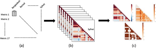
In the second step, we calculate the correlation of each pair of metrics for each network. Given that the aim of criticality analysis is to rank-order the transport network components, the empirical correlation should reflect the degree of similarity of the rankings produced by two metrics. Therefore, we use the Spearman-rank correlation coefficient. This coefficient focuses on the similarity of the ordering (i.e, ranking) of elements between any two sets, rather than on the actual values of the elements. A high and positive correlation coefficient between two metrics implies that both identify the similar set of links as critical.

In the third step, we check the robustness of the Spearman-rank correlation coefficients across all eight networks by using three indicators. The first indicator is the average of the coefficients, where a higher average indicates a more robust empirical similarity. However, this indicator by itself cannot detect outliers in the distribution. The second indicator, which is the range, addresses this issue. This indicator calculates the difference between the highest and the lowest correlation coefficients across the eight networks. If a pair of metrics has both a high average and a large range, then there may be some outliers in the empirical similarity. The third indicator checks for consistency in the direction of the empirical similarity. This consistency indicator follows a logical function where the value is one if the correlation coefficients of a pair of metrics are always negative (or positive) in all networks, and zero if the coefficients are negative in some networks but positive in the other networks.

4.3. Results of the empirical comparison

Figure 2 displays the robustness of the Spearman-rank correlations as heatmaps. The 17 criticality metrics are enlisted in both the x and y axes of the figure. Figure 2(a) shows that there are several metrics pairs that have very high positive correlation coefficients, while other pairs of metrics have negative correlation coefficients. Metric 11 (exposure to disaster) and metric 12 (availability of nearby alternative links) have low correlations to all other metrics. This implies that using these two metrics will yield unique sets of critical network components that cannot be found by using any of the other criticality metrics.

Figure 2. (a) Average, (b) Range, and (c) Consistency indicators of the correlation coefficients between all metrics pairs across the eight networks. The numbers on the axes corresponds to the metrics in Table 1.

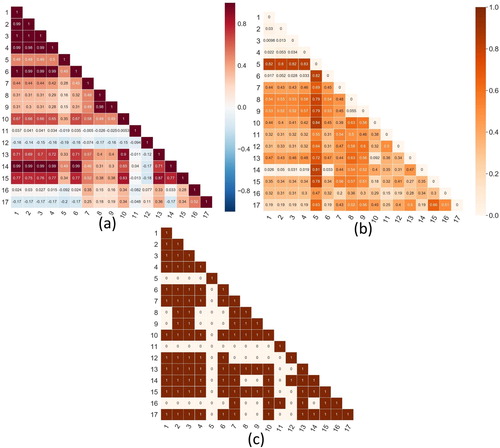
By comparing Figure 2(a) with Figure 2(b), we can see that metrics pairs that have high average correlation coefficients tend to have small ranges. Metric 5 (change in region-based unweighted total travel cost) has a unique, distinctive pattern. This metric has large ranges of correlation coefficients with all other metrics. This implies the degree of similarity between metric 5 and other metrics change substantially in different networks. Figure 2(c) shows the results of the consistency indicator. This figure indicates which pairs of metrics have inconsistent empirical similarity (negative correlation coefficients in some networks while positive in others). The consistency indicators for metric 5 and 11, for example, are always zero. This implies that the robustness of the empirical similarity of these metrics with all other metrics is very low, as the directions of the correlation coefficients change in different networks.

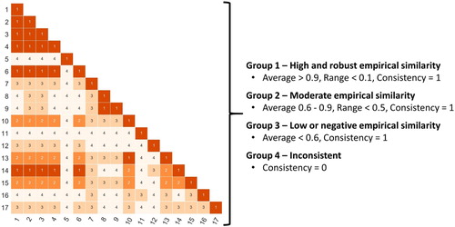
In Figure 3, we categorise the empirical similarity among the metrics based on the robustness indicators. Pairs of metrics that belong in group 1, such as metric 3 (change in worst-case user exposure) and metric 4 (change in unweighted total travel cost), have a high average correlation coefficient as well as a small range of correlation coefficients across the eight networks. This implies that metric 3 and 4 have high and stable empirical similarity, irrespective of the transport network for which they are calculated. If a metrics pair belongs to this category, we can just use one of the two metrics as they identify roughly the same set of links as critical. Metrics pairs in group 2 and group 3 have lower average and higher ranges of correlation coefficients. However, they are still consistent: the values of their coefficients are either always positive or always negative in all networks. In general, the degree of empirical similarity decreases from group 1 to group 4.

Figure 3. Grouping of empirical similarities among the metrics.

5. Discussion

5.1. Factors affecting correlation patterns between the networks

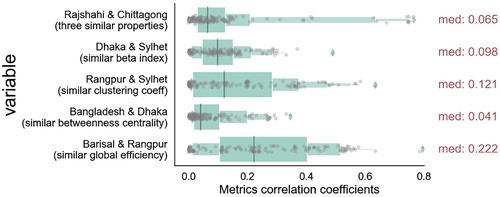
From a network theory point of view, it is important to identify the causes of the (dis)similarity of the metrics correlation patterns (i.e. the correlation heatmaps) across the eight networks. We can observe this by calculating the pairwise difference of the metrics correlation patterns between any two networks. If two networks have similar topological properties and similar correlation patterns, then we can say that these properties could explain the correlation patterns. We conduct pairwise comparisons for five pairs of networks, each pair sharing one similar topological property (see Table 2).

Figure 4 summarises the results of the pairwise comparisons. Note that each point in the figure represents a pairwise absolute difference of metrics correlation coefficients between two networks. Networks that have similar average betweenness centrality (Bangladesh and Dhaka networks) tend to produce similar correlation patterns. The analysis also shows that having similar global efficiency (Barisal and Rangpur networks) or similar clustering coefficient (Rangpur and Sylhet networks) results in dissimilar correlation patterns. Interestingly, networks having multiple similar topological properties (e.g. Rajshahi and Chittagong networks) have slightly less similar correlation patterns compared to networks having only average betweenness centrality in common (e.g. Bangladesh and Dhaka networks). Based on the Rajshahi and Chittagong networks, the effect of having similar beta index and similar average betweenness criticality counteracts the effect of having similar clustering coefficient.

Figure 4. Distribution of absolute difference in metrics correlation coefficients among several pairs of networks.

The average betweenness centrality can explain the similarity of the correlation patterns between the networks because assignment techniques are involved when one calculates some of the criticality metrics. These metrics are calculated in a way that is quite similar to average betweenness centrality, as both require the set of shortest paths between nodes. The difference is located in the set of nodes used for calculating the criticality metrics and the average betweenness centrality. In the former case, the representative centroid nodes of districts are used while in the latter case, all nodes in the network are considered.

The outlier points in Figure 4 indicate that even among networks with the most similar correlation patterns (i.e. Bangladesh and Dhaka), there are some metrics pairs that have substantially different correlation coefficients. This implies that the networks’ topological properties alone are insufficient for explaining the differences in the metrics’ correlations. Other non-network factors that may contribute to these differences are the spatial distribution of the OD nodes and the spatial distribution of the weight of production and attraction factors across these OD nodes. These non-network factors have a direct effect on the identification of the set of shortest paths, used in many of the criticality metrics. Consequently, we can expect that the correlation pattern may change if a different set of nodes is used as the centroid nodes, or if different production and attraction weights are given to these nodes. Regardless, future studies on understanding criticality metrics and their behaviour given topological characteristics of the underlying network would be a valuable research avenue.

Another factor that may play a role is the choice of the assignment techniques. The analysis in this study uses all-or-nothing assignment, resulting in only one shortest path between each pair of nodes. Using other techniques, such as congested assignment techniques, might result in a different set of shortest paths. This may not substantially influence correlation patterns between pairs of metrics that both require assignment techniques. For instance, if there are changes in the criticality scores of network components based on metric 1 (because we use congested assignment instead of all-or-nothing assignment), then the pattern of changes would be similar for metric 2, as long as both metrics require assignment techniques and are empirically similar in the first place. The choice of the assignment techniques, however, may slightly influence the correlation pattern between criticality metrics that require assignment techniques and those that do not.

5.2. Key findings from the empirical and the conceptual comparisons

One hypothesis made in the conceptual comparison is that criticality metrics that represent similar concepts would also have a high empirical similarity. We can evaluate this hypothesis on two levels: observing the empirical similarity among metrics that represent exactly the same concepts (within-category), and among metrics that represent different concepts (between-category). There are four possible outcomes: (i) whether two metrics have to share exactly the same three concepts in order to yield similar rankings, (ii) whether two metrics that share one or two (out of three) similar concepts may yield similar rankings, (iii) whether there is one dimension that strongly affects the empirical similarity of criticality metrics, or (iv) whether there is no relationships between the conceptual and empirical similarity.

5.2.1. Observation for the within-category

Rankings of network components from criticality metrics that share the same concepts are not necessarily highly correlated. For instance, both metric 15 and 16 (see Table 1) share the same concepts (connectivity – egalitarian – network-wide), but their degree of empirical similarity belongs to group 3 (low or negative empirical similarity, see Figure 3). The empirical similarity between metric 5 and 13 even belong to group 4 (inconsistent). There are also some metrics that have both conceptual and empirical similarity. Examples of these metrics are those that are based on travel cost, utilitarian, and network-wide aggregation concepts (metric 1, 2, and 3) and those with the travel cost, egalitarian, and network-wide aggregation concepts (metric 4 and 14). Nonetheless, this finding eliminates the first possibility discussed in the previous paragraph, as there are some metrics sharing the same concepts but having a low empirical similarity.

5.2.2. Observation for the between-category

There are four findings worth discussing from the between-category analysis. First, there is a high empirical similarity between metric 6 (accessibility – utilitarian – network-wide) and the network-wide travel cost metrics, regardless of the ethical dimension (metric 1, 2, 3, 4, and 14). This is the only high empirical similarity found between metrics that represent different functionalities.

Second, metrics that represent the travel cost functionality, and having a similar level of aggregation, tend to be highly correlated. Five metrics representing network-wide travel cost (metric 1, 2, 3, 4, and 14) have high and robust empirical similarity with each other. Adopting different ethical principles does not matter here. The same phenomenon applies to metrics based on local travel cost (metric 10 and 13). Hence, instead of calculating multiple metrics, we can simply use one metric and still reveal a similar critical links pattern on the network. This finding confirms the second possibility (metrics sharing some similar concepts would yield similar rankings), and thus eliminates the fourth possibility (no relationships between conceptual and empirical similarities).

Third, when comparing the results from travel cost metrics that share the same ethical principle but have different aggregation levels, lower correlations are found. The correlations can be moderately high, such as those between metric 13 and 14, metric 4 and 13, as well as metric 2 and 10. It can also be low (e.g. between metric 3 and 8) or even inconsistent (e.g. between metric 4 and 5). This implies that if transport authorities and/or analysts want to focus on the travel cost functionality, they can disregard the ethical dimension and focus on selecting the appropriate level of aggregation.

Fourth, except for the network-wide travel cost metrics, having an identical functionality concept and aggregation level but a different ethical principle results in low or inconsistent empirical similarity. This follows from observing the correlation between metric 5 and 6. Both metrics represent the network-wide accessibility concept, but the former adopts the utilitarian principle while the latter adopts the egalitarian principle. In Figure 3 we see that the empirical correlation between them belongs to the inconsistent group. Similar observations can be made regarding metric 8, 9, and 13 (local travel cost metrics), metric 15, 16, and 17 (network-wide connectivity metrics), as well as metric 11 and 12 (local connectivity metrics). This fact highlights the importance of the ethical principles. Transport authorities and/or analysts should carefully reflect on this both when selecting the criticality metrics to use and when deriving policy conclusions.

5.3. A guideline for selecting criticality metrics

We use the findings from the previous subsection to develop a guideline that can help transport authorities in choosing the appropriate criticality metrics to use. In line with the suggestion made by Jenelius and Mattsson (2015), the criticality metrics selection guideline follows a normative approach. The guideline consists of two steps. First, we have to categorise the policy problem that is being addressed. The three dimensions presented in the conceptual comparison can aid this process. Second, the set of metrics to use can be further narrowed down by observing the empirical dissimilarities among them.

Figure 5 details the two general steps described above into five steps. The first three steps require us to reflect on the three conceptual dimensions to be considered in the criticality analysis. The functionality dimension comes first, as the empirical analysis reveals that there is almost no empirical similarity found among metrics with different functionalities. If the travel cost functionality is selected, we can skip the ethical dimension and chooses the aggregation level directly (indicated by the dashed line in Figure 5). This is because travel cost metrics with the same aggregation level have high empirical similarity regardless of their ethical principles. For other functionalities, choosing the ethical principle comes before choosing the aggregation level. The fourth finding of the between-category observation underlies this ordering. The ethical dimension influences the empirical results more strongly compared to the aggregation dimension.

Figure 5. A five-step guideline to select criticality metrics.

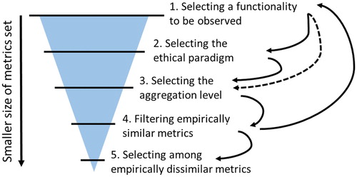
After making choices regarding functionality, ethical principles, and the level of aggregation, we can filter out metrics that are empirically similar (step 4 in Figure 5). For instance, if the network-wide and travel cost concepts are selected, we can select just one out of the five available metrics (metric 1, 2, 3, 4, and 14). In this case, selecting metrics with an egalitarian principle has practical advantages as they induce less computational cost. We may also want to evaluate more than one combination of conceptual dimensions. Accordingly, the first four steps are iterative. Once an exhaustive set of candidate metrics has been identified, the final step (step 5 in Figure 5) is performing a final check to ensure that there are no empirically similar metrics.

The empirical similarity grouping presented in Figure 3 serves as a basis to filter the candidate metrics in step 4 and 5 (see Figure 5). It is safe to assert that two metrics are highly empirically correlated if they belong to group 1, or that they are lowly correlated if they belong to either group 3 or 4. However, if the correlation of two metrics belongs to group 2, then the choice is left to the authorities and/or analysts. Practical considerations, such as data availability and computation cost, can help in making this choice.

5.4. Application of the guideline: a hypothetical policy problem

To demonstrate the application of the guideline, we propose the following hypothetical metrics selection problem for the Barisal Division of Bangladesh. Barisal Division is located in the south of the country. Having the smallest population size and lowest population density, Barisal Division is considered as one of the rural regions of Bangladesh. The division also has the shortest stretch of N and R roads in comparison to the other divisions. As the overall transport infrastructure network in this division is still in an earlier phase of the development, the transport authorities want to focus on providing adequate access to all towns within the division.

The first three steps of the guideline (see Figure 5) concern the selection of conceptual dimensions to be addressed: the functionality, ethical, and aggregation dimensions. The problem statement of the transport authorities indicates that the connectivity and the accessibility functionalities are the current concern. Choosing these functionalities requires one to select the ethical paradigm to be adopted. Based on the problem statement, the transport authorities are concerned with providing services to all towns, implying an egalitarian principle. We assume that both the local and the network-wide aggregations are considered since the problem statement does not touch upon this concern. Ideally, we would use a set of metrics that covers four combinations of conceptual dimensions. However, since there is no metrics identified in this study (see Table 1) that represents the accessibility – egalitarian – local concepts, in this hypothetical policy problem we only cover three combinations. Table 3 lists the four metrics that cover these three combinations.

Table 3. Spearman-rank correlation coefficients of criticality metrics for the Barisal division.

		Connectivity – Egalitarian – Network-wide		Connectivity – Egalitarian – Local	Accessibility – Egalitarian – Network-wide
		#15	#16	#12	#7
Connectivity – Egalitarian – Network-wide	#15	1	0.28	−0.23	0.28
	#16	0.28	1	0.064	0.26
Connectivity – Egalitarian – Local	#12	−0.23	0.064	1	0.054
Accessibility – Egalitarian – Network-wide	#7	0.28	0.26	0.054	1

The last two steps consist of identifying empirically similar metrics and retain metrics which are dissimilar since they highlight different sets of links as critical. Table 3 shows the rank correlation coefficients between the four accounted metrics. Because there is no pairs of metrics that has a high degree of empirical similarity, all metrics are kept in the final set of metrics for further deliberation with the transport authorities.

6. Conclusion

This paper conceptually and empirically compares seventeen widely used criticality metrics, identifies the relations between empirical and conceptual similarities across the metrics, and develops a guideline that helps in selecting an appropriate set of metrics. The guideline urges transport authorities and researchers to adopt a normative approach where they first have to explicitly delineate the specific aims of their analysis. The insights gained from both the conceptual and empirical comparisons were used to develop the guideline for selecting the appropriate metrics for a given policy question.

The conceptual comparison contrasted the seventeen metrics on three dimensions: transport functionality (either travel cost, connectivity, or accessibility), the ethical principles (utilitarian or egalitarian), and the level of aggregation (network-wide or localised). Each metric is characterised by these dimensions, while the concepts represented in each dimension may differ between metrics. The alternative concepts within each dimension may not be exhaustive yet. For instance, other ethical principles, such as sufficientarianism, have been considered to be relevant in transport studies (Lucas et al., 2016). However, we did not identify any criticality metric grounded in this principle.

The empirical comparison showed two irregularities in the correlations of the metrics’ results. First, the rank correlations varied across the 8 different networks. This variation could be attributed mainly to the topological properties of these networks. If criticality metrics are calculated for networks with similar average betweenness criticality and beta index, the rank correlations across the metrics are typically high. Second, after aggregating the correlations across the eight networks, we found that metrics representing the same combination of concepts did not necessarily yield similar rankings. Nevertheless, some patterns could still be observed. For instance, travel cost metrics with the same aggregation level were highly correlated, despite differences in the ethical principles.

The metrics selection guideline consists of two main steps. In the first step, transport authorities and/or analysts determine the aim of the criticality analysis based on the three conceptual dimensions. They have to select, in order, the transport functionality they are interested in, the underlying ethical principles, and the level of aggregation. This order is based on the empirical comparison where it is found that the functionality dimension is the most influential dimension in explaining low empirical similarity across metrics. Next, in the second step the remaining criticality metrics are further filtered based on their empirical similarity. It is unnecessary to calculate multiple metrics when the results of the calculations are expected to be the same.

The guideline can help transport authorities and/or analysts in making an informed choice for a set of criticality metrics. The guideline is systematic, as it starts with a conscious selection of transport-related concepts to be considered. The guideline is also efficient, as it can help its users in selecting metrics that require less data and computation without losing relevant insights. The guideline, however, is still semi-generic, as there may be other criticality metrics or conceptual dimensions not accounted for here. Nevertheless, the first stage of the guideline, which was founded on the conceptual comparison, is generic enough for selecting among other metrics that are not covered in this study.

Acknowledgements

The authors would like to thank World Bank Group, especially Julie Rozenberg and Cecilia Briceno-Garmendia, for their valuable inputs and feedbacks throughout the project.

Disclosure statement

No potential conflict of interest was reported by the authors.

ORCID

Bramka Arga Jafino http://orcid.org/0000-0001-6872-517X

Jan Kwakkel http://orcid.org/0000-0001-9447-2954

Alexander Verbraeck http://orcid.org/0000-0002-1572-0997

Additional information

Funding

This work is one of the outcomes of the project “Resilience of the Transport Network in Bangladesh: A graph-theoretical and simulation-based approach”, funded by the World Bank Korean Green Growth Trust Fund (KGGTF) from the World Bank Group.

References

- Aydin, N. Y., Casali, Y., Sebnem Duzgun, H., & Heinimann, H. R. (2019). Identifying changes in critical locations for Transportation networks using centrality. In S. Geertman, Q. Zhan, A. Allan, & C. Pettit (Eds.), Computational urban planning and Management for Smart Cities (pp. 405–423). New York: Springer International Publishing.
- Aydin, N. Y., Duzgun, H. S., Wenzel, F., & Heinimann, H. R. (2018). Integration of stress testing with graph theory to assess the resilience of urban road networks under seismic hazards. Natural Hazards, 91(1), 37–68. doi: 10.1007/s11069-017-3112-z
- Balijepalli, C., & Oppong, O. (2014). Measuring vulnerability of road network considering the extent of serviceability of critical road links in urban areas. Journal of Transport Geography, 39, 145–155. doi: 10.1016/j.jtrangeo.2014.06.025
- Bangladesh Bureau of Statistics. (2013). District statistics. http://www.bbs.gov.bd/site/page/2888a55d-d686-4736-bad0-54b70462afda/District-Statistics
- Baroud, H., Barker, K., Ramirez-Marquez, J. E., & Rocco, S. C. M. (2014). Importance measures for inland waterway network resilience. Transportation Research Part E: Logistics and Transportation Review, 62, 55–67. doi: 10.1016/j.tre.2013.11.010
- Berdica, K. (2002). An introduction to road vulnerability: What has been done, is done and should be done. Transport Policy, 9(2), 117–127. doi:10.1016/S0967-070X(02)00011-2.
- Chen, B. Y., Lam, W. H. K., Sumalee, A., Li, Q., & Li, Z.-C. (2012). Vulnerability analysis for large-scale and congested road networks with demand uncertainty. Transportation Research Part A: Policy and Practice, 46(3), 501–516. doi: 10.1016/j.tra.2011.11.018
- Chen, A., Yang, C., Kongsomsaksakul, S., & Lee, M. (2007). Network-based accessibility measures for vulnerability analysis of degradable transportation networks. Networks and Spatial Economics, 7(3), 241–256. doi: 10.1007/s11067-006-9012-5
- Dehghani, M. S., Flintsch, G., & McNeil, S. (2014). Impact of road conditions and disruption uncertainties on network vulnerability. Journal of Infrastructure Systems, 20, 04014015. doi: 10.1061/(ASCE)IS.1943-555X.0000205
- Delbosc, A., & Currie, G. (2011). Using Lorenz curves to assess public transport equity. Journal of Transport Geography, 19(6), 1252–1259. doi: 10.1016/j.jtrangeo.2011.02.008
- Demirel, H., Kompil, M., & Nemry, F. (2015). A framework to analyze the vulnerability of European road networks due to Sea-level Rise (SLR) and sea storm surges. Transportation Research Part A: Policy and Practice, 81, 62–76. doi: 10.1016/j.tra.2015.05.002
- De Oliveira, E. L., da Silva Portugal, L., & Junior, W. P. (2016). Indicators of reliability and vulnerability: Similarities and differences in ranking links of a complex road system. Transportation Research Part A: Policy and Practice, 88, 195–208.
- Du, Q., Kishi, K., Aiura, N., & Nakatsuji, T. (2014). Transportation network vulnerability: Vulnerability Scanning Methodology applied to multiple Logistics transport networks. Transportation Research Record: Journal of the Transportation Research Board, 2410, 96–104. doi: 10.3141/2410-11
- Faturechi, R., & Miller-Hooks, E. (2014). Measuring the performance of transportation infrastructure systems in disasters: A comprehensive review. Journal of Infrastructure Systems, 21(1). doi: 10.1061/(ASCE)IS.1943-555X.0000212
- Ford, L. R., & Fulkerson, D. R. (1956). Maximal flow through a network. Canadian Journal of Mathematics, 8(3), 399–404. doi: 10.4153/CJM-1956-045-5
- Gauthier, P., Furno, A., & El Faouzi, N.-E. (2018). Road network resilience: How to identify critical links Subject to Day-to-Day disruptions. Transportation Research Record, 2672(1), 54–65. doi: 10.1177/0361198118792115
- Hansen, W. G. (1959). How accessibility shapes land use. Journal of the American Institute of Planners, 25(2), 73–76. doi: 10.1080/01944365908978307
- Hernández, L. G., & Gómez, O. G. (2011). Identification of critical segments by vulnerability for freight transport on the paved road network of Mexico. Investigaciones Geográficas, 74, 48–57.
- Issacharoff, L., Lämmer, S., Rosato, V., & Helbing, D. (2008). Critical infrastructures vulnerability: The highway networks. In D. Helbing (Ed.), Managing complexity: Insights, concepts, applications (pp. 201–216). Heidelberg: Springer-Verlag Berlin Heidelberg.
- Ivanova, O. (2014). Modelling inter-regional freight demand with input–output, gravity and SCGE methodologies. In L. Tavasszy & G. De Jong (Eds.), Modelling freight transport (pp. 13–42). Netherlands: Elsevier.
- Jenelius, E. (2009). Network structure and travel patterns: Explaining the geographical disparities of road network vulnerability. Journal of Transport Geography, 17(3), 234–244. doi: 10.1016/j.jtrangeo.2008.06.002
- Jenelius, E., & Mattsson, L.-G. (2015). Road network vulnerability analysis: Conceptualization, implementation and application. Computers, Environment and Urban Systems, 49, 136–147. doi: 10.1016/j.compenvurbsys.2014.02.003
- Jenelius, E., Petersen, T., & Mattsson, L.-G. (2006). Importance and exposure in road network vulnerability analysis. Transportation Research Part A: Policy and Practice, 40(7), 537–560.
- Kermanshah, A., & Derrible, S. (2016). A geographical and multi-criteria vulnerability assessment of transportation networks against extreme earthquakes. Reliability Engineering & System Safety, 153, 39–49. doi: 10.1016/j.ress.2016.04.007
- Knoop, V. L., Snelder, M., van Zuylen, H. J., & Hoogendoorn, S. P. (2012). Link-level vulnerability indicators for real-world networks. Transportation Research Part A: Policy and Practice, 46(5), 843–854. doi: 10.1016/j.tra.2012.02.004
- Koks, E. E., Rozenberg, J., Zorn, C., Tariverdi, M., Vousdoukas, M., Fraser, S. A., … Hallegatte, S. (2019). A global multi-hazard risk analysis of road and railway infrastructure assets. Nature Communications, 10(1), 2677. doi: 10.1038/s41467-019-10442-3
- Kurauchi, F., Uno, N., Sumalee, A., & Seto, Y. (2009). Network evaluation based on connectivity vulnerability. In W. H. K. Lam, H. Wong, & H. K. Lo (Eds.), Transportation and traffic theory 2009: Golden Jubilee (pp. 637–649). New York, USA: Springer US.
- Lakshmanan, T. R. (2011). The broader economic consequences of transport infrastructure investments. Journal of Transport Geography, 19(1), 1–12. doi: 10.1016/j.jtrangeo.2010.01.001
- Latora, V., & Marchiori, M. (2001). Efficient behavior of small-world networks. Physical Review Letters, 87(19). doi: 10.1103/PhysRevLett.87.198701
- Lin, J., & Ban, Y. (2013). Complex network topology of transportation systems. Transport Reviews, 33(6), 658–685. doi: 10.1080/01441647.2013.848955
- Litman, T. (2007). Developing indicators for comprehensive and sustainable transport planning. Transportation Research Record, 2017(1), 10–15. doi: 10.3141/2017-02
- Luathep, P., Sumalee, A., Ho, H. W., & Kurauchi, F. (2011). Large-scale road network vulnerability analysis: A sensitivity analysis based approach. Transportation, 38(5), 799–817. doi: 10.1007/s11116-011-9350-0
- Lucas, K., van Wee, B., & Maat, K. (2016). A method to evaluate equitable accessibility: Combining ethical theories and accessibility-based approaches. Transportation, 43(3), 473–490. doi: 10.1007/s11116-015-9585-2
- Martens, K., Bastiaanssen, J., & Lucas, K. (2019). Measuring transport equity: Key components, framings and metrics. In K. Lucas, K. Martens, F. Di Ciommo, & A. Dupont-Kieffer (Eds.), Measuring transport equity (pp. 13–36). The Netherlands: Elsevier.
- Mattsson, L.-G., & Jenelius, E. (2015). Vulnerability and resilience of transport systems – A discussion of recent research. Transportation Research Part A: Policy and Practice, 81, 16–34. doi: 10.1016/j.tra.2015.06.002
- Miller, E. J. (2018). Accessibility: Measurement and application in transportation planning. Transport Reviews, 38(5), 551–555. doi: 10.1080/01441647.2018.1492778
- Mishra, S., Welch, T. F., & Jha, M. K. (2012). Performance indicators for public transit connectivity in multi-modal transportation networks. Transportation Research Part A: Policy and Practice, 46(7), 1066–1085. doi: 10.1016/j.tra.2012.04.006
- Morris, J. M., Dumble, P. L., & Wigan, M. R. (1979). Accessibility indicators for transport planning. Transportation Research Part A: General, 13(2), 91–109. doi: 10.1016/0191-2607(79)90012-8
- Nagae, T., Fujihara, T., & Asakura, Y. (2012). Anti-seismic reinforcement strategy for an urban road network. Transportation Research Part A: Policy and Practice, 46(5), 813–827. doi: 10.1016/j.tra.2012.02.005
- Nagurney, A., & Qiang, Q. (2008). A network efficiency measure with application to critical infrastructure networks. Journal of Global Optimization, 40(1), 261–275. doi: 10.1007/s10898-007-9198-1
- Nahmias-Biran, B.-h., Martens, K., & Shiftan, Y. (2017). Integrating equity in transportation project assessment: A philosophical exploration and its practical implications. Transport Reviews, 37(2), 192–210. doi: 10.1080/01441647.2017.1276604
- Nourzad, S. H. H., & Pradhan, A. (2016). Vulnerability of infrastructure systems: Macroscopic analysis of critical disruptions on road networks. Journal of Infrastructure Systems, 22(1). doi: 10.1061/(ASCE)IS.1943-555X.0000266
- Pant, R., Hall, J. W., & Blainey, S. P. (2016). Vulnerability assessment framework for interdependent critical infrastructures: Case-study for Great Britain’s rail network. European Journal of Transport and Infrastructure Research, 16(1), 174–194.
- Pazner, E. A., & Schmeidler, D. (1978). Egalitarian equivalent allocations: A new concept of economic equity. The Quarterly Journal of Economics, 92(4), 671–687. doi: 10.2307/1883182
- Pereira, R. H. M., Schwanen, T., & Banister, D. (2016). Distributive justice and equity in transportation. Transport Reviews, 37(2), 170–191. doi: 10.1080/01441647.2016.1257660
- Posner, R. A. (1979). Utilitarianism, economics, and legal theory. The Journal of Legal Studies, 8(1), 103–140. doi: 10.1086/467603
- Qi, W., Zhang, Z., Zheng, G., & Lin, X. (2015). Vertex importance analysis of Xiamen road transportation networks. Journal of Information and Computational Science, 12(10), 3927–3936. doi: 10.12733/jics20105979
- Qiang, P., & Nagurney, A. (2012). A bi-criteria indicator to assess supply chain network performance for critical needs under capacity and demand disruptions. Transportation Research Part A: Policy and Practice, 46(5), 801–812. doi: 10.1016/j.tra.2012.02.006
- Reggiani, A., Nijkamp, P., & Lanzi, D. (2015). Transport resilience and vulnerability: The role of connectivity. Transportation Research Part A: Policy and Practice, 81, 4–15. doi: 10.1016/j.tra.2014.12.012
- Rietveld, Piet. (1994). Spatial economic impacts of transport infrastructure supply. Transportation Research Part A: Policy and Practice, 28(4), 329–341. doi:10.1016/0965-8564
- Scott, D. M., Novak, D. C., Aultman-Hall, L., & Guo, F. (2006). Network robustness index: A new method for identifying critical links and evaluating the performance of transportation networks. Journal of Transport Geography, 14(3), 215–227. doi: 10.1016/j.jtrangeo.2005.10.003
- Shier, D. R. (1979). On algorithms for finding the k shortest paths in a network. Networks, 9(3), 195–214. doi: 10.1002/net.3230090303
- Smith, G. (2009). Bangladesh transport policy Note. Washington, DC: World Bank. Retrieved from http://siteresources.worldbank.org/INTSARREGTOPTRANSPORT/Resources/BD-Transport-PolicyNote_9June2009.pdf
- Snelder, M., van Zuylen, H. J., & Immers, L. H. (2012). A framework for robustness analysis of road networks for short term variations in supply. Transportation Research Part A: Policy and Practice, 46(5), 828–842. doi: 10.1016/j.tra.2012.02.007
- Sohn, J. (2006). Evaluating the significance of highway network links under the flood damage: An accessibility approach. Transportation Research Part A: Policy and Practice, 40(6), 491–506. doi: 10.1016/j.tra.2005.08.006
- Sullivan, J., Aultman-Hall, L., & Novak, D. (2009). A review of current practice in network disruption analysis and an assessment of the ability to account for isolating links in transportation networks. Transportation Letters, 1(4), 271–280. doi: 10.3328/TL.2009.01.04.271-280
- Sullivan, J. L., Novak, D. C., Aultman-Hall, L., & Scott, D. M. (2010). Identifying critical road segments and measuring system-wide robustness in transportation networks with isolating links: A link-based capacity-reduction approach. Transportation Research Part A: Policy and Practice, 44(5), 323–336.
- Taylor, M. A. P., & D’Este, G. M. (2007). Transport network vulnerability: A method for diagnosis of critical locations in transport infrastructure systems. In A. T. Murray, & T. H. Grubesic (Eds.), Critical infrastructure: Reliability and vulnerability (pp. 9–30). Berlin, Heidelberg: Springer Berlin Heidelberg.
- Thomopoulos, N., Grant-Muller, S., & Tight, M. R. (2009). Incorporating equity considerations in transport infrastructure evaluation: Current practice and a proposed methodology. Evaluation and Program Planning, 32(4), 351–359. doi: 10.1016/j.evalprogplan.2009.06.013
- Ureña, J. M., Menerault, P., & Garmendia, M. (2009). The high-speed rail challenge for big intermediate cities: A national, regional and local perspective. Cities, 26(5), 266–279. doi: 10.1016/j.cities.2009.07.001
- Van Wee, B., & Roeser, S. (2013). Ethical Theories and the cost–benefit analysis-based ex ante evaluation of transport policies and plans. Transport Reviews, 33(6), 743–760. doi: 10.1080/01441647.2013.854281
- Velaga, N. R., Beecroft, M., Nelson, J. D., Corsar, D., & Edwards, P. (2012). Transport poverty meets the digital divide: Accessibility and connectivity in rural communities. Journal of Transport Geography, 21, 102–112. doi:j.jtrangeo.2011.12.005 doi: 10.1016/j.jtrangeo.2011.12.005
- Wang, Z., Chan, A. P. C., & Li, Q. (2014). A critical review of vulnerability of transport networks: From the perspective of complex network. In J. Wang, Z. Ding, L. Zou, & J. Zuo (Eds.), Proceedings of the 17th international symposium on advancement of construction management and real estate (pp. 897–905). Heidelberg: Springer-Verlag Berlin Heidelberg.
- Wang, Y., & Cullinane, K. (2014). Traffic consolidation in East Asian container ports: A network flow analysis. Transportation Research Part A: Policy and Practice, 61, 152–163. doi: 10.1016/j.tra.2014.01.007
- Wang, J., Jin, F., Mo, H., & Wang, F. (2009). Spatiotemporal evolution of China’s railway network in the 20th century: An accessibility approach. Transportation Research Part A: Policy and Practice, 43(8), 765–778. doi: 10.1016/j.tra.2009.07.003
- Zhou, Y., Fang, Z., Thill, J.-C., Li, Q., & Li, Y. (2015). Functionally critical locations in an urban transportation network: Identification and space–time analysis using taxi trajectories. Computers, Environment and Urban Systems, 52, 34–47. doi: 10.1016/j.compenvurbsys.2015.03.001