Extended Kalman filtering for fuzzy modelling and multi-sensor fusion

Abstract

Extended Kalman Filtering (EKF) is proposed for: (i) the extraction of a fuzzy model from numerical data; and (ii) the localization of an autonomous vehicle. In the first case, the EKF algorithm is compared to the Gauss–Newton nonlinear least-squares method and is shown to be faster. An analysis of the EKF convergence is given. In the second case, the EKF algorithm estimates the state vector of the autonomous vehicle by fusing data coming from odometric sensors and sonars. Simulation tests show that the accuracy of the EKF-based vehicle localization is satisfactory.

Keywords:

• Extended Kalman filtering
• Fuzzy modelling
• Gauss–Newton method
• Vehicle localization
• Multi-sensor fusion

1. Introduction

The Extended Kalman Filter (EKF) is an incremental estimation algorithm that performs optimization in the least-mean-squares sense and has been successfully applied to neural networks training and to data-fusion problems. In this paper, the EKF is employed for: (i) the extraction of a fuzzy model from numerical data; and (ii) for the localization of an autonomous vehicle by fusing data coming from odometric and sonar sensors.

In the first case, the EKF algorithm is used to estimate the parameters of a fuzzy model that approximates a nonlinear surface. It is known that the EKF algorithm is particularly successful compared to first-order gradient-descent methods with error back-propagation 1. In this paper, it is shown that EKF training is also faster than second-order gradient methods such as the pure Gauss–Newton algorithm. The EKF does not wait to process the entire data set before updating the parameter estimates . Instead, it processes the data incrementally and updates after each training example is picked. Thus, the method is suitable for large data sets and real-time operation 2,3. In the second case, the EKF is used for the localization of an autonomous vehicle that moves in a workspace defined by planar surfaces 4. The EKF performs fusion of the data that come from odometric and sonar sensors. EKF-based sensor fusion provides satisfactory localization of the mobile robot and enables the application of nonlinear steering control.

The structure of the paper is as follows. In Section 2, common methods for fuzzy model estimation are presented. The Gauss–Newton method for nonlinear least-squares identification is explained. In Section 3, nonlinear estimation with the use of EKF is presented. In Section 4, the problem of data fusion with the use of EKF is analysed. EKF-based data fusion for vehicle localization is introduced. In Section 5, simulation tests are provided. The EKF algorithm is used for the estimation of a nonlinear model as well as for the localization of an autonomous vehicle with the use of data from different sensors. Finally, in Section 6, concluding remarks are stated.

2 Fuzzy modelling issues

2.1 Local linear fuzzy models

Assume that data from an unknown function y = f(x ₁, x ₂, …, x_n ) are observed. The aim is to use these data to construct an appoximation [fcirc](x ₁, x ₂, …, x_n ). In fuzzy modelling [fcirc](x) is represented as a collection of fuzzy IF – THEN rules. The Takagi–Sugeno rule-base model is considered 5:

where l = 1, 2, …, L, R^l is the lth rule, x = [x ₁, x ₂, …, x_n ] ^T is the input (IF) variable, y is the output (THEN) variable, and , b ^l are the parameters of the local linear models. The output is calculated by taking the weighted average of the rules THEN part , where : R → [0, 1] is the membership function of the fuzzy set in the antecedent part of the rule R^l . The centres of the fuzzy sets are denoted as . The corresponding widths are assumed to be known constants. The concept of local linear fuzzy models can also be extended to the modelling of dynamical systems.

2.2 Common methods for fuzzy model estimation

Parameter estimation using the backpropagation algorithm can be slow. Thus, nonlinear least-squares methods, such as Gauss–Newton, Levenberg–Marquardt and the Extended Kalman Filter (EKF) are more suitable 5. It is assumed that parameters of the nonlinear system do not change with time. Thus, the parameters vector of the physical system measured at instant k − 1 is θ(k − 1) and equals the parameters vector measured at instant k. Therefore, θ(k) = θ(k − 1). It is also assumed that the order of the physical system and of the fuzzy model is the same, i.e. they contain the same number of parameters. Finally, the following notation is used: y(k) is the output of the fuzzy model at instant k, x(k) is the input vector of the fuzzy model at instant k, and d(k) is the output of the physical system at instant k. The difference between d(k) and y(k) is denoted by e(k).

The Gauss–Newton method uses a Taylor series expansion to approximate the nonlinear model and then employs ordinary least squares to estimate the model's parameters:

where j denotes the jth parameter and k the kth iteration of the algorithm. The cumulative quadratic error is , where r(k) is the difference y((k − 1), x(k)) − d(k), J is the Jacobian matrix of the output with respect to the parameters vector θ, and θ(k) − (k − 1) is the difference between the current and the estimated previous value of the parameter vector.

The derivative of E with respect to θ is . The minimum condition gives the parameters update law

where λ is a non-negative parameter. It has to be noted that in the Gauss–Newton method, the data are processed in batch mode, i.e. the parameter estimates are updated at the end of each epoch (g ₁, g ₂, …, g_N ). On the other hand, in the EKF case, the training data are processed sequentially.

3 Fuzzy model estimation using EKF

The EKF was initially conceived as a method for estimating parameters from nonlinear measurements that are generated in real time. The basic idea of the method is to linearize each new measurement around the current value of the estimate and treat the measurement as if it was linear. The EKF for fuzzy models generation is a generalization of the well-known Recursive Least Squares (RLS) algorithm 6. The same assumptions about the nonlinear system and its fuzzy model as in Section 2.2 are made. The extended Kalman filter equations are derived by expanding the nonlinear function around the current estimate parameter vector. This means that at each step of the algorithm, the regressor vector is substituted by the gradient of the estimated output, i.e.

where , and ρ(k) are the higher-order terms of the Taylor expansion. In a state model form, one gets:

where ξ(k) is . The parameters vector θ(k) is estimated by the following recursion

where λ is the so-called ‘forgetting factor’, K is the Kalman gain and P is the inverse of the correlation matrix of J. The algorithm can be initialized with P(0) = αI, α > 0 and to some nonzero random value. The EKF is an incremental parameter estimation algorithm since it performs an update of θ for every new training pattern x_i , y_i , i = 1, …, n.

3.1 Fuzzy model estimation using EKF

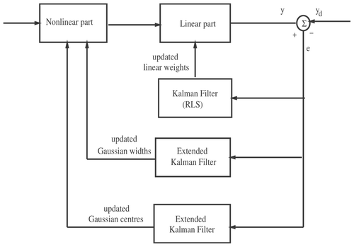
The block diagram of the EKF training is shown in figure 1. In the case of a fuzzy model, there are three groups of parameters to be learned from the numerical data: the linear weights, the nonlinear centres, and the nonlinear spreads 7.

Figure 1. EKF block diagram.

To reduce computation overhead, which is due to large matrix dimensionality, three separate Kalman filter algorithms are employed, i.e. for the calculation of the linear weights, centres and spreads of the membership functions, respectively.

Step 1: Optimizing the linear weights . Since the parameters are linear, the elements of the gradient matrix J_w of the parameters appearing in the THEN part of the rule are

The update laws of the algorithm are given by equation 5, setting and .

Step 2: Optimizing the centres of the membership functions. The gradient with respect to the centre is

The centres update is given by equation (5), setting and .

Step 3: Optimizing the spreads of the membership functions. The gradient with respect to the spread is

The spreads update is given by equation (5), setting and .

4 Data fusion with the use of extended Kalman filtering

The paper will also investigate the application of EKF to the fusion of data that come from different sensors. Sensor fusion algorithms can be classified into three different groups: (i) fusion based on probabilistic models; (ii) fusion based on least-squares techniques (e.g. Kalman Filtering); and (iii) intelligent fusion (e.g. fuzzy logic) 8. This paper is concerned with case (ii).

4.1 Review of the Kalman filter for the linear state-measurement model

A dynamical system is assumed to be expressed in the form of a state model 9:

where the state x(k) is an N-vector, w(k) is an N-element process noise vector, Φ is an N × N real matrix, C is an N-element row vector of real numbers, and v(k) is the measurement noise. It is assumed that w(k) and v(k) are uncorrelated.

Now, the problem of interest is to estimate the state x(k) based on the measurements z(1), z(2), …, z(k). Actually, this is a linear minimum-mean-squares estimation problem (LMMSE) which is solved recursively, i.e. ◯(k + 1) = a _n+1 (◯ (k), z(k + 1)). The process and output noise are white, and their covariance matrices are given by: E[w(i)w^T (j)] = Qδ (i − j) and E[v(i)v^T (j)] = Rδ (i − j). The initial value of the state vector x(0), the initial value of the error covariance matrix P(0), is unknown, and an estimation of it is considered, i.e. ◯(0) = a guess of E[x(0)], and [Pcirc](0) = a guess of Cov[x(0)]. For the initialization of matrix P, one can set [Pcirc] (0) = λI, with λ > 0.

The Kalman filter can be broken down into two parts: (i) time update and (ii) measurement update. The first part employs an estimate ◯ ⁻(k) of the state vector x(k) made before the output measurement z(k) is available (a priori estimate), i.e. when the set of measurements is Z ⁻ = lcub;z(1), …, z(k − 1)rcub;. The second part provides an estimate ◯(k) of x(k) after z(k) has become available (a posteriori estimate), when the set of measurements becomes Z = lcub;z(1), …, z(k)rcub;.

The associated estimation errors are defined by e ⁻(k) = x(k) − ◯ ⁻(k) = the a priori error, and e(k) = x(k) − ◯(k) = the a posteriori error. The estimation error covariance matrices associated with ◯ ⁻(k) and ◯(k) are P ⁻(k) = Cov[e ⁻(k)] = E[e ⁻(k)e ⁻(k) ^T ] and P(k) = Cov[e(k)] = E[e(k)e ^T (k)]. From the definition of the trace of a matrix, the mean-square error of the estimates can be written as MSE(◯ ⁻(k)) = E[e ⁻(k)e ⁻(k) ^T ] = tr(P ⁻(k)) and MSE(x(k)) = E[e(k)e ^T (k)] = tr(P(k)). Finally, the linear Kalman filter equations are equivalent to equation (5).

Measurement update:

Time update:

4.2 Extended Kalman filter for the nonlinear state-measurement model

The following nonlinear time-invariant state model is now considered 9:

where w(k) and v(k) are uncorrelated, zero-mean, white noise processes with covariance matrices Q(k) and R(k), respectively. The operators φ(x) and γ(x) are given by φ(x) = [φ₁(x), φ₂(x), …, φ _m (x)]T, and γ(x) = [γ₁(x), γ₂(x), …, γ _P (x)] ^T , respectively. It is assumed that φ and γ are sufficiently smooth in x so that each has a valid series Taylor expansion. Following the linearization procedure presented in Section 3, φ is expanded into Taylor series about ◯:

where J _φ(x) is the Jacobian of φ calculated at ◯(k):

Likewise, γ is expanded about ◯ ⁻(k)

where ◯ ⁻(k) and ◯(k) were defined in Section 4.1. The Jacobian J _γ(x) is

The resulting expressions create first-order approximations of φ and γ. Thus, the linearized version of the plant is obtained:

Now, the EKF recursion is stated as in equations (10) and (11). First, the time update is considered: the estimation of the state vector at instant k is denoted by ◯(k). Given initial conditions ◯ ⁻ (0) and P ⁻(0), the recursion proceeds as:

	Measurement update: Acquire z(k) and compute
	Time update: Compute

From equation (17), it can be seen that J _γ denotes C, while from equation (18), it can be seen that J _φ denotes Φ given in equation (9).

4.3 EKF-based data fusion for vehicle localization

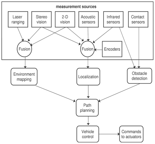
The role of multi-sensor fusion for mobile robot localization is shown in figure 2. Systems for vehicle localization can be classified in two main categories 4:

	Relative localization, which is realized through sensors measuring internal parameters of the vehicle, such as position, velocity, and angular velocity. Typical internal sensors are optical incremental encoders, which are fixed to the axes of the driving wheels and the steering axis of the vehicle.
	Absolute localization, which is performed using sensors that collect data from the vehicle's environment. A set of sonars is generally used as external sensor devices. Sonars are fixed to the vehicle and measure the distance with respect to obstacles and surfaces in its workspace.

The combination of acoustic and odometric sensors for mobile robot localization is a well-established approach. Compared with visual sensors, sonar are more credible when the robot moves in an environment of changing light conditions. Moreover, sonar are preferred to laser sensors when energy sources are of limited capacity.

Figure 2. Multi-sensor fusion in mobile robot navigation.

Encoder measurements are prone to error accumulation and therefore introduce uncertainty in the vehicle's localization. Moreover, distance measurements from acoustic sensors are subject to uncertainty, which is expected to be significant when the measurement is taken far from the landmarks. Sonar measurements may be affected by white Gaussian noise and also by crosstalk interferences and multiples echoes. Extended Kalman Filtering is used to fuse the measurements from the various sensors as the robot moves, and statistically minimize the error in the estimation of the vehicle's state vector.

5 Simulation results

5.1 Fuzzy model estimation using EKF

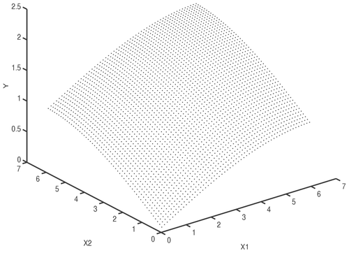
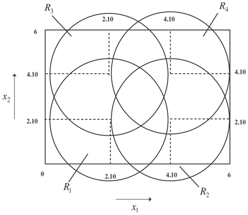
EKF was employed to extract fuzzy rules from numerical data. The function y = sin(0.25x ₁) + sin(0.25x ₂) was used as a test case ( figure 3). The training set contained N = 3000 noise-free triplets (x _1i , x _2i , y, i = 1,…, 3000). The input vector [x ₁, x ₂] ^T was uniformly distributed in the interval [0, 6] × [0, 6]. Following the analysis in Section 2.1, the nonlinear surface was approximated by four local models. The centres of these local models and j = 1, 2, 3, 4 were initialized as follows: , , , , , , . The spread of the membership functions is denoted by v and was set to v = 3. The parameters appearing in the THEN part were all initialized to 0. After training, the following rules were identified (figure 4):

Figure 3. Nonlinear function approximated by the fuzzy model.

Figure 4. Fuzzy-rule base generated with input space partitioning.

Remark

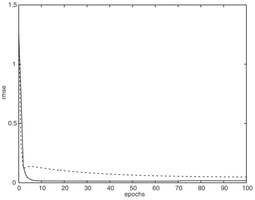
Regarding convergence, it is known that the speed of EKF training is better than that of the LMS algorithm 3. Our simulation tests show that the EKF is also faster than the pure Gauss–Newton method due to setting λ < 1 in the initial training cycles. This is demonstrated in figure 5.

Figure 5. RMSE of the EKF (continuous line) and the Gauss–Newton (dashed line) algorithm.

The EKF algorithm resembles asymptotically to a gradient method with diminishing stepsize. It has been proved (2,3) that for λ = 1 and for a large number of learning steps k, the EKF iteration can be written approximately as

which is an approximation of the Gauss–Newton iteration with diminishing step size. The RMSE decrease in the EKF algorithm tends to be faster when λ < 1, because in that case, the implicit step size does not diminish as in the case of λ = 1. If λ < 1, the effect of old data is discounted, and successive estimates produced by the method tend to change faster. However, when λ < 1, the matrix P(k) in the EKF recursion of equation (5) does not assure convergence. Thus, for a rapid decrease in RMSE without any risk of divergence, one may start with a relatively small λ and raise it progressively to 1. The tuning of λ is based on heuristics. In 2, a proposition for the selection of λ is presented:

Proposition

It is assumed that the Jacobian matrix J(θ, x) is full rank and that for some L > 0 || J_i (x)y(θ, x) – J_i (x′)y(0,x′) || ⩽ L || x – x′ ||, ∀x, x′ ∈ R ⁿ holds, where J_i with i = 1, 2, …, N is the ith row of the Jacobian matrix, which is associated with the ith training sample. If, for the constant c > 0, the forgetting factor λ_q , at the qth epoch, satisfies , then the EKF converges. This proposition demonstrates that as the number of epochs q increases and , the convergence condition is λ_q  → 1.

In the simulation tests, the initial value of λ was chosen to be 0.999. It is known that the memory of the RLS algorithm is approximated by . Since the EKF consists of local RLS algorithms, choosing λ = 0.999 means that only 1000 out of the 3000 triplets g_i are taken into account in the first steps of the EKF training. This explains why the EKF algorithm converges faster than the Gauss–Newton method. An oscillatory behaviour of the algorithm and possible divergence can be avoided if the gain λ is progressively raised to 1. After 200 epochs, the RMSE of the EKF algorithm was 1.4e – 2. In the case of the Gauss–Newton method, the RMSE obtained after 200 epochs was 4.43e – 2. To reduce the RMSE further, a greater number of local fuzzy models is required.

5.2 EKF-based sensor fusion for autonomous vehicle localization

A unicycle robot is considered. Its continuous-time kinematic equation is given by

which is a simplified model of a car-like robot studied in 10,11. Encoders are placed on the driving wheels and provide a measure of the incremental angles over a sampling period Δt_k . These odometric sensors are used to obtain an estimation of the displacement and the angular velocity of the vehicle v(t) and ω(t), respectively. These encoders introduce incremental errors, which result in an erroneous estimation of the orientation θ. To improve the accuracy of the vehicle's localization, measurements from sonars can be used. The distance measure of sonar i from the neighbouring surface P_j is taken into account (see figures 6 and 7).

Figure 6. Mobile robot with odometric sensors.

Figure 7. Orientation of the sonar i.

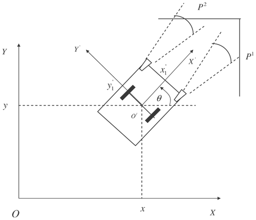
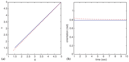
The inertial coordinates system OXY is defined. Furthermore, the coordinates system O′X′Y′ is considered ( figure 6). O′X′Y′ results from OXY if it is rotated by an angle θ (figure 6). The coordinates of the centre of the wheels axis with respect to OXY are (x, y), while the coordinates of the sonar i that is mounted on the vehicle, with respect to O′X′Y′, are x _i ′, y _i ′. The orientation of the sonar with respect to OX′Y′ is θ _i ′. Thus, the coordinates of the sonar with respect to OXY are (x_i , y_i ), and its orientation is θ_i with

Each plane P^j in the robot's environment can be represented by and ( figure 7), where (i) is the normal distance of the plane from the origin O, and (ii) is the angle between the normal line to the plane and the x-direction.

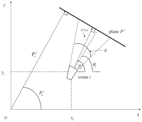
The sonar i is at position x_i (k), y_i (k) with respect to the inertial coordinates system OXY, and its orientation is θ_i (k). Using the above notation, the distance of the sonar i, from the plane P^j is represented by , (see figure 7):

if , where δ is the width of the sonar beam. Assuming a constant sampling period Δt_k  = T, the measurement equation is z(k + 1) = γ(x(k)) + v(k), where z(k) is the vector containing sonar and odometer measures and v(k) is a white noise sequence ∼N(0, R(kT)). The dimension p_k of z(k) depends on the number of sonar sensors. The measure vector z(k) can be decomposed in two subvectors

with i = 1, 2, …, n _s, where n _s is the number of sonars, is the distance measure with respect to the plane P ^j provided by the ith sonar and j = 1, …, n _p where n _p is the number of surfaces. By definition of the measurement vector, the output function γ(x(k)) is given by . The robot state is [x(k), y(k), θ(k)] ^T , and the control input is denoted by U(k) = [u(k), ω(k)] ^T .

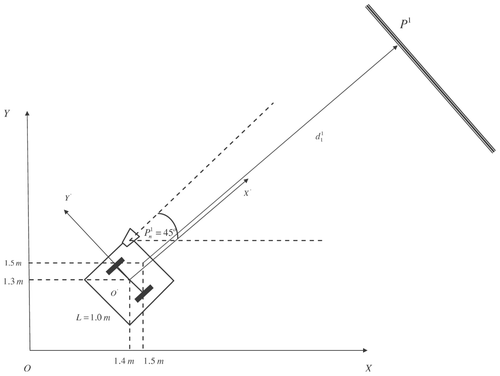
In this simulation test, the number of sonar is taken to be n _s = 1, and the number of planes n _p = 1, so the measurement vector becomes . The extended Kalman Filter (EKF) is obtained if the kinematic model of the vehicle is linearized about the estimates ◯(k) and ◯ ⁻(k) and the control input U(k) is applied.

The measurement update of the EKF is

The time update of the EKF is

where

with σ ²(k) chosen to be 10⁻³ and ,

Assuming 1 sonar n _s = 1, and one plane P ¹, n _p = 1 one has , i.e.

The vehicle is steered by a dynamic feedback linearization control algorithm which is based on PD control 12:

The following initialization is assumed (see figure 8):

	vehicle's initial position in OXY: x(0) = 1.4m, y(0) = 1.3m, θ(0) = 45.0°;
	position of the sonar in O′X′Y′: x 1′ = 0.5 m, y 1′ = 0.5 m, θ1′ = 0°;
	position of the plane P 1: , ;
	state noise w(k) = 0, [Pcirc](0) = diag[0.1, 0.1, 0.1], and R = diag[10−3, 10−3, 10−3, 10−3];
	Kalman Gain K(k) ϵ R 3×4; and
	desirable trajectory: starts at xd (0) = 1.5, yd (0) = 1.5, and forms a 45° with the OX axis.

The use of EKF for fusing the data that come from odometric and sonar sensors provides a satisfactory estimation of the state vector [x(t), y(t), θ(t)] and enables the successful application of nonlinear steering control of equation (28). In most cases, the combination of odometric and sonar measurements through the EKF algorithm improves the accuracy of localization. In the simple example given in figure 9, the estimation accuracy succeeded through sensor fusion was similar to that obtained by EKF estimation based only on the odometric sensors. It has to be noted that more sensor data do not always mean better estimates.

Figure 8. Desirable trajectory of the autonomous vehicle i.

Figure 9. (a) Desirable trajectory (continuous line) and trajectory using EKF fusion based on odometric and sonar measurements (−.−). (b) Desirable orientation θ _d of the mobile robot (continuous line) and real orientation θ (−.−) using EKF fusion.

6 Conclusions

In this paper Extended Kalman Filtering (EKF) was employed to: i) generate a fuzzy model from numerical data, and ii) estimate the location of an autonomous vehicle by fusing data that come from different sensors.

The fuzzy model of concern was a first order Takagi-Sugeno one. The EKF was compared to the pure Gauss-Newton method (unit stepsize) and simulation tests showed that the EKF is faster. The EKF training does not wait to process the entire data set before it updates the parameter estimates. Instead the method cycles through the training examples and updates the parameters after each example is processed. A further advantage of the EKF training is that estimates of the parameters become available as training data are accumulated, making the approach suitable for real time operation. The convergence of the EKF was analysed with respect to the value of the forgetting factor λ. Setting λ < 1 in the first epochs of the EKF training results in rapid decrease of the RMSE. Raising λ progressively to 1 assures the EKF convergence, since in that case the EKF becomes equivalent to a Gauss-Newton algorithm with diminishing step size.

Regarding the autonomous vehicle localization, the EKF-based data fusion gave satisfactory results. The EKF provided an estimation of the vehicle's position and orientation by fusing data that come from odometric sensors (incremental encoders) and sonars. Thus nonlinear control of the vehicle was successfully applied. Simulation tests showed that in the case of relatively simple trajectories the accuracy of the localization stays within acceptable levels.

References

- Watanabe , K. and Tzafestas , S. G. 1990 . Learning algorithms for neural networks with the Kalman Filters . Journal of Intelligent Robotic Systems , 3 : 305 – 319 .
- Bertsekas , D. P. 1996 . Incremental least squares methods and the extended Kalman Filter . SIAM Journal of Optimization , 6 : 807 – 822 .
- Bertsekas , D. P. 1995 . Nonlinear Programming , Belmont, MA : Athena Scientific .
- Jetto , L. , Longhi , S. and Venturini , G. 1999 . Development and experimental validation of an adaptive extended Kalman Filter for the localization of mobile robots . IEEE Transactions on Robotics and Automation , 15 : 219 – 229 .
- Jang , J. -S.R. , Sun , C. -T. and Mizutani , E. 1997 . Neurofuzzy and soft-computing. A Computational Approach to Learning and Machine Intelligence , Englewood Cliffs, NJ : Prentice-Hall .
- Haykin , S. 1991 . Adaptive Filter Theory , Englewood Cliffs, NJ : Prentice-Hall .
- Chak , C. K. , Feng , G. and Mia , J. 1998 . An adaptive fuzzy neural network for MIMO system model approximation in high dimensional spaces . IEEE Transactions on Systems, Man and Cybernetics—Part B: Cybernetics , 28 : 436 – 446 .
- Luo , R. C. and Kay , M. G. 1989 . Multisensor integration and fusion in intelligent systems . IEEE Transactions on Systems, Man and Cybernetics , 19 : 901 – 931 .
- Kamen , E. W. and Su , J. K. 1999 . Introduction to Optimal Estimation , London : Springer .
- Rigatos , G. G. , Tzafestas , S. G. and Evangelidis , G. A. 2001 . IEE Proceedings: Control Theory and Applications 169 – 179 .
- Rigatos , G. G. 2003 . Fuzzy stochastic automata for intelligent vehicle control . IEEE Transactions on Industrial Electronics , 50 : 76 – 79 .
- Oriolo , G. , De Luca , A. and Vendittelli , M. 2002 . WMR control via dynamic feedback linearization: Design, implementation and experimental validation . IEEE Transactions on Control Systems Technology , 10 : 835 – 852 .