A Kalman Filter Approach to Realize the Lowest Astronomical Tide Surface

ABSTRACT

In this paper , we present a novel Kalman filter approach to combine a hydrodynamic model-derived lowest astronomical tide (LAT) surface with tide gauge record-derived LAT values. In the approach, tidal water levels are assimilated into the model. As such, the combination is guided by the model physics. When validating the obtained “Kalman-filtered LAT realization” at all tide gauges, we obtained an overall root-mean-square (RMS) difference of 15.1 cm. At the tide gauges not used in the data assimilation, the RMS is 17.9 cm. We found that the assimilation reduces the overall RMS difference by ∼ 31% and ∼ 22%, respectively. In the Dutch North Sea and Wadden Sea, the RMS differences are 6.6 and 14.8 cm (all tide gauges), respectively. Furthermore, we address the problem of LAT realization in intertidal waters where LAT is not defined. We propose to replace LAT by pseudo-LAT, which we suggest to realize similarly as LAT except that all water level boundary conditions and assimilated tidal water levels have to be enlarged by a constant value that is removed afterward. Using this approach, we obtained a smooth reference surface for the Dutch Wadden Sea that fits LAT at the North Sea boundary within a few centimeters.

KEYWORDS:

• Chart datum
• data assimilation
• geoid
• hydrodynamic model
• intertidal waters
• lowest astronomical tide

1. Introduction

One of the main objectives of the Vertical Reference Frame for the Netherlands Mainland, Wadden Islands, and Continental Shelf (NEVREF) project is to obtain a realization of the lowest astronomical tide (LAT) surface for the Dutch waters with an accuracy of 10 cm. As the LAT is an extreme value (i.e., “the lowest tide level which can be predicted to occur under average meteorological conditions and under any combination of astronomical conditions” (International Hydrographic Organization 2011, Technical Resolution 3/1919)), we cannot expect to achieve this objective by only relying on a calibrated tidal model (see Slobbe et al. 2013a). Even not in case we use the state-of-the-art models available for our region of interest; the latest model only represents the tidal water levels with sub-decimeter accuracy in the root-mean-square sense (Zijl et al. 2013). Indeed, we agree with Turner et al. (2010) that “the desired solution is to produce an LAT surface from an optimally merged combination of all data sources.” Our data sources comprise the model-derived LAT–geoid surface and observation-derived LAT–geoid values at onshore and offshore tide gauges.

The combination can be achieved in several ways. Turner et al. (2010) merged observation-derived LAT–MSL values and two model-derived LAT–MSL surfaces in a post-processing step using a spatial interpolation scheme. A key feature of their methodology is that the distance between an observation and a computation point is computed as the shortest distance that it would be necessary to travel between these points by sea. In this way, they account for the complex coastal morphology. Robin et al. (2016) followed a similar approach. They created an adjustor surface using a Laplacian interpolator for which the differences or ratio between (pseudo-)observation- and model-derived LAT values at the tide gauges served as Dirichlet boundary conditions. Their Laplacian interpolator/extrapolator produces the smoothest possible interpolation between the tide gauges and is used on unstructured grids bounded by a detailed coastline. The latter prevents any interpolation over land. Surface artifacts arising from the observations random errors were smoothed by applying a finite element smoother. Slobbe et al. (2013a) did not explicitly combine observation- and model-derived LAT values. Instead, they relied on the model calibration carried out using both tide gauge and radar altimeter data. As such, it is strictly speaking not a combination approach.

All these approaches (interpolation, calibration) are sub-optimal in the sense that the information content in the data is not optimally used. The latter can only be achieved in the framework of data assimilation. That is, by an online assimilation of tidal water levels into the hydrodynamic model when simulating the tidal water levels from which LAT is derived. In doing so, the combination is guided by the physics built into the hydrodynamic model. Indeed, the tide (and hence the LAT) in shallow waters is significantly altered by nonlinear factors including changes in the bathymetry, frictional interactions, and reflections from the coastline or river banks (Schluter 1993). As such, it makes no sense to rely on the properties of the applied interpolator or on questionable assumptions like isotropy as most commonly applied interpolation methods (both deterministic and stochastic methods) do. That is, they assume there is no directional dependence in computing the weights assigned to the observation- and model-derived LAT values. Another advantage of data assimilation over conventional numerical modeling is that in this way we can account for some known and unknown model deficiencies. The main objective of this paper is to present a data assimilation scheme that allows to combine observation- and model-derived LAT and to assess its performance.

The second main objective of the paper is to derive chart datum in very shallow waters. Though there are many of such areas in the world, this subject has not been considered yet in the literature. In the Netherlands, LAT was adopted as chart datum in the Dutch North Sea, the Wadden Sea, and the Ems-Dollard and Eastern and Western Scheldt estuaries. However, large areas of in particular the Wadden Sea fall dry during low tide. Consequently, LAT is not defined. Just taking the lowest water level (i.e., the no-water level) as chart datum implies that the charted bathymetry becomes zero. This is for obvious reasons not desirable. We analyze the problem and provide a solution strategy.

The remainder of this paper is organized as follows. Section 2 presents the regional hydrodynamic model and forcing data used in this study. In Section 3, we introduce (i) the methodology applied to compute LAT with respect to the geoid using the regional hydrodynamic model, (ii) the way we implemented the data assimilation, and (iii) the processing scheme applied to derive the tidal water levels and LAT from tide gauge records. In Section 4, we present, compare, and validate the LAT–geoid realizations obtained with and without data assimilation. Next, we present our strategy to derive chart datum in very shallow waters (Section 5). Section 6 provides a summary, some final conclusions, and recommendations for future research.

We would like to clarify that in the Netherlands the quasi-geoid is used as the height reference surface. At sea, however, we frequently do not distinguish between the geoid and the quasi-geoid, and use both names simultaneously. This is justified because the differences between the two vertical reference surfaces are negligible given the target accuracy. Moreover, when referring to “the realization of LAT,” an “LAT surface,” or “LAT values,” we refer to LAT relative to the geoid, unless stated differently.

2. The Hydrodynamic Model and Forcing Data

In this study, we used a variant of the Dutch Continental Shelf Model version 6 (DCSMv6) (Zijl et al. 2013), which accounts for the depth-averaged water density variations (Slobbe et al. 2013b). This section starts with a brief introduction to the model. Next, we provide a generic description of the data sets that we used to force the model and, if applicable, the applied preprocessing. Finally, we describe the applied open boundary conditions. Note that our description of the applied preprocessing and open boundary conditions refers to a scenario in which we model total water levels (i.e., the ones we observe in nature). In Section 3.1, we explain the specific modifications needed to realize LAT.

2.1. The Dutch Continental Shelf Model Version 6

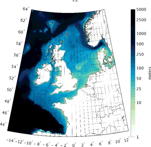
The DCSMv6 is the current operational, 2D storm-surge model that has recently been developed as part of a comprehensive study to improve water level forecasting in Dutch coastal waters. It is developed as an application of the WAQUA software package, which solves the depth-integrated shallow-water equations for hydrodynamic modeling of free-surface flows (Leendertse 1967; Stelling 1984). The model covers the part of the northwest European continental shelf between 15°W to 13°E and 43°N to 64°N. It has a uniform horizontal resolution of 1/40° in east-west direction and 1/60° in north-south direction, which corresponds to a grid cell size of about 1 × 1 nautical mile. Figure 1 shows the model domain and bathymetry.

Figure 1. The DCSMv6 domain and bathymetry.

2.2. Forcing

In modeling the total water levels, the three main forcing terms to be considered are: the tide-generating forcing, the forcing induced by wind and mean sea level pressure variations, and the forcing induced by the depth-averaged horizontal variations in water density (referred to as the “baroclinic forcing”). Like most models, the DCSMv6 uses the Boussinesq approximation and therefore conserves volume and not mass. This implies that it cannot reproduce the net expansion/contraction of the oceans due to heating/cooling (Greatbatch 1994). There are “pragmatic” solutions to include this signal (Mellor and Ezer 1995; Slobbe et al. 2013b). In this study, we added the signal via the water levels prescribed at the open sea boundaries (see Section 2.3 for further details).

2.2.1. Tide-generating forcing

The tide-generating forces account for the components of the tide with a Doodson number ranging from 55,565 to 375,575. Given the size of the model domain, these cannot be neglected; the forces induce water level variations up to 10 cm (Zijl et al. 2013).

2.2.2. Atmospheric wind and mean sea level pressure

Atmospheric wind and mean sea level pressure data were obtained from the publicly available data of the interim reanalysis project ERA-Interim (Dee et al. 2011) provided by the European Centre for Medium-Range Weather Forecasts. ERA-Interim covers the period from January 1, 1979 onward and provides three-hourly grids with a spatial resolution of 0.75° × 0.75°.

The wind and air pressure fields were interpolated to the DCSMv6 grid using the Generic Mapping Tools (GMT) greenspline routine (Wessel 2009) with a tension factor of zero. To account for the differences between on- and offshore wind regimes, we only used the grid cells that are flagged as “sea” in the ERA-Interim land/sea mask. To convert the wind speeds to wind stresses, we used the Charnock drag formulation (Charnock 1955). This formulation includes the so-called Charnock coefficient; a dimensionless bulk parameter depending upon atmospheric conditions and surface wave parameters that determines the grip of the wind on the sea surface. In our simulations, we used the time/space-varying Charnock coefficients that are part of the ERA-Interim output.

2.2.3. Baroclinic forcing

In operational use, the DCSMv6 includes tides and meteorological forcing only; baroclinic processes are ignored. This is a valid simplification for storm surge predictions a few days ahead as the short-term water level variations induced by baroclinic effects are negligible compared to those induced by tides, winds, and atmospheric pressure variations (especially on the continental shelf). In this study, however, we aim to obtain LAT with respect to the (quasi-)geoid. As such, we need to include the baroclinic contribution (see Slobbe et al. 2013a). Therefore, we extended the DCSMv6 to account for depth-averaged horizontal variations in water density using the method described by Slobbe et al. (2013b). A key feature of that methodology is that the depth-averaged horizontal baroclinic pressure gradients are treated as a diagnostic variable in the model simulations.

The pressure gradient fields were computed from temperature and salinity fields obtained from a reanalysis with a 3D hydrodynamic model defined on a larger domain than the DCSMv6. In this study, we used the 3D daily mean temperature and salinity fields from the Atlantic–European North West Shelf–Ocean Physics Reanalysis conducted by the UK Met Office (Wakelin et al. 2016), available at the Copernicus Marine Environment Monitoring Service (http://marine.copernicus.eu/). This reanalysis covers the period January 1985–July 2014 and is based upon the Forecasting Ocean Assimilation Model 7 km Atlantic Margin Model; a hydrodynamic model of the North West European shelf forced at the surface by ERA-interim winds, atmospheric temperature, and precipitation fluxes. The overall procedure to compute the depth-averaged horizontal baroclinic pressure gradients consists of four steps:

Step 1. Transform salinity and temperature to water density. The daily mean salinity and temperature fields exploited in this study are available at 24 geopotential (z-level) vertical levels based upon the standard depths of the International Council for the Exploration of the Sea. To transform them to water density fields, we used the international thermodynamic equation of seawater 2010 (TEOS-10) (IOC, SCOR and IAPSO 2010).

Step 2. Upsample the density profiles. The separation between the vertical levels increases with increasing depth. Using a spline interpolation, we upsampled each density profile such that the maximum sampling interval is 25 m.

Step 3. Compute the depth-averaged horizontal baroclinic pressure gradients. The pressure gradients in x (east–west) and y (north–south) directions, Γ_x and Γ_y, respectively, were computed using (Slobbe et al. 2013b, Eq. 5):(1) Herein, d is the depth below the reference surface, g is the gravity acceleration (assumed to be constant), L is the number of depth layers in the 3D model from which the temperature and salinity fields are derived, j and l are the layer indices, h_j and h_l are the thickness of layers j and l, and ρ_j and ρ_l are the mean water density of layers j and l.

Step 4. Interpolate the depth-averaged horizontal baroclinic pressure gradients to the DCSMv6 grid nodes. The interpolation was conducted using GMT’s surface routine (Wessel and Smith 1995) with a tension factor of zero.

2.3. Open Boundary Conditions

At the open sea boundaries, boundary conditions were defined in the form of water levels. These were composed as the sum of the four main contributors to the total water levels: the astronomical tide, surge, baroclinic, and steric water level variations. To obtain a model that provides water levels with respect to the European Gravimetric Geoid 2015 model (EGG2015) (Denker 2013, 2015) in the mean-tide system (e.g., Mäkinen and Ihde 2008), a constant was added to the prescribed water levels. This constant was computed from the differences between an observation- and model-derived mean dynamic topography surface (Slobbe et al. 2013b).

2.3.1. The astronomical tide

The astronomical tidal water level (ζ_a(ϑ, λ, t)) was derived by a harmonic expansion using 26 constituents (International Hydrographic Organization - Tides, Water Level And Currents Working Group 2016), namely 5 long-term constituents: Ssa, MSf, Mm, Mf, and Mfm; 11 diurnal constituents: 2Q₁, σ₁, Q₁, ρ₁, O₁, χ₁, π₁, P₁, K₁, Φ₁, and θ₁; and 10 semi-diurnal constituents 2N2, μ₂, N₂, ν₂, M₂, λ₂, L₂, T₂, S₂, and K₂(2) where f_iH_i, ω_i, and G_i are the amplitude, angular velocity, and phase of harmonic constituent i, respectively; and (V₀ + u)_i links the local time basis to the orbital positions of the Sun, Moon, and Earth. The amplitudes and phases of the five long-term constituents were taken from the FES2012 tidal atlas (Carrère et al. 2012). The amplitudes and phases of the other constituents are the same as those being used in the operational version of the DCSMv6, see Zijl et al. (2013) for further details. The 18.6-year nodal tide cycle was approximated by the nodal coefficients f_i(t) and u_i(t).

2.3.2. Surge

Water level variations induced by the atmospheric wind and pressure forcing were taken from the “Dynamic Atmospheric Correction” product provided by AVISO (CNES/CNRS-Legos/CLS 2016). This product is based on the Mog2D-G high-resolution barotropic model (Carrère and Lyard 2003) for frequencies less than 20 days and the inverted barometer correction otherwise.

2.3.3. The baroclinic water levels

The baroclinic water levels were computed from the 25-hourly mean water levels that are part of the output of the Atlantic–European North West Shelf–Ocean Physics Reanalysis (kindly provided by John Siddorn) by removing the 25-hourly mean astronomical tidal and surge water levels. Remaining high-frequency tide and surge signals were suppressed by applying a Butterworth filter with a passband frequency of 0.2618 rad/sample, a stopband frequency of 0.4488 rad/sample, a passband ripple of 1 dB, and a stopband attenuation of 40 dB.

2.3.4. The steric water levels

The steric water level variations were computed from 3D temperature and salinity grids from EN4 version 4.1.1 (Good et al. 2013) using the methodology described by Frederikse et al. (2016). The added signal is the average over all grid points inside the entire DCSMv6 domain, the Bay of Biscay, and the west of Portugal.

3. Methodology

In this methodological section, we first introduce the methodology applied to compute LAT using the regional, vertically referenced hydrodynamic model. Second, we describe the data assimilation method used in this study. Finally, we describe how we derived tidal water levels and LAT from tide gauge records.

3.1. Computing LAT

LAT is defined as “the lowest tide level which can be predicted to occur under average meteorological conditions and under any combination of astronomical conditions” (International Hydrographic Organization 2011, Technical Resolution 3/1919). There are multiple ways to interpret what is referred to as “average meteorological conditions,” because part of these is subject to periodic variations. Since the seasonal variations are the most pronounced over the time scales we consider in realizing LAT (i.e., one nodal cycle), Slobbe et al. (2013a) proposed to include the multi-year average monthly mean (i.e., the average seasonal) meteorological variations in realizing LAT. This proposal was adopted by the Hydrographic Service of the Royal Netherlands Navy (NLHS). Now, given a model that produces at a grid time series of tidal plus average seasonal meteorological water levels, we obtained the LAT surface by taking at each grid point the minimum water level.

To include the average seasonal meteorological variations, we forced the hydrodynamic model by astronomical tides and the multi-year average monthly mean wind stress, mean sea level pressure, and depth-averaged horizontal pressure gradients induced by horizontal variations in the water density. These multi-year average monthly mean forcing fields were computed by averaging for each calendar month all available forcing fields over the entire 19-year simulation period (1993–2012). The obtained yearly time series were used for the 19-year model run. To avoid jumps in the transition from month to month, the obtained time series were resampled to three-hourly values (the original temporal resolution of the wind speed and mean sea level pressure data) using a cubic spline interpolator. Here, we assigned the multi-year average monthly means to the mid-epochs of each month. The multi-year average monthly mean surge, baroclinic, and steric contributions to the water levels prescribed at the open sea boundaries were obtained in the same way.

3.2. The Steady-State Kalman Filter

The data assimilation method used in this study is the same as the one used in the Dutch operational storm surge forecasting system. The method is extensively described by Zijl et al. (2015). It is based on the Kalman filter (Kalman 1960), which provides optimal state estimates by sequentially combining model and observations taking into account their associated uncertainties. In particular, we used the computationally efficient ensemble-based steady-state Kalman filter (El Serafy and Mynett 2008) in which an average Kalman gain, computed by an Ensemble Kalman filter (Evensen 2003), is used. The steady-state (i.e., average) Kalman gain was computed in three steps (Zijl et al. 2015):

1.	Run an ensemble Kalman filter over a certain period (here the period is January 1, 2007–July 1, 2007), complete with the forecast-analysis cycles, where all observations are assimilated sequentially in time.
2.	Store the Kalman gains with a certain time interval (here the interval was 3 hours).
3.	Compute the time-averaged Kalman gains. In principle, for stable time-invariant systems the Kalman gain becomes constant if the ensemble is infinitely large. However, in practice, the ensemble size is always limited and the estimate of the error covariance, hence the Kalman gain, suffers from a sampling error. Averaging the Kalman gain over time is necessary to reduce this error. The average gain is used as the steady-state Kalman gain.

The data assimilation was conducted using the open source data assimilation toolbox OpenDA; a generic framework for parameter calibration and data assimilation applications (El Serafy et al. 2007; Van Velzen and Segers 2010).

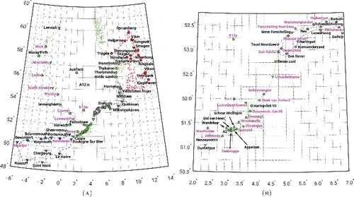
The improvement of the tidal water level modeling obtained with a Kalman filter is to a large extent dependent on the observational network on which one relies. Hence, a careful selection of the observation locations is required. Zijl et al. (2015) discuss a number of items that should be considered. Based on these, they selected 32 tide gauges (both onshore and offshore) of which they assimilated the water levels. In this study, we used the same tide gauges (see Figure 2). We only omitted the use of North Cormorant as there are hardly any data available over the period 1993–2012. This choice of the tide gauge network is optimal for the realization of an LAT surface for the Dutch Continental Shelf. For other areas, the network needs to be selected differently. For instance, in case the area of interest covers the entire North Sea, it is recommended to also include tide gauges in Germany, Denmark, and Norway.

Figure 2. Locations of the tide gauges used in this study. Blue tide gauges are located inside the English Channel, red ones in the Skagerrak–Kattegat, green ones in the North Sea, and gray ones in the Wadden Sea. The tide gauges labeled in magenta belong to the observational network from which tidal water levels are assimilated. A triangular marker means that the tide gauge benchmark was measured using GNNS.

Even though we included the baroclinic forcing in the model, we still applied the bias correction to the assimilated tidal water levels described by Zijl et al. (2015). That is, we replaced the mean water levels by model-derived ones. The latter were obtained from a simulation that had the same setup, but where we did not apply data assimilation. The reason to apply this correction is twofold. First, at some tide gauge locations the model has difficulties in representing the long-term mean water level (Slobbe et al. in press). In particular at the locations where fresh water is discharged, as this forcing is not included in the model. Second, even tiny errors in the vertical referencing of the tide gauges imply large erroneous water fluxes and tilts in the water levels and are a potential source for model instabilities. Numerical experiments (not shown here) confirmed that these instabilities show up, giving rise to large errors in the modeled water levels.

3.3. Preprocessing of the Tide Gauge Data used in the Data Assimilation and Validation

From our internal database, we obtained data from 92 onshore and offshore gauges that include measurements over the time span over which we derived LAT (1993–2012). The locations of these tide gauges are shown in Figure 2. Most tide gauges have a record length covering the entire simulation period, but there are a few exceptions. The Dutch offshore tide gauge A12 has the shortest record; it only starts from February 2009.

The water levels at the tide gauges need to refer to the same reference surface to which the water levels of the hydrodynamic model refer. In this study, this is the EGG2015 in the mean-tide system. Therefore, height transformations were carried out by three different methods. If available, GNSS measurements were used to obtain observed water levels relative to the GRS80 reference ellipsoid after which we subtracted the EGG2015 (applies to all tide gauges indicated with a triangular marker in Figure 2). Else, we added to the observed water levels the difference between either the national (quasi-)geoid height and the EGG2015 (onshore tide gauges) or the DTU13 mean sea surface height (Andersen et al. 2015) and the EGG2015 (offshore tide gauges).

The procedure used to derive LAT from the tide gauge records consist of four steps.

Step 1. Estimate the tidal constituents. The tidal constituents were estimated from the observed water levels by a harmonic analysis. For the Dutch and Belgium tide gauges, we used an available pre-defined set of 95 constituents commonly used in the Netherlands. For the UK tide gauges such a set is also available; it includes 103 constituents. For the remaining tide gauges, we applied the harmonic analysis using both sets. Moreover, we applied an in-house developed software based on the UTide Matlab routines (Codiga 2011) that selects constituents automatically. First, we determined which deep water constituents had a signal-to-noise ratio (SNR) ⩾ 2. From this set, we composed the set of possible shallow water constituents that consist of the found deep water ones. Next, the iterative part of the algorithm begins. In each iteration, we conducted a spectral analysis of the residuals (i.e., the observed water levels minus the tidal water levels obtained from a harmonic synthesis using the constituents selected so far). Per constituent group, we selected the constituent in the set of possible shallow water constituents associated with the largest peak in the spectrum. If the SNR was ⩾ 2, we included the constituent and started the next iteration. The iteration stopped when no more constituents were found.

Step 2. Reconstruct the tidal water levels. The tidal water levels were reconstructed over the entire simulation period with a sampling interval of 10 minutes. In the reconstruction, the amplitude of the solar annual (SA) constituent was set to zero (see step 3 for further details).

Step 3. Add the multi-year average monthly mean water level time series. In all cases, the (final) set of tidal constituents used in the harmonic analysis included the SA constituent. This constituent describes the seasonal variation in water level as a sinusoidal variation with a period of 1 year. To remain consistent with the methodology applied to include the average seasonal meteorological variations into the model (Section 3.1), we followed the same approach here. That is, we first computed the time series of monthly mean water levels. Then we averaged for each calendar month all available mean water levels over our simulation time span. The obtained yearly time series were used for the 19-year model run.

Step 4. Select which tidal water level time series should be used to compute LAT. For the tide gauges not located in the Belgium, Dutch, or UK waters, we obtained three time series with tidal water levels based on three different sets of tidal constituents (step 1). To compute the LAT value to be used in the validation, we used the time series that best fits (in the root-mean-square (RMS) sense) the observed water levels.

This procedure differs from the one suggested in Slobbe et al. (2013a) regarding the treatment of a linear trend in the harmonic analysis. Frederikse et al. (2016) have shown that a linear trend is not an accurate functional model to real long-term sea level variations. Second, we no longer included the average seasonal water level variations via the SA constituent, but applied the same approach used to include these into the model. As noted above, in this way we remain consistent.

4. The Model-Only LAT Realization Versus the Kalman-Filtered LAT Realization

Two LAT realizations were computed. The first is a pure model-derived realization (though the model was calibrated using both tide gauge and radar altimeter data (Zijl et al. 2013)) and is referred to as the “model-only” LAT realization. The second was obtained using the steady-state Kalman filter and is referred to as the “Kalman-filtered” LAT realization. In this section, we first assess the impact of the data assimilation by comparing the two realizations. Next, we validate each realization using LAT values obtained from observed water levels at tide gauges and compare the results. Finally, we compare the Kalman-filtered LAT realization to LAT2013 (Slobbe et al. 2013a).

4.1. The Impact of Data Assimilation

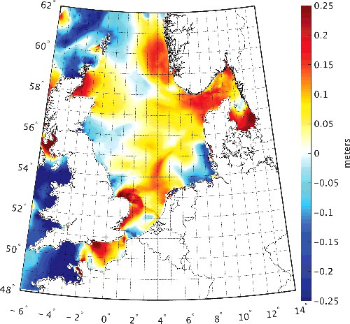
Figure 3 contains two maps; the left map shows the Kalman-filtered LAT realization and the right one the differences between this and the model-only LAT realization. For a brief interpretation and discussion of the LAT signal (Figure 3 a) in the North Sea, we refer to Slobbe et al. (2013a).

Figure 3. LAT relative to the EGG2015 computed using the DCSMv6 over the period January 1993–January 2012 (a). To compute this realization, tidal water levels derived from tide gauge records acquired at 31 locations were assimilated (see Figure 2). Panel (b) shows the difference between the realizations with and without data assimilation.

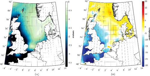
From Figure 3 b, we conclude that the differences between the Kalman-filtered and the model-only LAT realizations can reach several decimeters. They are the largest north of Roscoff and Saint Malo (English Channel) where they reach values up to ∼ 50 cm. In general, their magnitude is large in areas where the LAT signal itself is large. Relative sharp north–south and east–west gradients are observed in the southern North Sea (around 52.5° N, 3° E). There, the differences go from ∼ 5 cm to ∼ −10 cm in both directions. We explain this by the fact that this location coincides with an amphidromic point where the amplitudes are small while the co-phase lines circle around. A similar feature is observed in the English Channel in the vicinity of the degenerate amphidrome off the English coast (around 50.6° N, 2.4° W). Overall, we conclude that the differences have a long wavelength character. A stronger local variability is only observed in the very vicinity of the coastline and in the area of the Norwegian Coastal Current. In the latter case, the tidal variations are “low” anyway (see Figure 3 a) and the differences are only a few centimeters. The observed long-wavelength character of the differences illustrates that the impact of the assimilated tidal water levels is not limited to the coastal waters. This questions the choice made by Turner et al. (2010) to derive the LAT surface beyond 30 km from the coast solely from a satellite altimetry ocean tide model.

4.2. Validation

To assess the quality of the obtained LAT realizations, we compared them to observation-derived LAT values at both onshore and offshore tide gauges. The results are summarized in Figure 4 and Table 1 for the model-only LAT realization, and in Figure 5 and Table 2 for the Kalman-filtered one. Each figure contains four panels. The top panels show a map of the differences between the observation-derived and model-only/Kalman-filtered LAT values (left panel) and the associated histogram (right panel). The maps in the bottom panels show the two contributors to these differences. More particularly, the bottom left map shows the differences between the observation- and model-derived mean sea levels that include the average seasonal variation. These were computed as follows. For both the observation- and model-derived tidal water level time series, we computed the multi-year average monthly mean sea level time series in the same way as we computed the multi-year average monthly mean forcing fields (Section 3.1). Next, we interpolated these time series to the epoch of the LAT event and computed the difference. Note that the epochs of the observation- and model-derived LAT event can differ. Hence, in an extreme case, if one is in summer and the other in winter, the computed difference includes the full range in the seasonal mean sea level variation at the specific location. The bottom right map shows the contribution of the differences between the observation- and model-derived variations of the tidal water level at the epoch of the LAT event. These were computed as the differences between the values shown in the top left panel and the ones in the bottom left panel. The tables present some statistics of the differences between the observation-derived and model-only/ Kalman-filtered LAT values, both for all tide gauges (referred to as “Set A”) and the ones not used in the data assimilation (referred to as “Set B”). Furthermore, the tables contain the statistics per region. Below, we list and discuss the main conclusions drawn from the figures and tables.

Figure 4. Validation of the model-only LAT realization. The top panels show a map of the differences between the observation- and model-derived LAT values (a) and the associated scatterplot (b). The various colors in the histogram refer to the various waters in which the tide gauges are located; the English Channel (blue), the Skagerrak–Kattegat (red), the North Sea (green), and the Wadden Sea (gray). The bottom left map (c) shows the differences between the observation- and model-derived mean sea levels. The bottom right map (d) shows the contribution of the differences between the observation- and model-derived variations of the tidal water level at the epoch of the LAT event. These were computed as the differences between the values shown in panel (a) and panel (c).

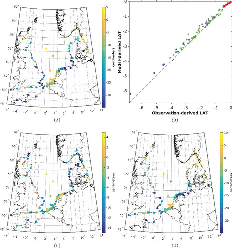
Figure 5. Validation of the Kalman-filtered LAT realization. The top panels show a map of the differences between the observation- and model-derived LAT values (a) and the associated scatterplot (b). The various colors in the histogram refer to the various waters in which the tide gauges are located; the English Channel (blue), the Skagerrak–Kattegat (red), the North Sea (green), and the Wadden Sea (gray). The bottom left map (c) shows the differences between the observation- and model-derived mean sea levels. The bottom right map (d) shows the contribution of the differences between the observation- and model-derived variations of the tidal water level at the epoch of the LAT event. These were computed as the differences between the values shown in panel (a) and panel (c).

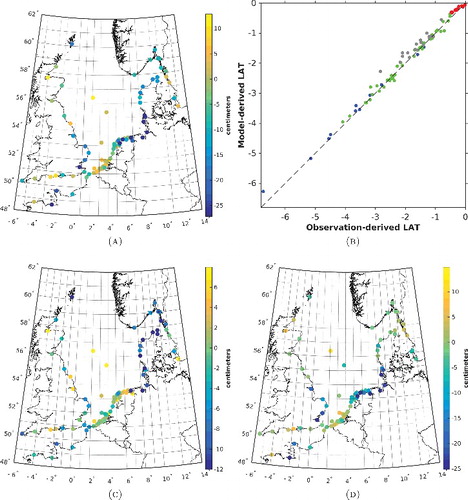
Table 1. Statistics of the differences between the observation- and model-only LAT values shown in Figure 4 a. Set A included all tide gauges, while Set B only included the tide gauges that did not belong to the observational network used in the data assimilation.

Set oftide gauges	Region	Nr.	RMS(cm)	range(cm)	mean(cm)	std(cm)
A	English Channel	12	30.0	52.0	−26.5	14.6
	North Sea	47	15.6	58.3	−10.9	11.3
	Skagerrak–Kattegat	15	9.2	22.8	−6.7	6.6
	Wadden Sea	18	29.1	62.9	−24.6	15.8
	All	92	20.5	79.3	−14.9	14.1
B	English Channel	9	30.8	52.0	−26.5	16.7
	North Sea	23	17.6	58.3	−12.8	12.3
	Skagerrak–Kattegat	15	9.2	22.8	−6.7	6.6
	Wadden Sea	14	32.4	62.9	−28.6	15.6
	All	61	22.8	79.3	−16.9	15.3

Table 2. Statistics of the differences between the observation- and Kalman-filtered LAT values shown in Figure 5 a. Set A included all tide gauges, while Set B only included the tide gauges that did not belong to the observational network used in the data assimilation.

Set oftide gauges	Region	Nr.	RMS(cm)	range(cm)	mean(cm)	std(cm)
y	English Channel	12	16.6	57.1	−7.5	15.5
	North Sea	47	10.8	57.6	−2.4	10.6
	Skagerrak–Kattegat	15	9.5	21.2	−7.2	6.4
	Wadden Sea	18	24.5	59.5	−19.2	15.7
	All	92	15.1	77.6	−7.2	13.4
n	English Channel	9	18.7	57.1	−8.2	17.8
	North Sea	23	13.8	57.6	−5.0	13.1
	Skagerrak–Kattegat	15	9.5	21.2	−7.2	6.4
	Wadden Sea	14	27.7	59.5	−23.4	15.4
	All	61	17.9	77.6	−10.2	14.9

1.	The control data suggest a much better performance of the Kalman-filtered LAT realization compared to the model-only LAT realization. We summarized the agreement with the observation-derived LAT values by the RMS differences. In favor of the Kalman-filtered LAT realization, the RMS value reduced from 20.5 to 15.1 cm (Set A), i.e., a reduction of ∼26%. For Set B, the RMS value reduced by ∼21% (22.8 to 17.9 cm). Note, however, that there are strong regional differences. The largest reduction was observed in the English Channel: ∼45% and ∼39% for Set A and Set B, respectively. For the North Sea the reductions were, respectively, ∼31% and ∼22%. In the Skagerrak–Kattegat, we observed a slight increase (∼3% for both Set A and B).
2.	The higher accuracy of the Kalman-filtered LAT realization is explained by an improved model representation of both the mean sea level and tidal water level variations. Errors in the model representation of LAT relative to the geoid are introduced by errors in the model representation of both the mean sea level and the tidal water level variations. The fact that both errors decreased, can immediately be observed by comparing the bottom panels of Figure 4 to those of Figure 5. The explanation for the improved representation of the mean sea level is twofold. Partly, this reflects an improved representation of the average seasonal mean sea level variations. The representation of the “static” mean sea level (i.e., the mean water level over the entire simulation period) signal did not improve. This cannot even be the case, because as part of the preprocessing we replaced the mean of the observation-derived tidal water levels by the mean of the modeled tidal water levels obtained in the model-only simulation (Section 3.2). The other reason is that discrepancies between the timing of the observation-derived and Kalman-filtered LAT events are lower than the corresponding discrepancies for the model-only LAT realization: ∼ 10.5 days versus ∼ 28 days (computed as the average difference between the days-of-the-year at which the LAT events occurred). Indeed, since we included the average seasonal variation of the mean sea level, any difference in timing of the LAT event gave rise to a signal.
3.	The differences to control data increase in the German Bight and along the Danish coast till Skagen. This behavior is observed for both LAT realizations. By comparing the lower left and right panels in Figures 4 and 5, we conclude that the errors are dominated by errors in the representation of the mean sea level. This makes sense because the further to the north, the smaller the tidal water level variations (see Figure 3 a).
4.	In the English Channel, the differences to control data are the largest on the French side. Again, this behavior is observed for both LAT realizations (though more pronounced for the model-only one). In case of the Kalman-filtered LAT realization, this can be understood by the fact that our observational network did not include any tide gauge on the French side. At the same time, however, we need to mention that the relative discrepancies on both sides of the English Channel are of similar magnitude. The relative discrepancies were obtained by dividing the differences between the observation-derived and model-only/Kalman-filtered LAT values by the observation-derived LAT values themselves.
5.	The presented statistics are significantly impacted by a few large differences to control data. At some tide gauges, the differences between observation-derived and model-only/Kalman-filtered LAT values reach several decimeters. The four largest differences were observed at the Wilhelmshaven, Saint Malo, Wittduen, and Sheerness tide gauges. Because the total number of tide gauges is quite limited, the outlying behavior at these locations significantly impacts the statistics. When we, for example, removed the largest difference between the observation- and Kalman-filtered LAT values, the RMS difference reduced from 15.1 to 14.0 cm for set A and from 17.9 to 16.6 cm for set B. These larger differences may be explained by either model deficiencies or by limitations in the procedure to derive LAT from tide gauge records (see Section 3.3). For instance, Zijl et al. (2013) identified the lack of resolution in the model as responsible for larger differences between observed and modeled water levels at the Sheerness tide gauge. Limitations in the procedure to derive LAT may include (i) the use of a fixed set of tidal constituents for the Belgium, Dutch, and UK tide gauges, and (ii) the use of nodal corrections rather than including the nodal modulation terms into the estimation process. Regarding the latter, the nodal corrections are based on the equilibrium tide and assume a more or less linear response to the forcing from the tidal potential, which is less accurate in shallow water (e.g., Ku et al. 1985). Overcoming both limitations would have required to gain a detailed knowledge of the situation in the vicinity of each tide gauge. This was not achievable in the framework of this study. To assess the impact these limitations have on the observation-derived LAT values at the tide gauges along the coast of the UK, we compared our values to the ones provided by the National Tide and Sea Level Facility (http://www.ntslf.org/tides/hilo). For the Cromer and Sheerness tide gauges, we found differences of 21 cm and 11 cm, respectively. Using the values provided by the National Tide and Sea Level Facility, we obtained smaller differences between the observation-derived and the Kalman-filtered LAT values. The differences at all other tide gauges were smaller (RMS is 5.2 cm).
6.	In Dutch waters, the accuracy of both LAT realizations is higher than the overall statistics suggest. The DCSMv6 is the operational model used in the Netherlands to forecast storm surges. As such, it is particularly designed to show the best performance along the Dutch coast. Illustrative in this respect is the fact that the top five tide gauges where we observed the worst agreement with the observation-derived LAT values are all outside the Dutch waters. Another explanation for the improved accuracy is that 18 out of the 31 Dutch tide gauges were part of the observational network used in the data assimilation. When computing the statistics using only the Dutch tide gauges of Set A, the RMS difference for the Kalman-filtered LAT realization equals 10.5 cm. When we compute the values per region, we obtain 6.6 cm for the North Sea (19 tide gauges) and 14.8 cm for the Wadden Sea (12 tide gauges). For the model-only LAT realization, these values are 13.7 cm (all), 8.0 cm (North Sea), and 19.6 cm (Wadden Sea). To draw more definite conclusions, we recommend to conduct a further validation of the obtained LAT realization by using, e.g., (one of) the methods suggested by Iliffe et al. (2013).

4.3. Comparison to LAT2013

Next, we compare the obtained Kalman-filtered LAT realization to LAT2013 (Slobbe et al. 2013a). The latter realization is currently used operationally by the NLHS. Figure 6 shows a spatial rendition of the differences between the Kalman-filtered LAT realization and LAT2013. Over the Dutch North Sea, the minimum and maximum differences are − 10.8 and 16.5 cm, respectively. The RMS of the differences equals 8.4 cm. In the Wadden Sea and Dutch estuaries, the differences are much larger. In these waters, however, the NLHS concluded that the LAT2013 surface is not accurate.

Figure 6. The Kalman-filtered LAT realization minus LAT2013. LAT2013 was interpolated to the DCSMv6 model grid by a linear interpolation. For points outside the convex hull, a nearest neighbor extrapolation was applied.

Because there are many differences in the experimental setups used to realize the two surfaces (see Table 3 for a summary), we do not attempt to explain the differences observed in Figure 6 in detail. Instead, we validated LAT2013 in the same way as we validated the Kalman-filtered LAT realization to illustrate the better performance of the latter. The results are summarized in Figure 7 and Table 4. To remain consistent, the same validation data set was used. In doing so, we ignored the fact that the two realizations were computed over a different time span (see Table 3). The associated differences, however, are believed to be negligible compared to the other contributors. The inconsistency in the time span is the reason, however, why we cannot create the maps shown in the two bottom panels of Figure 5. Note, that the tide gauges Appelzak, Den Oever, Eemshaven, Kornwerderzand, Klagshamn, and Stenungsund are outside the DCSMv5 computational grid used to compute LAT2013. This causes a small inconsistency between the statistics presented in Tables 2 and 4. Below, we list and discuss our main findings.

Figure 7. Validation of the model-only LAT realization obtained in 2013 (Slobbe et al. 2013a). The panels show a map of the differences between the observation- and model-derived LAT values (a) and the associated scatterplot (b). The various colors in the histogram refer to the various waters in which the tide gauges are located; English Channel (blue), Skagerrak–Kattegat (red), North Sea (green), and Wadden Sea (gray).

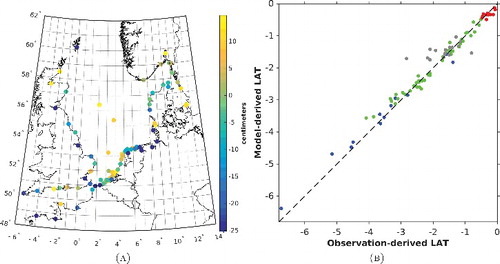
Table 3. Summary of the differences between LAT2013 (Slobbe et al. 2013a) and the Kalman-filtered LAT realization obtained in this study.

	LAT2013	Kalman-filtered LAT
Hydrodynamic model	DCSM version 5	DCSM version 6
Time span	1984–2004	1993–2012
Forcing
internal tides	neglected	included
wind & mean sea	ERA-Interim (1.5° × 1.5°)	ERA-Interim (0.75° × 0.75°)
level pressure
baroclinic	Reanalysis (Holt et al. 2005)	Reanalysis (Wakelin et al. 2016)
	(1/6° × 1/9°, monthly mean)	(1/9° × 1/15°, daily mean)
Open boundary cond.
tides	harmonic analysis, 12 constituents	harmonic analysis, 26 constituents
surge	inverted barometer correction	Dynamic Atmospheric Correction
	(Wunsch and Stammer 1997)	(CNES/CNRS-Legos/CLS 2016)
baroclinic	Reanalysis (Holt et al. 2005)	Reanalysis (Wakelin et al. 2016)
	(1/6° × 1/9°, monthly mean)	(1/9° × 1/15°, daily mean)
steric	Reanalysis (Holt et al. 2005)	EN4 version 4.1.1
	computed using	(Good et al. 2013)
	(Slobbe et al. 2013b, Eq. 2.10)	computed by
		Frederikse et al. (2016)
Data assimilation	no	yes
Vertical reference	EGG2008	EGG2015

Table 4. Statistics of the differences between the observation- and LAT2013 values shown in Figure 7 a. Set A included all tide gauges, while Set B only included the tide gauges that did not belong to the observational network used in the data assimilation.

Set oftide gauges	Region	Nr.	RMS(cm)	range(cm)	mean(cm)	std(cm)
y	English Channel	12	24.2	91.5	−8.7	23.6
	North Sea	46	16.0	81.2	−2.6	16.0
	Skagerrak–Kattegat	13	9.6	32.9	3.8	9.2
	Wadden Sea	15	44.2	185.5	−18.2	41.7
	All	86	24.0	185.5	−5.2	23.5
n	English Channel	9	26.0	91.5	−7.0	26.5
	North Sea	22	19.4	81.2	−4.1	19.4
	Skagerrak–Kattegat	13	9.6	32.9	3.8	9.2
	Wadden Sea	12	49.3	185.5	−23.7	45.1
	All	56	28.3	185.5	−6.9	27.6

1.

The Kalman-filtered LAT realization shows a much better agreement to control data. As before, we used the RMS difference to summarize the agreement with the observation-derived LAT values. In favor of the Kalman-filtered LAT realization, the RMS value reduced from 24.0 to 15.1 cm (Set A), i.e., a reduction of ∼37%. The same percentage was obtained when using Set B (28.3 to 17.9 cm). Again, there are strong regional differences. The largest reduction was observed in the Wadden Sea: ∼45% for both Set A and B. Followed by the North Sea and English Channel (in all cases ∼30%). In the Skagerrak–Kattegat, we did not observe a significant change of the RMS differences.

2.

The differences to control data show stronger local variability in case of LAT2013. Based on a visual comparison of Figure 5 a and Figure 7 a, we conclude that the latter shows more local variability, i.e., more pronounced scatter among tide gauges located close to each other. The main explanation is the increased spatial resolution of the DCSMv6 compared to the DCSMv5; local processes are much better resolved.

5. LAT in Very Shallow Waters

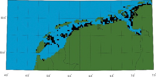
Another main objective of this manuscript concerns the realization of a chart datum in intertidal zones (areas that are above water at low tide and under water at high tide). In our target area, this applies in particular to large parts of the Wadden Sea. Figure 8 shows a map of the Wadden Sea indicating the grid cells that are temporary set dry during low tides. In reality, the intertidal area is even larger (Common Wadden Sea Secretariat 2017). We attribute the differences between the actual intertidal area and its representation by the DCSMv6 to the lack of resolution in the model to represent the complex Wadden Sea bathymetry. The latter is characterized by deep channels and gullies surrounded by shallow intertidal flats. The problem is that LAT is not defined in the intertidal area. Indeed, the minimum tidal water level over one nodal cycle (our operational definition of LAT) is the “no-water” level. The practical consequence of taking the no-water level as chart datum would be that the charted bathymetry becomes zero. The latter makes a bathymetric chart meaningless.

Figure 8. This map of the Dutch Wadden Sea area shows the grid cells that are temporary set dry during low tides (black). Green grid cells are land and blue ones never fall dry.

The most straightforward solution seems to adopt another tidal datum as chart datum or to use the vertical reference surface used on land, i.e., the (quasi-)geoid. Indeed, in this way the problem that the charted bathymetry becomes zeros is avoided. The price to pay is, however, that pilots have to deal with a discontinuity in the charted bathymetry when entering these waters. Not to mention that it will become difficult to keep track on what chart datum is used at a particular location. Note that in the Dutch rivers already two chart datums are in use. For the rivers in which the water levels are determined by the water levels at sea (known as the “Benedenrivierengebied”), an agreed low water level is used that is referred to as “approximately LAT.” Otherwise an agreed low river level is used that corresponds to the water level at the agreed low discharge in Lobith. Introducing a fourth one for the Wadden Sea and estuaries will be a new source of confusion and as such does not support safe navigation.

Here, we propose to use a variant of the engineering approach applied in the realization of the LAT–MSL separation matrix in 2006 (Kwanten 2007). That is, for all grid cells inside the Wadden Sea the separation LAT–geoid is replaced by the separation pseudo LAT–geoid. The latter is obtained in a second model run that equals the one in which the separation LAT–geoid is determined except that all water levels prescribed at the open sea boundaries and the ones assimilated into the model are enlarged by a constant value large enough to prevent that any cell falls dry. By trial and error, we found that 2 m of extra water suffices. Afterward, the pseudo-LAT realization is lowered by this constant. The absolute differences between the obtained pseudo-LAT realization and the Kalman-filtered LAT realization at the Dutch Wadden Sea/North Sea boundary were all below 3.2 cm. In the German Bight and Danish Wadden Sea, these differences increased to max 10.9 cm. Remember that in the German and Danish parts of the Wadden Sea, no tide gauges are located from which data were assimilated. It is the assimilation of tidal water levels that reduced the impact of adding 2 m of waters on the tidal propagation. Without data assimilation, the above outlined approach does not work. So, a direct replacement of the LAT surface in the Dutch Wadden Sea by the pseudo-LAT surface would only introduce a small discontinuity at the boundary. We anyway decided to remove that, by adding a “corrector surface” to the pseudo-LAT surface. This corrector surface was obtained by interpolating the differences between LAT and pseudo-LAT at the Wadden Sea/North Sea boundary to all grid cells in the Wadden Sea using the constraint that they are zero at the shoreline.

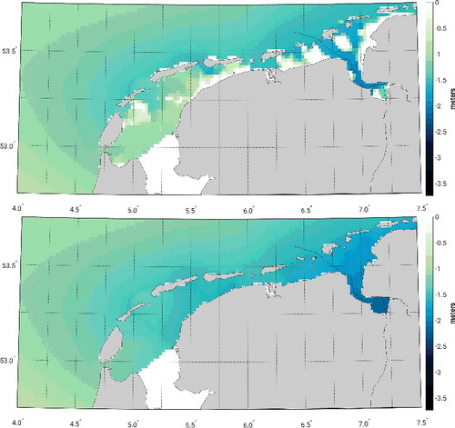
The original Kalman-filtered LAT realization and the combined Kalman-filtered LAT/ pseudo-LAT realization for the Dutch Wadden Sea are shown in Figure 9. Clearly, the latter surface is smoother than the original LAT surface. The price to pay is that it has lost its physical meaning: it might even be below the sea floor.

Figure 9. The Kalman-filtered LAT realization relative to EGG2015 for the Dutch Wadden Sea computed using the DCSMv6 over the period January 1993–January 2012 (a). Panel (b) shows the combined Kalman-filtered LAT/pseudo-LAT realization relative to the EGG2015.

6. Summary, Conclusions, and Recommendations

In this paper, we first presented a novel method to combine a model-derived LAT–geoid surface with observation-derived LAT–geoid values at tide gauges. Whereas all other published methods known to the authors combine observation- and model-derived LAT in a post-processing step, we combine them by assimilating tidal water levels derived from tide gauge records into the model using a steady-state Kalman filter. In doing so, the combination is guided by the model physics and we do not need to rely on questionable assumptions like isotropy or on the properties of the applied interpolator. The obtained “Kalman-filtered LAT realization” was compared to (i) the LAT realization obtained without data assimilation (“the model-only LAT realization”), (ii) observation-derived LAT values at both onshore and offshore tide gauges, and (iii) the LAT2013 realization obtained by Slobbe et al. (2013b).

When validating the Kalman-filtered LAT realization using observation-derived LAT values at tide gauges, we obtained an overall RMS difference of 15.1 cm in case all tide gauges were considered (Set A) and 17.9 cm in case we only considered the tide gauges not used in the data assimilation (Set B). For the North Sea and Wadden Sea, these numbers were 13.8 (Set B) and 27.7 cm (Set B), respectively. Compared to the numbers obtained for the model-only LAT realization, the overall RMS difference reduced by ∼26% for Set A and ∼21% for Set B. However, strong regional differences occur. The largest reduction was observed in the English Channel (∼45% (Set A) and ∼39% (Set B)), while in the Skagerrak–Kattegat we observed a tiny increase of ∼3% for both set A and B. For the North Sea, the reduction was ∼31% (Set A) and ∼22% (Set B). The reduction was attributed to an improved model representation of both the average seasonal mean sea level and tidal water level variations. The presented statistics were shown to be significantly impacted by a few large discrepancies. These were explained by the lack of resolution in DCSMv6 to resolve the local processes in the areas where the large discrepancies showed up, as well as by limitations in the procedure used to derive LAT from the tide gauge records. Moreover, we showed that the accuracy of the LAT realizations is higher in the Dutch waters. When we computed the statistics using only the Dutch tide gauges of Set A, the RMS difference for the Kalman-filtered LAT realization equals 10.5 cm. When we computed the values per region, we obtained 6.6 cm for the North Sea (19 tide gauges) and 14.8 cm for the Wadden Sea (12 tide gauges). These numbers are close/below our target accuracy of 10 cm. We recommend however to conduct a further validation of the obtained LAT realization using the methods suggested by Iliffe et al. (2013).

Second, we addressed the problem of realizing LAT in intertidal waters like the Wadden Sea and Dutch estuaries. In these waters, large areas fall dry during low tide. Consequently, LAT is not defined. We identified the area to which this applies and proposed to replace the LAT in the Wadden Sea by what we refer to as pseudo-LAT. The only difference in deriving pseudo-LAT compared to LAT is that all prescribed water levels at the open sea boundaries and all assimilated tidal water levels are enlarged by a constant value large enough to prevent that any cell fall dry during the simulation. Afterward, this constant is removed from the pseudo-LAT realization. From a user point of view the advantage is that “no” new type of chart datum is introduced and hence there is no discontinuity along the borders of these waters.

We want to conclude with some recommendations for future research:

•	Improve vertical referencing of tide gauges. Our experiments (not shown here) revealed that we lack a realization of a regional height system covering the entire model domain that has sufficient accuracy to serve as a vertical reference of the water levels to be assimilated into the model. For this application, the accuracy requirements are stringent as even small errors imply large water fluxes. Related to this, one needs to make sure that offshore tide gauges become properly connected to this height system.
•	Refine model grid in the Wadden Sea and estuaries. This can be realized either by (i) nesting a high-resolution local model or (ii) using an unstructured mesh.
•	Use baroclinic model. In a future work, also the average baroclinic processes associated with fresh water discharge need to be included in the model. More general, a baroclinic (3D) model needs to be used instead of a modified barotropic (2D) model which accounts for the depth-averaged water density variations. Indeed, it is well known that baroclinic processes affect the tidal propagation and hence LAT. In the current setup, we do not account for these effects.
•	Study feasibility and performance of an alternative approach to realize LAT. Finally, the feasibility and performance of an alternative approach to realize LAT with respect to the geoid needs to be investigated. In this approach, the model-derived LAT is not obtained from modeled tidal water levels but from the reconstructed tidal water levels based on a harmonic analysis applied to model-derived total water levels. In doing so, the approaches to derive the observation- and model-derived LAT values are fully consistent. Numerically, however, the implementation of such an approach imposes great challenges and there is no guarantee that it will improve the accuracy of the LAT realization in an absolute sense. One may argue that from a practical point of view the latter is not needed anyway. If there is a need to obtain a more accurate realization of the chart datum, we doubt whether LAT is the best choice given the intrinsic uncertainty at which we can extract “the tide.” Here, the probabilistic design of chart datum proposed in 2013 (Slobbe et al. 2013b) might be a reasonable alternative. Definitely, this choice allows to realize a unified European depth datum as, contrary to the LAT, it also has a meaning in waters where the tidal variations are small.

Acknowledgments

This study was performed in the framework of the Netherlands Vertical Reference Frame (NEVREF) project, funded by the Netherlands Technology Foundation STW. This support is gratefully acknowledged. In addition the authors gratefully acknowledge the support of the UK Met Office for providing the results of the North West European Shelf Reanalysis. Tide gauge data were kindly provided by the Vlaamse Hydrografie. Agentschap voor Maritieme Dienstverlening en Kust, Afdeling Kust, Belgium; Danish Coastal Authority; Danish Meteorological Institute; Danish Maritime Safety Administration; Service Hydrographique et Océanographique de la Marine, France; Bundesamt für Seeschifffahrt und Hydrographie, Germany; Marine Institute, Ireland; Rijkswaterstaat, Netherlands; Norwegian Hydrographic Service; Swedish Meteorological and Hydrological Institute; and U.K. National Tidal and Sea Level Facility (NTSLF) hosted by POL. We also acknowledge the valuable comments of two anonymous reviewers.

Additional information

Funding

Stichting voor de Technische Wetenschappen (12553).

References

- Andersen, O. B., P. Knudsen, and L. Stenseng. 2015. The DTU13 MSS (Mean Sea Surface) and MDT (Mean Dynamic Topography) from 20 Years of Satellite Altimetry. Berlin, Heidelberg: Springer. pp. 1–10. doi:10.1007/1345_2015_182.
- Carrère, L. and F. Lyard. 2003. Modeling the barotropic response of the global ocean to atmospheric wind and pressure forcing - comparisons with observations. Geophysical Research Letters 30 (6): n/a–n/a. doi:10.1029/2002GL016473.
- Carrère, L., F. Lyard, M. Cancet, L. Roblou, and A. Guillot. 2012. FES2012: A new tidal model taking advantage of nearly 20 years of altimetry measurements. Presented at the Ocean Surface Topography Science Team 2012 Meeting, Venice-Lido, Italy, September 22–29, 2012.
- Charnock, H. Wind stress on a water surface. 1955. Quarterly Journal of the Royal Meteorological Society 81: 639–640. doi: 10.1002/qj.49708135027.
- CNES/CNRS-Legos/CLS. 2016. Dynamic Atmospheric Correction. Available at http://www.aviso.altimetry.fr/en/data/products/auxiliary-products/atmospheric-corrections.html. Last accessed July 2016.
- Codiga, D. L. 2011. Unified tidal analysis and prediction using the UTide Matlab functions. Technical Report, Graduate School of Oceanography, University of Rhode Island, Narragansett, RI. 59 pp.
- Common Wadden Sea Secretariat. 2017. Habitats & Protected Areas. Available at http://www.waddensea-secretariat.org/monitoring-tmap/tmap-results/habitats-protected-areas. Last accessed March 2017).
- Dee, D. P., S. M. Uppala, A. J. Simmons, P. Berrisford, P. Poli, S. Kobayashi, U. Andrae, M. A. Balmaseda, G. Balsamo, P. Bauer, P. Bechtold, A. C. M. Beljaars, L. van de Berg, J. Bidlot, N. Bormann, C. Delsol, R. Dragani, M. Fuentes, A. J. Geer, L. Haimberger, S. B. Healy, H. Hersbach, E. V. Hólm, L. Isaksen, P. Kållberg, M. Köhler, M. Matricardi, A. P. McNally, B. M. Monge-Sanz, J.-J. Morcrette, B.-K. Park, C. Peubey, P. de Rosnay, C. Tavolato, J.-N. Thépaut, and F. Vitart. 2011. The ERA-Interim reanalysis: configuration and performance of the data assimilation system. Quarterly Journal of the Royal Meteorological Society 137 (656): 553–597. doi: 10.1002/qj.828.
- Denker, H. 2013. Regional Gravity Field Modeling: Theory and Practical Results. Sciences of Geodesy - II, G. Xu (ed.), . Berlin Heidelberg: Springer. pp. 185–291. doi: 10.1007/978-3-642-28000-9_5.
- Denker, H. 2015. A new European Gravimetric (Quasi)Geoid EGG2015. 26th IUGG General Assembly, June 22–July 2, Prague, Czech Republic.
- El Serafy, G. Y., H. Gerritsen, S. Hummel, A. H. Weerts, A. E. Mynett, and M. Tanaka. 2007. Application of data assimilation in portable operational forecasting systems—the datools assimilation environment. Ocean Dynamics, 57 (4): 485–499. doi: 10.1007/s10236-007-0124-3.
- El Serafy, G. Y. and A. E. Mynett. 2008. Improving the operational forecasting system of the stratified flow in Osaka Bay using an ensemble Kalman filterbased steady state Kalman filter. Water Resources Research, 44 (6): n/a–n/a. doi: 10.1029/2006WR005412. W06416.
- Evensen, G. 2003. The ensemble Kalman filter: Theoretical formulation and practical implementation. Ocean Dynamics 53 (4): 343–367. doi: 10.1007/s10236-003-0036-9.
- Frederikse, T., R. Riva, D. C. Slobbe, T. Broerse, and M. Verlaan. 2016. Estimating decadal variability in sea level from tide gauge records: An application to the north sea. Journal of Geophysical Research: Oceans 121 (3): 1529–1545. doi: 10.1002/2015JC011174.
- Good, S. A., M. J. Martin, and N. A. Rayner. 2013. En4: Quality controlled ocean temperature and salinity profiles and monthly objective analyses with uncertainty estimates. Journal of Geophysical Research Oceans 118 (12): 6704–6716. doi: 10.1002/2013JC009067.
- Greatbatch, R. J. 1994. A note on the representation of steric sea level in models that conserve volume rather than mass. Journal of Geophysical Research 99: 12767–12771. doi: 10.1029/94JC00847.
- Holt, J. T., J. I. Allen, R. Proctor, and F. Gilbert. 2005. Error quantification of a high-resolution coupled hydrodynamic ecosystem coastal ocean model: Part 1 model overview and assessment of the hydrodynamics. Journal of Marine Systems 57 (1–2): 167–188. doi: 10.1016/j.jmarsys.2005.04.008.
- Iliffe, J. C., M. K. Ziebart, J. F. Turner, A. J. Talbot, and A. P. Lessnoff. 2013. Accuracy of vertical datum surfaces in coastal and offshore zones. Survey Review 45 (331): 254–262. doi: 10.1179/1752270613Y.0000000040.
- International Hydrographic Organization. 2011. Resolutions of the International Hydrographic Organization. Publication M-3, 2nd ed., 2010. Available at http://www.iho.int. Updated to December 2016.
- International Hydrographic Organization - Tides, Water Level And Currents Working Group. 2016. Standard Constituent List. Available at https://www.iho.int/mtg_docs/com_wg/IHOTC/IHOTC_Misc/TWLWG_Constituent_list.pdf. Last accessed 28 July 2016.
- IOC, SCOR and IAPSO. 2010. The International Thermodynamic Equation of Seawater - 2010: Calculation and Use of Thermodynamic Properties. Intergovernmental Oceanographic Commission, Manuals and Guides No. 56, UNESCO (English), 196 pp. Available at http://www.teos-10.org/pubs/TEOS-10_Manual.pdf. Last accessed 29 September 2011.
- Ku, L.-F., D. A. Greenberg, C. J. R. Garrett, and F. W. Dobson. 1985. Nodal modulation of the lunar semidiurnal tide in the Bay of Fundy and Gulf of Maine. Science 230 (4721): 69–71. doi: 10.1126/science.230.4721.69.
- Kwanten, M. C. 2007. Memorie Noordzee reductiematrix 2006 (in Dutch). Ministerie van defensie, Koninklijke Marine, Dienst der Hydrografie.
- Leendertse, J. J. 1967. Aspects of a Computational Model for Long-period Water-Wave Propagation. Rand Corporation for the United States Air Force Project Rand.
- Mäkinen, J. and J. Ihde. 2008. The permanent tide in height systems. Observing Our Changing Earth, volume 133 of International Association of Geodesy Symposia,Sansò, F. and M. G. Sideris (eds.). Berlin Heidelberg: Springer. pp. 81–87.
- Mellor, G. L. and T. Ezer. 1995. Sea level variations induced by heating and cooling: An evaluation of the Boussinesq approximation in ocean models. Journal of Geophysical Research 100 (C10): 20565–20577. doi: 10.1029/95JC02442.
- Robin, C., S. Nudds, P. MacAulay, A. Godin, B. De Lange Boom, and J. Bartlett. 2016. Hydrographic vertical separation surfaces (HyVSEPs) for the tidal waters of Canada. Marine Geodesy 39 (2): 195–222. doi: 10.1080/01490419.2016.1160011.
- Schluter, C. 1993. Tidal modelling within a mangrove environment. 11th Australasian Conference on Coastal and Ocean Engineering: Coastal Engineering a Partnership with Nature. Australia: Institution of Engineers. pp. 725.
- Slobbe, D. C., R. Klees, M. Verlaan, L. L. Dorst, and H. Gerritsen. 2013a. Lowest astronomical tide in the North Sea derived from a vertically referenced shallow water model, and an assessment of its suggested sense of safety. Marine Geodesy 36 (1): 31–71. doi: 10.1080/01490419.2012.743493.
- Slobbe, D. C., R. Klees, M. Verlaan, F. Zijl, B. Alberts, and H. H. Farahani. In press. Height system connection between island and mainland using a hydrodynamic model.
- Slobbe, D. C., M. Verlaan, R. Klees, and H. Gerritsen. 2013b. Obtaining instantaneous water levels relative to a geoid with a 2D storm surge model. Continental Shelf Research 52 (0): 172–189. doi: 10.1016/j.csr.2012.10.002.
- Stelling, G. S. 1984. On the construction of computational methods for shallow water flow problems. PhD Thesis. Delft University of Technology, Delft.
- Turner, J. F., J. C. Iliffe, M. K. Ziebart, C. Wilson, and K. J. Horsburgh. 2010. Interpolation of tidal levels in the coastal zone for the creation of a hydrographic datum. Journal of Atmospheric and Oceanic Technology, 27: 605–613. doi: 10.1175/2009JTECHO645.1.
- Van Velzen, N. and A. J. Segers. 2010. A problem-solving environment for data assimilation in air quality modelling. Environmental Modelling & Software, 25 (3): 277–288. doi: 10.1016/j.envsoft.2009.08.008.
- Wakelin, S., J. While, R. King, E. O’Dea, J. Holt, R. Furner, J. Siddorn, M. Martin, McEwan, R., E. Blockley, and J. Tinker. 2016. Quality Information Document: North West European Shelf Reanalysis NORTHWESTSHELF_REANALYSIS_PHYS_004_009 and NORTHWESTSHELF_REANALYSIS_BIO_004_011. EU Copernicus Marine Service. Issue 3.0.
- Wessel, P. 2009. A general-purpose Green’s function-based interpolator. Computers and Geosciences 35: 1247–1254.
- Wessel, P. and W. H. F. Smith. 1995. New version of the generic mapping tools. EOS Transactions 76: 329–329. doi: 10.1029/95EO00198.
- Wunsch, C. and D. Stammer. 1997. Atmospheric loading and the oceanic “inverted barometer” effect. Reviews of Geophysics, 35: 79–107. doi: 10.1029/96RG03037.
- Zijl, F., J. Sumihar, and M. Verlaan. 2015. Application of data assimilation for improved operational water level forecasting on the northwest european shelf and north sea. Ocean Dynamics 65 (12): 1699–1716. doi: 10.1007/s10236-015-0898-7.
- Zijl, F., M. Verlaan, and H. Gerritsen. 2013. Improved water-level forecasting for the northwest European shelf and north sea through direct modelling of tide, surge and non-linear interaction. Ocean Dynamics 63 (7): 823–847. doi: 10.1007/s10236-013-0624-2.