Validating Geoid Models with Marine GNSS Measurements, Sea Surface Models, and Additional Gravity Observations in the Gulf of Finland

Abstract

Traditionally, geoid models have been validated using GNSS-levelling benchmarks on land only. As such benchmarks cannot be established offshore, marine areas of geoid models must be evaluated in a different way. In this research, we present a marine GNSS/gravity campaign where existing geoid models were validated at sea areas by GNSS measurements in combination with sea surface models. Additionally, a new geoid model, calculated using the newly collected marine gravity data, was validated. The campaign was carried out with the marine geology research catamaran Geomari (operated by the Geological Survey of Finland), which sailed back and forth the eastern part of the Finnish territorial waters of the Gulf of Finland during the early summer of 2018. From the GNSS and sea surface data we were able to obtain geoid heights at sea areas with an accuracy of a few centimetres. When the GNSS derived geoid heights are compared with geoid heights from the geoid models differences between the respective models are seen in the most eastern and southern parts of the campaign area. The new gravity data changed the geoid model heights by up to 15 cm in areas of sparse/non-existing gravity data.

Keywords:

• Dynamic topography
• marine GNSS
• marine gravity
• quasi-geoid
• tide gauge

Introduction

Heights are typically measured as vertical distances to the geoid as zero-level elevation surface. In theory, the geoid coincides with the surface of a homogeneous ocean effected only by gravitation and Earth rotation, i.e., under the absence of external forces such as winds, tides, etc. In case of satellite-based measurement techniques, e.g., GNSS, the height component is relative to a geocentric reference ellipsoid, which is a mathematical idealized representation of the physical Earth. These ellipsoidal heights do not have a connection to the physical Earth, and thus do not contain any information about the direction of water flow. To be able to obtain orthometric or normal heights with GNSS, the observations must be corrected by geoid or quasigeoid heights.

In the EU co-funded project, Finalising Surveys for the Baltic Motorways of the Seas (FAMOS 2020), one goal was to improve the geoid model for the Baltic Sea. This geoid model will serve as the reference surface in the realization of the Baltic Sea Chart Datum 2000 (BSCD2000), a common vertical datum that is currently being introduced for the Baltic Sea (Baltic Sea Hydrographic Commission 2020). The BSCD2000 is based on the definitions for the European Vertical Reference System (EVRS) at land uplift epoch 2000.0 and as such it agrees with the national height systems on land in the surrounding countries, such as the N2000 in Finland and the EH2000 in Estonia. The aim of the FAMOS project is a geoid model with an accuracy of 5 centimeters, and part of the project was to validate the geoid model at sea.

Traditionally, geoid models have been validated with GNSS-levelling benchmarks (precise levelling and GNSS) on land only. As such benchmarks cannot be established offshore, marine areas of geoid models must be evaluated in a different way. In recent years, several shipborne GNSS/gravity campaigns have proven to be successful in complementing and assessing geoid models at sea areas in the Baltic Sea (Varbla et al. 2017, Varbla, Ellmann, and Delpeche-Ellmann 2020; Nordman et al. 2018; Ince et al. 2020) and the Mediterranean Sea (Lavrov et al. 2017).

In 2018, a dedicated GNSS/gravity campaign took place in the eastern part of the Gulf of Finland. The previously available gravity data in the area is sparse or non-existent, causing a large uncertainty in geoid models for the area. In this study we apply the method described in Nordman et al. (2018), where the GNSS-IMU observations are used together with sea surface models (tide gauge surfaces and physical forecast models) in validating already existing geoid models for the area. Additionally, a new geoid model is calculated using the marine gravity data of the present campaign and the new model is also validated.

In “Study area, initialization and data acquisition” we describe the measurement campaign. “From ellipsoidal heights to geoid heights” describes the process to obtain the geoid heights from the GNSS-IMU observations. In “Validating the geoid models” we validate the geoid heights from selected geoid models. Conclusions are given in “Conclusions.”

Study area, initialization and data acquisition

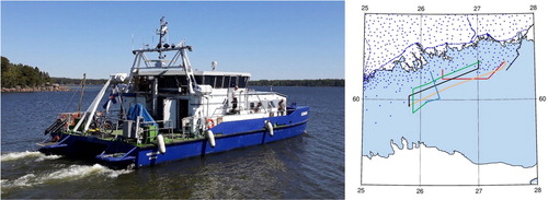
In the early summer of 2018, a dedicated GNSS/gravity campaign was conducted with the marine geology research catamaran, Geomari (Figure 1, left), operated by the Geological Survey of Finland. The Geomari campaign took place in the eastern part of the Finnish territorial waters in the Gulf of Finland, where a gap in our gravity data existed, as gravity measurements have traditionally been taken as single observations on islands, islets, seafloor and sea ice (see the blue dots in Figure 1, right). The right-hand side of the Figure 1 also presents the daily trajectory lines of the Geomari from 21–25.5.2018: Monday (red), Tuesday (orange), Wednesday (black), Thursday (green) and Friday (blue).

Figure 1. The Geomari catamaran at the start of the campaign and the daily trajectory lines: Monday (red), Tuesday (orange), Wednesday (black), Thursday (green) and Friday (blue). Blue dots are the gravity data already existing within the Finnish borders.

Source: Author

During the Geomari campaign the raw GNSS measurements were observed with three geodetic grade GNSS multi frequency antennas: one at the centre of the catamaran, one on starboard side and one on port side of the catamaran. The central antenna was connected to a Novatel dual frequency geodetic receiver and an inertial measurement unit (IMU) to record the movements (pitch, roll, yaw, heave etc.) of the catamaran that are caused by the prevailing heave of the sea. The side antennas were connected to Septentrio GNSS receivers.

In addition, a marine gravimeter was installed on the cabin floor for gravity observations along the tracks. The installation and operation of the gravimeter was conducted by colleagues from the Swedish mapping, cadastral and land registration authority – Lantmäteriet. The exact positions of the instruments were measured in an internal coordinate system of the catamaran.

The catamaran went into a different harbour every night and data was recorded only in daytime during the catamaran’s operation. All the instruments were online for 30 minutes before and after docking/undocking for initialization, especially important for the IMU system. Draft readings were collected at the start and end of each day to estimate the static draft of the catamaran. This was done by measuring the perpendicular distance from the water level to the top of the bollards that are situated at each corner of the catamaran. The vertical locations on top of the bollards were measured beforehand with respect to the vessel’s internal coordinate system.

From ellipsoidal heights to geoid heights

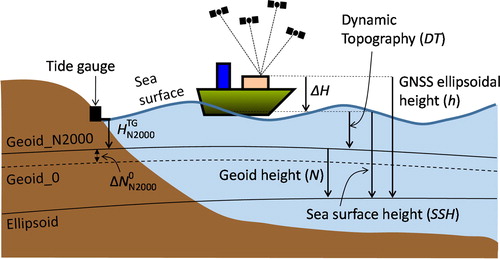
In order to obtain geoid heights, N, from GNSS, the ellipsoidal heights, h, must be reduced first with precise tie measurements, ΔH, to the sea level at the exact measurement time, resulting in sea surface heights (SSH). Next, the prevalent sea surface topography, known as dynamic topography (DT), is modeled and removed from the SSH in the first step. The resulting geoid heights give the distance between the mathematical ellipsoid and the physical geoid surface. Relations between the reference heights and the surfaces are presented in Figure 2, where Geoid_0 is the geopotential surface of a geoid when it is not fitted to a national height system. Geoid_N2000 is the geopotential surface of a geoid aligned to the N2000 height system. ${\Delta N}_{N2000}^0$ is the offset between the aligned and non-aligned geoid models and ${\mathrm{H}}_{N2000}^{TG}$ is the sea level measured by a tide gauge in the N2000 height system.

Figure 2. Relations between the different heights and surfaces. Geoid_0 is the geopotential surface of a geoid when it is not fitted to a national height system. Geoid_N2000 is the geopotential surface of a geoid aligned to the N2000 height system. ${\mathit{\Delta }\mathit{N}}_{\mathit{N}2000}^0$ is the offset between the aligned and non-aligned geoid models and ${\mathrm{H}}_{\mathit{N}2000}^{\mathit{TG}}$ is the sea level measured by a tide gauge in the N2000 height system.

First, in “GNSS base stations and post-processing of the GNSS-IMU” a common set of reference coordinates was calculated for the reference GNSS stations, followed by the post-processing of the GNSS-IMU data. In “From the IMU to the sea surface,” the ellipsoidal heights of the IMU sensor are reduced to the sea surface. Then, to obtain geoid heights, the DT is modelled and removed from the heights at the sea surface in “From the sea surface to the geoid.” Finally, in “Geoid models and coordinate transformations,” the coordinates of the GNSS derived geoid heights are transformed to the reference frames of the selected geoid models. The resulting geoid heights, in desired reference frames, are used for validating the previously existing and the new geoid models.

GNSS base stations and post-processing of the GNSS-IMU

Post-Processing of the collected GNSS data, required GNSS base stations with known coordinates as a reference. From Finland, the stations from the FinnRef (Koivula et al. 2012) and Trimnet (Geotrim 2020) networks were used, and from Estonia the ESTPOS (Metsar, Kollo, and Ellmann 2018) network was employed. FinnRef is the reference network of the Finnish coordinate system operated by the National Land Survey of Finland (NLS), while Trimnet is a private network operated by GeoTrim Oy. ESTPOS is the reference network of the Estonian reference system operated by the Estonian Land Board (Maa-amet). All stations were collecting GNSS data with 1 Hz observing interval throughout the campaign. To ensure a homogenous set of reference coordinates for the base stations, the reference coordinates were calculated in a combined adjustment.

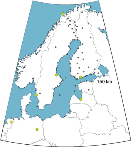
The coordinates of the reference stations, in the IGS14 reference frame, were combined from the daily solutions of the FGI GNSS Analysis Centre between April 26^th and May 12^th (middle epoch 2018.34110), just before the present Geomari campaign. The used procedure followed the guidelines of the Nordic-Baltic NKG GNSS analysis center (Lahtinen et al. 2018). The full network and the reference stations are shown in Figure 3. The daily data was processed using the L3 ionosphere free linear combination, 30 sec sampling interval and 3-degree cut-off angle. The troposphere was modelled using the Global Mapping Function (GMF). The daily solutions were stacked into a combined solution by using minimum constraints on translations over the reference station coordinates.

Figure 3. Reference stations (green circles) and the estimated stations (black dots).

Source: Author

Post-processing of the GNSS-IMU data was done with the Inertial Explorer 8.60 software (NovAtel 2014). The calculation process is called “tightly coupled,” when the differential GNSS method is processed in both directions (forward and reverse) together with the IMU observations. As the GNSS observations refer to the antenna reference point (ARP), which is at the bottom of the antenna base (NovAtel), one must provide the vector (lever arm offset) between the ARP and the sensor of the IMU. Together with the selected base stations the trajectory coordinates of the catamaran were calculated, resulting in coordinates in the IGS14 frame at epoch 2018.34110.

From the IMU to the sea surface

For reducing the ellipsoidal heights to the sea level, the following factors were taken into account:

• Heave movements of the catamaran – derived from the IMU data

• Pitch and roll corrections – derived from the IMU data

• Static draft of the catamaran – obtained from the draft readings

• Dynamic draft, squat effect, of the catamaran – caused by the vessel’s speed.

The Geomari is a catamaran and operated at a steady speed of 5 knots. The sea was calm during the campaign, except for the Thursday. As a result, the effect of the heave was up to 3 cm, although mostly below 1 cm. Additionally, the effects of roll and pitch were extremely small, being most of the time below 1 mm, while in the study of Nordman et al. (2018) these effects were significant at 4 and 11 cm. The static draft readings indicated that the distance between the IMU and the sea level varied between 2.46 and 2.48 m for the whole week. With a steady slow speed, during a calm sea, the movements and changes to the attitude of the vessel proved to be minimal on a research catamaran such as the Geomari.

The squat effect is the hydrodynamic phenomenon, where a moving vessel creates an area of lowered pressure that causes the ship to be closer to the seabed. The effect is approximately proportional to the square of the speed of the vessel. As the Geomari had no predetermined squat table, an attempt was made to estimate it from the decelerations and accelerations of the catamaran. However, the amount of deceleration and acceleration events were few, thus it was difficult to get a reliable estimate. The estimated squat value varied between 2 and 4 cm, which seemed too large (Alvi, personal communication 2018). Instead, we chose to use the squat calculation method by Barrass (2004). According to this method the squat value can be calculated as follows for a vessel in open waters: (1) $$\text{Squat}=\frac{C_b\times V^{2.08}}{30}{\left(\frac{B\times T}{H\times B(7.7+20{\left(1-C_b\right)}^2)-B\times T}\right)}^{2/3},$$(1) where C_b is the block coefficient that describes the shape of the vessel in the water, with a value of 1 being a rectangular block. V represents the speed, B the width and T the mean static draught of the vessel. H is the depth of the water. Using equation 1(1) $$\text{Squat}=\frac{C_b\times V^{2.08}}{30}{\left(\frac{B\times T}{H\times B(7.7+20{\left(1-C_b\right)}^2)-B\times T}\right)}^{2/3},$$(1) , a squat value for the Geomari at a steady speed of 5 knots was estimated to be 0.1–0.4 cm depending on the depth of the sea.

From the sea surface to the geoid

To reduce the heights from the instant sea level to the geoid surface, the effect of the dynamic topography, DT, had to be removed. The DT was modeled using two different methods: tide gauge (TG) and physical model (PM), as described in Nordman et al. (2018).

In the TG method, the instantaneous sea level heights are recorded at coastal TG stations (stars in Figure 4) and given as hourly values. The Finnish TGs refer to the N2000 height system and the Estonian TGs to the EH2000, which are both realizations of the EVRS at land uplift epoch 2000.0 and heights given in these systems are therefore comparable. The TG heights were interpolated to hourly surfaces (Figure 5, bottom right) using thin plate spline regression. The DT at each epoch of the GNSS observations was then estimated from these surfaces using the nearest neighbor method in space and time.

Figure 4. The tide gauges (stars) from Finland and Estonia that were used to model the DT in the Gulf of Finland.

Source: Author

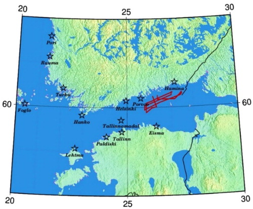
Figure 5. An example of the steps in the process from the original PM surface (top left) to the corrected PM surface (bottom left). The original PM is not aligned to a geodetic height reference and is corrected with a correction surface (top right), calculated from the differences to the tide gauge surface (bottom right). Black dots are the tide gauges.

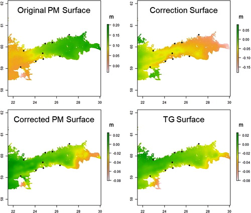
In the PM method, the sea level elevation data of the Baltic Sea physics analysis and forecast model was used (CMEMS 2016). The PM is not aligned to geodetic height reference, as the zero level refers to an arbitrary model zero. Therefore, the PM needs to be aligned to the height reference N2000/EH2000. In Figure 5 the construction of the aligned PM is presented for an epoch in the middle of the campaign. First, the PM is adjusted to the tide gauge readings by using sea level elevation data from the original PM at points close to the tide gauges and creating an hourly surface as in the TG method. Next, the interpolated PM surface is subtracted from the TG surface, resulting in a correction surface (top right). Finally, the correction surface is added to the original PM surface (top left), resulting in a corrected PM surface (bottom left) that is now aligned in N2000/EH2000. Doing this for every epoch, hourly PM surfaces were created and the DT were thereafter estimated in the same way as in the TG method.

Geoid models and coordinate transformations

Four geoid models were used for the comparisons:

• The present Finnish geoid model FIN2005N00 (Bilker-Koivula 2010)

• The Nordic-Baltic geoid model NKG2015 (Ågren et al. 2016)

• The high-resolution Finnish geoid model, FIN_EIGEN-6C4, (Saari and Bilker-Koivula 2018).

• The high-resolution Finnish geoid model, FIN_EIGEN-6C4_GEO, calculated in this study

The Finnish national geoid model, FIN2005N00, was produced by fitting the NKG2004 geoid model to Finnish GNSS/levelling data and as such it is aligned to the N2000 height system (Bilker-Koivula 2010). The Nordic-Baltic gravimetric geoid model, NKG2015, was before release adjusted with an offset of −0.4874 m to fit on average to the GNSS/levelling data of the whole Nordic and Baltic area. It still has a small offset of 2 cm to the N2000 height system (Saari and Bilker-Koivula 2018). The FIN_EIGEN-6C4 and FIN_EIGEN-6C4_GEO models are pure gravimetric geoid models that were not fitted to GNSS/levelling data and therefore still have an offset of 30.4 cm with respect to the N2000 height system (Saari and Bilker-Koivula 2018).

The fourth model is a new version of the FIN_EIGEN-6C4 that was calculated to see the effect of the new gravity data from the Geomari campaign on the geoid model. The new geoid model, FIN_EIGEN-6C4_GEO, is identical to the previous model in every other way except for the inclusion of the gravity data from the Geomari campaign in the geoid calculations.

As the trajectory coordinates refer to the IGS14 reference frame, at epoch 2018.34110 (see “GNSS base stations and post-processing of the GNSS-IMU”), it differs from the coordinate reference frames that are related to the geoid models used in the comparisons. The Finnish national geoid model, FIN2005N00 (Bilker-Koivula 2010), is related to the ETRF96 reference frame at epoch 1997.0. The Nordic geoid model, NKG2015 (Ågren et al. 2016), and the high-resolution Finnish model, FIN_EIGEN-6C4 (Saari and Bilker-Koivula 2018), are related to the ETRF2000 reference frame at epoch 2000.0. Thus, the trajectory coordinates must be transformed to these reference frames for comparisons with the geoid models.

Typically, intra-plate deformations are not taken into account in coordinate transformations between reference frames. However, in the Fennoscandian area glacial isostatic adjustment (GIA) causes movements of up to +1 cm/year in vertical and a few millimetres in horizontal direction. In the area of the Geomari campaign the land uplift varies between 2–4 mm/year, thus the land uplift must be taken into account to obtain cm accuracy. The coordinates were transformed from the IGS14(2018.34110) into ETRF96(1997.0) and ETRF2000(2000.0) according to the method in Häkli et al. (2016) that uses the common Nordic deformation model NKG_RF03vel for applying the intraplate corrections.

Validating the geoid models

Using the TG and PM surfaces, the ellipsoidal heights for the sea surface, the SSH, were reduced to corresponding geoid heights in ETRF96 and ETRF2000. The GNSS derived geoid heights, N_GNSS, were compared with the geoid heights obtained from the geoid models, N_Geoid. In theory, the difference should be zero, but in practice a residual geoid height difference, dN, remains: (2) $$dN=N_{\mathrm{GNSS}}-N_{\mathrm{Geoid}}$$(2)

Finally, averages and standard deviations were calculated from the remaining differences. Detailed daily comparisons of geoid heights derived from the Geomari campaign and geoid heights from the geoid models, described in “Geoid models and coordinate transformations,” are given in Table 1.

Table 1. Statistics of the differences between geoid heights derived from the Geomari GNSS observations and geoid heights from the geoid models FIN2005N00, NKG2015, FIN_EIGEN-6C4 and FIN_EIGEN-6C4_GEO, with DT corrections from the TG (left) and PM (right).

DOY 141 – 145	TG – Tide Gauges (cm)								PM – Physical Model (cm)
	FIN2005 N00		NKG 2015		FIN_EIGEN-6C4		FIN_EIGEN-6C4_GEO		FIN2005 N00		NKG 2015		FIN_EIGEN-6C4		FIN_EIGEN-6C4_GEO
	Avg.	Std.	Avg.	Std.	Avg.	Std.	Avg.	Std.	Avg.	Std.	Avg.	Std.	Avg.	Std.	Avg.	Std.
Mon	5.2	4.1	15.6	4.6	34.4	1.8	41.3	2.1	4.6	4.1	15.0	4.6	33.8	1.8	40.7	2.0
Tue	−3.8	5.7	6.3	6.7	27.0	3.6	34.1	3.6	−4.9	5.7	5.2	6.8	25.9	3.6	33.1	3.7
Wed	3.4	3.1	11.6	3.6	35.1	3.7	43.3	3.3	2.9	3.1	11.2	3.8	34.7	3.5	42.9	3.3
Thu	7.4	4.3	14.3	4.7	39.7	4.1	47.1	4.5	7.5	4.7	14.5	5.2	39.8	4.5	47.2	5.0
Fri	−5.1	3.7	4.5	4.6	28.5	3.7	38.1	3.1	−5.6	3.5	4.1	4.2	28.0	3.4	37.6	2.8
All	2.4	6.4	11.2	6.4	33.8	5.9	41.4	5.9	2.0	6.7	10.8	6.7	33.3	6.3	41.0	6.4

In Table 1 the average of all (Mon–Fri) geoid height differences deviate a lot, from 2.4 cm (FIN2005N00) to 41.4 cm (FIN_EIGEN-6C4_GEO). Taking the geoid height differences as such is causing problems related to the way the geoid models were treated before their release (see “Geoid models and coordinate transformations”). To be able to compare the results obtained with the different models, an offset, the overall average dN value, was removed from each dataset and we analyze the deviations from the average in Table 2.

Table 2. Statistics of the differences, after the removal of the average of the whole campaign, between geoid heights derived from the Geomari GNSS observations with DT corrections from the TG (left) and PM (right) and geoid heights from the geoid models FIN2005N00, NKG2015, FIN_EIGEN-6C4 and FIN_EIGEN-6C4_GEO.

DOY 141 – 145	TG – Tide Gauges (cm)								PM – Physical Model (cm)
	FIN2005 N00		NKG 2015		FIN_ EIGEN-6C4		FIN_ EIGEN-6C4_GEO		FIN2005 N00		NKG 2015		FIN_ EIGEN-6C4		FIN_ EIGEN-6C4_GEO
	Avg.	Std.	Avg.	Std.	Avg.	Std.	Avg.	Std.	Avg.	Std.	Avg.	Std.	Avg.	Std.	Avg.	Std.
Mon	2.8	4.1	4.4	4.6	0.6	1.8	−0.1	2.1	2.6	4.1	4.2	4.6	0.5	1.8	−0.3	2.0
Tue	−6.2	5.7	−4.9	6.7	−6.8	3.6	−7.3	3.6	−6.9	5.7	−5.6	6.8	−7.4	3.6	−7.9	3.7
Wed	1.0	3.1	0.4	3.6	1.3	3.7	1.9	3.3	0.9	3.1	0.4	3.8	1.4	3.5	1.9	3.3
Thu	5.0	4.3	3.1	4.7	5.9	4.1	5.7	4.5	5.5	4.7	3.7	5.2	6.5	4.5	6.2	5.0
Fri	−7.5	3.7	−6.7	4.6	−5.3	3.7	−3.3	3.1	−7.6	3.5	−6.7	4.2	−5.3	3.4	−3.4	2.8
All	0.0	6.4	0.0	6.4	0.0	5.9	0.0	5.9	0.0	6.7	0.0	6.7	0.0	6.3	0.0	6.4

After the removal of the average for the whole campaign in Table 2, the average daily values of the respective geoid models agree better with each other. For example, the difference between the averages for Monday is between −0.1 cm (FIN_EIGEN-6C4_GEO) and 4.4 cm (NKG2015) with TG method, as before the removal of the offset the difference was between 5.2 cm (FIN2005N00) and 41.3 cm (FIN_EIGEN-6C4_GEO). The daily standard deviations of the geoid height differences (Table 2) vary between 1.8 and 6.8 cm during the whole campaign. The variation is dependent on the geoid model used in the comparisons, as the results include the uncertainties of the geoid models. The smallest standard deviations are achieved with the FIN_EIGEN-6C4 and FIN_EIGEN-6C4_GEO models, where the daily variations with the TG method are between 1.8–4.1 cm and between 2.1 and 4.5 cm, respectively. With the FIN2005N00 and NKG2015 the daily variations with the TG method are between 3.1 and 5.7 cm and between 3.6 and 6.7 cm, respectively. During the campaign the sea was the calmest on Wednesday, which is also visible in Table 2, as the standard deviations for all geoid models vary from 3.1 to 3.7 cm within a range of only 0.6 cm (TG) and a corresponding range of 0.7 cm (PM).

The largest daily differences between the geoid models are seen for Monday and Tuesday, where the standard deviations differ up to 2.8 cm (TG and PM, between FIN_EIGEN-6C4 and NKG2015) for Monday, and 3.2 cm (PM, between FIN_EIGEN-6C4 and NKG2015) for Tuesday. During these days the catamaran sailed to the most eastern part of the Finnish territorial waters (Figure 1, red and orange tracks), close to the Russian border. The difference can be explained by the gravity data used to calculate the respective models. The NKG2004 gravimetric geoid model, from which the FIN2005N00 is derived, and the NKG2015 model use different input gravity data for the eastern part of the Gulf of Finland. The FIN_EIGEN models include mostly the same data as the NKG2015, but different data for Russia and the eastern part of the Gulf of Finland (Saari and Bilker-Koivula 2018).

When comparing the standard deviations for the whole campaign, the FIN_EIGEN models fit the best to the GNSS derived geoid heights with an agreement of 5.9 cm (TG) and 6.3 cm (PM) for the FIN_EIGEN-6C4, and 5.9 cm (TG) and 6.4 cm (PM) for the FIN_EIGEN-6C4_GEO. The overall standard deviations of the FIN2005N00 model (TG 6.4 cm, PM 6.7 cm) agreed with those of the NKG2015 model (TG 6.4 cm, PM 6.7 cm). The differences between the TG and PM methods are small, with TG performing slightly better. The TG surface is fitted with a smooth spline function and does not account for small scale variations in the middle of the basin, whereas the physical model should show these better. Thus, we would expect the PM to give better results, but as our measurements are done quite close to the shore it looks like TG is giving more consistent results.

In a final step, we wanted to see if there is any tilt present in the geoid height differences. In order to remove a possible tilt, a first order polynomial was fitted through the comparison differences of the whole campaign and then removed from the differences. The results are given in Table 3.

Table 3. Statistics of the differences, after the removal of offset and tilt for the whole campaign, between geoid heights derived from the Geomari GNSS observations and geoid heights from the geoid models FIN2005N00, NKG2015, FIN_EIGEN-6C4 and FIN_EIGEN-6C4_GEO, with DT corrections from the TG (left) and PM (right).

DOY 141 – 145	TG – Tide Gauges (cm)								PM – Physical Model (cm)
	FIN2005 N00		NKG 2015		FIN_ EIGEN-6C4		FIN_ EIGEN-6C4_GEO		FIN2005 N00		NKG 2015		FIN_ EIGEN-6C4		FIN_ EIGEN-6C4_GEO
	Avg.	Std.	Avg.	Std.	Avg.	Std.	Avg.	Std.	Avg.	Std.	Avg.	Std.	Avg.	Std.	Avg.	Std.
Mon	6.9	3.2	2.5	3.4	2.4	2.4	2.7	2.8	6.3	3.3	2.0	3.4	1.9	2.4	2.0	2.7
Tue	2.3	6.3	−2.2	3.9	−2.1	3.1	−2.2	3.6	2.3	6.3	−3.1	3.9	−3.0	3.1	−3.1	3.7
Wed	8.7	1.7	−1.1	4.0	−1.3	4.1	−1.1	4.0	8.1	1.7	−1.5	4.2	−1.6	3.9	−1.5	4.0
Thu	10.0	3.0	1.1	3.1	1.3	2.9	1.0	3.2	9.9	3.3	1.3	3.5	1.5	3.7	1.2	3.6
Fri	−0.7	1.4	−0.4	3.6	−0.4	3.6	−0.5	2.7	−1.3	1.2	−0.7	3.3	−0.9	3.3	−1.0	2.4
All	0.0	3.7	0.0	4.0	0.0	3.7	0.0	3.8	0.0	4.1	0.0	4.3	0.0	4.0	0.0	4.2

After the removal of offset and tilt the daily standard deviations of the geoid height differences (Table 3) between the GNSS observations and geoid models vary between 1.2 and 6.3 cm during the whole campaign. The daily geoid height differences are more unanimous between the geoid models, especially for the Monday where the standard deviations are between 2.4 and 3.4 cm (TG and PM), whereas before the removal these ranged from 1.8 to 4.6 cm (TG and PM). Additionally, the NKG2015 model now agrees well with the FIN_EIGEN models, as the standard deviations of all data agree with each other within 1 cm.

The smallest standard deviations are achieved with the FIN_EIGEN models, where the daily standard deviations vary between 2.4–4.1 cm (TG) and 2.4–4.0 cm (PM). Overall, the differences between the FIN_EIGEN models are small. However, differences are seen on Monday (TG 0.4 cm, PM 0.3 cm), Tuesday (TG 0.5 cm, PM 0.6 cm) and Friday (TG/PM 0.9 cm). Largest differences are seen on the most eastern and southern tracks (Mon, Tue, Fri), where the gravity measurements were previously sparse or non-existent. The daily standard deviations for the FIN2005N00 and NKG2015 models vary between 1.2–6.3 cm and 3.1–4.2, respectively.

When comparing the standard deviations for the whole campaign, the results are more uniform than before the removal of the tilt. The FIN_EIGEN models agree to the GNSS derived geoid heights with a standard deviation of 3.7 cm (TG) and 4.0 cm (PM) for the FIN_EIGEN-6C4, and 3.8 cm (TG) and 4.2 cm (PM) for the FIN_EIGEN-6C4_GEO. The FIN2005N00 (TG 3.7 cm, PM 4.1 cm) agrees slightly better than the NKG2015 (TG 4.0 cm, PM 4.3 cm).

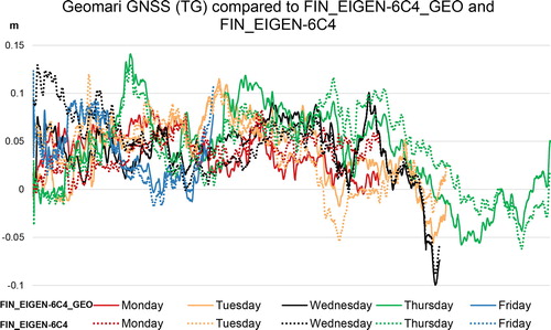
Figures 6 and 7 present the differences between geoid heights derived from the GNSS observations (TG method) and geoid models (FIN2005N00, FIN_EIGEN-6C4 and FIN_EIGEN-6C4_GEO). The results of the model with the new gravity data, FIN_EIGEN-6C4_GEO, are plotted (in solid lines) together with results of the FIN2005N00 and FIN_EIGEN-6C4 models (in dashed lines). Although the standard deviations of the daily solutions are quite similar, the figures visualize the better agreement, especially for Monday (red) and Tuesday (orange), of the GNSS tracks of Geomari with the FIN_EIGEN-6C4_GEO geoid model.

Figure 6. Differences between geoid heights derived from the GNSS observations (TG method) and geoid models after removing an offset. Solid lines present the differences with the FIN_EIGEN-6C4_GEO model. Dashed lines present the differences with the FIN2005N00 model.

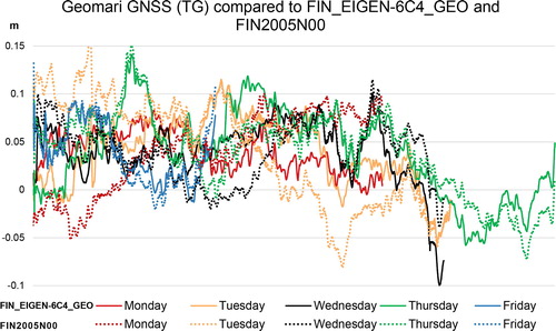
Figure 7. Differences between geoid heights derived from the GNSS observations (TG method) and geoid models after removing an offset. Solid lines present the differences with the FIN_EIGEN-6C4_GEO model. Dashed lines present the differences with the FIN_EIGEN-6C4 model.

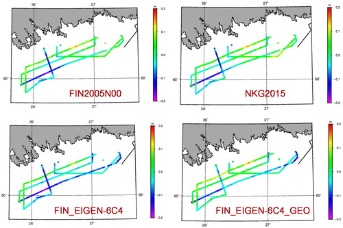
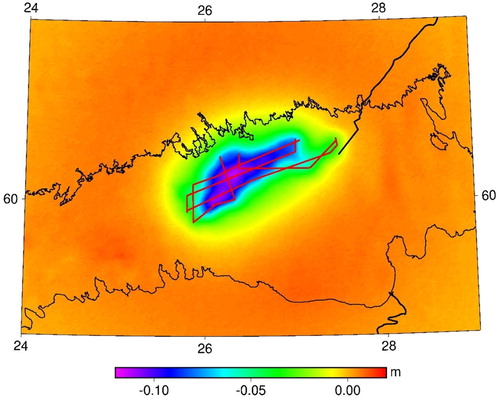
In Figure 8, the locations of the differences for the respective geoid comparisons are shown. The geoid height differences between the GNSS and geoid models are plotted along the tracks of Geomari. The plots for the FIN2005N00 (top left) and NKG2015 (top right) are quite identical and the differences to the FIN_EIGEN results (bottom part) at the eastern part of the area, where the input gravity data is different compared to the FIN_EIGEN models, are up to 10–15 cm. The differences between the FIN_EIGEN models are most prominent at the southernmost tracks: Tuesday (orange in the track plot of the Figure 1) and Friday (blue). The largest difference is seen on Friday where the geoid heights from the FIN_EIGEN-6C4_GEO differ up to 15 cm from the other geoid models.

Figure 8. Differences between the GNSS derived geoid heights and the geoid models FIN2005N00 (top left), NKG2015 (top right), FIN_EIGEN-6C4 (bottom left) and FIN_EIGEN-6C4_GEO (bottom right) along the tracks of the Geomari. An offset was removed.

Finally, to see the full effect of the new gravity data from the Geomari campaign on the geoid model in the area, we compared the old and new high-resolution FIN_EIGEN-6C4 geoid models. The models are identical, except for the gravity data from the Geomari campaign. The two models have geoid height differences up to 15 cm at the center of the campaign (Figure 9). The result coincides with the results obtained from the marine GNSS measurements (Figure 8), as GNSS derived geoid heights were able to detect the geoid discrepancies between the two geoid models. In a concluding remark, marine GNSS in combination with sea surface models has proved to be a worthy tool for validating geoid models at sea areas.

Figure 9. Differences between geoid models FIN_EIGEN-6C4 and FIN_EIGEN-6C4_GEO at the eastern part of the Gulf of Finland. Red lines are the tracks of Geomari.

Conclusions

The Geomari campaign was a marine GNSS/gravity campaign where existing geoid models were validated at sea areas by GNSS measurements in combination with sea surface models. GNSS and gravity measurements were made on the marine geology research catamaran, Geomari, in the eastern part of the Gulf of Finland in the early summer of 2018. The GNSS derived geoid heights were compared to geoid heights of the already existing geoid models FIN2005N00, NKG2015, FIN_EIGEN-6C4 and the new model FIN_EIGEN-6C4_GEO, being computed using the new gravity data collected in this research.

The daily standard deviations of the differences between the GNSS derived geoid heights and geoid models varied between 1.4 and 6.3 cm during the campaign. The best agreement to the GNSS derived geoid heights was achieved with the FIN_EIGEN models, where the daily standard deviations varied between 2.4–4.1 cm (TG) and 2.4–4.0 cm (PM). On the other hand, the daily standard deviations for the FIN2005N00 and NKG2015 models varied between 1.2–6.3 cm and 3.1–4.2, respectively. The largest daily differences between the geoid models were seen in the most eastern and southern part of the campaign. The difference can be explained by the gravity data used to calculate the respective geoid models. The FIN_EIGEN models include different data for Russia and the eastern part of the Gulf of Finland as the FIN2005N00 and the NKG2015 geoid models.

Overall, the standard deviations for the FIN_EIGEN models were quite identical. However, closer comparison along the tracks of the Geomari campaign highlighted the daily standard deviation differences up to 0.9 cm (Friday). The geoid height differences varied the most in the eastern and southern tracks, where the gravity measurements were previously sparse or non-existent. Geoid height differences of more than 10 cm were found at the southern tracks between the FIN_EIGEN models, and differences up to 15 cm when comparing the FIN_EIGEN models to the FIN2005N00 and NKG2015 along the eastern tracks.

As we compared the old and new FIN_EIGEN geoid models, geoid height differences of up to 15 cm were found. The result coincides with the results obtained from the marine GNSS measurements, as GNSS derived geoid heights were able to detect the geoid discrepancies between the two geoid models along the tracks of Geomari. Marine GNSS in combination with sea surface models has proved to be a worthy tool in validating geoid models at sea areas, as it is possible to recover geoid heights with an accuracy of a few centimetres, including the uncertainties of the geoid models.

Acknowledgements

The authors would like to send their warmest thanks to the crew of Geomari (Kimmo, Erkki and Eija), whom made the survey a reality from theory. Additionally, our sincerest thanks to the Swedish colleagues (Per-Anders and Örjan), who made the finalized gravity data from the Geomari available to us. The research was part of the FAMOS (Odin 2016–2018) project, which was co-financed by the European Union within the framework of the Connecting Europe Facility (CEF). We also thank the two anonymous reviewers, the associate editor Dr. Heiner Denker and the editor-in-chief for their valuable comments.

Additional information

Funding

European Union, Connecting Europe Facility (CEF).

References

- Ågren, J., G. Strykowski, M. Bilker-Koivula, O. Omang, S. Märdla, R. Forsberg, A. Ellmann, et al. 2016. The NKG2015 gravimetric geoid model for the Nordic-Baltic region. Presented at the Gravity, Geoid and Height Systems (GGHS), September 19–23, Thessaloniki, Greece.
- Baltic Sea Hydrographic Commission. 2020. Working Groups, BSHC Chart Datum Working Group. Accessed 5.2.2021. http://www.bshc.pro/working-groups/cdwg/.
- Barrass, C. B. 2004. Ship design and performance for masters and mates. London: Elsevier Butterworth-Heinemann.
- Bilker-Koivula, M. 2010. Development of the Finnish height conversion surface FIN2005N00. Nordic Journal of Surveying and Real Estate Research 7 (1):76–88.
- CMEMS (Copernicus Marine Environment Monitoring Service). 2016. Product user manual for Baltic Sea physical analysis and forecasting product: BALTICSEA_ANALYSIS_FORECAST_PHYS_003_006. http://cmems-resources.cls.fr/documents/PUM/CMEMS-BAL-PUM-003-006.pdf.
- FAMOS (Finalising Surveys for the Baltic Motorways of the Seas). 2020. FAMOS project, Home. http://www.famosproject.eu/.
- Geotrim. 2020. Palvelut, Trimnet VRS. https://geotrim.fi/palvelut/trimnet-vrs/.
- Häkli, P., M. Lidberg, L. Jivall, T. Nørbech, O. Tangen, M. Weber, P. Pihlak, I. Aleksejenko, and E. Paršeliūnas. 2016. The NKG2008 GPS campaign – final transformation results and a new common Nordic reference frame. Journal of Geodetic Science 6:1–33.
- Ince, E. S., C. Förste, F. Barthelmes, H. Pflug, M. Li, J. Kaminskis, K.-H. Neumayer, and G. Michalak. 2020. Gravity measurements along commercial ferry lines in the Baltic Sea and their use for geodetic purposes. Marine Geodesy 43 (6):573–602.
- Koivula, H., J. Kuokkanen, S. Marila, T. Tenhunen, P. Häkli, U. Kallio, S. Nyberg, and M. Poutanen. 2012. Finnish permanent GNSS network: From dual-frequency GPS to multi-satellite GNSS. 2012 Ubiquitous Positioning, Indoor Navigation, and Location Based Service (UPINLBS), 1–5.
- Lahtinen, S., H. Pasi, L. Jivall, C. Kempe, K. Kollo, K. Kosenko, P. Pihlak, D. Prizginiene, O. Tangen, M. Weber, et al. 2018. First results of the Nordic and Baltic GNSS analysis centre. Journal of Geodetic Science 8 (1):34–42.
- Lavrov, D., G. Even-Tzur, and J. Reinking. 2017. Expansion and improvement of the Israeli geoid model by shipborne GNSS measurements. Journal of Surveying Engineering 143 (2):04016022.
- Metsar, J., K. Kollo, and A. Ellmann. 2018. Modernization of the Estonian national GNSS reference station network. Geodesy and Cartography 44 (2):55–62.
- Nordman, M., J. Kuokkanen, M. Bilker-Koivula, H. Koivula, P. Häkli, and S. Lahtinen. 2018. Geoid validation on the Baltic Sea using ship-borne GNSS data. Marine Geodesy 41 (5):457–76.
- NovAtel. 2014. Inertial Explorer User Guide. Waypoint Products Group. https://hexagondownloads.blob.core.windows.net/public/Novatel/assets/Documents/Waypoint/Downloads/InertialExplorer860_Manual/InertialExplorer860_Manual.pdf.
- Saari, T., and M. Bilker-Koivula. 2018. Applying the GOCE-based GGMs for the quasi-geoid modelling of Finland. Journal of Applied Geodesy 12 (1):15–27.
- Varbla, S., A. Ellmann, S. Märdla, and A. Gruno. 2017. Assessment of marine geoid models by ship-borne GNSS profiles. Geodesy and Cartography 43 (2):41–9.
- Varbla, S., A. Ellmann, and N. Delpeche-Ellmann. 2020. Validation of marine geoid models by utilizing hydrodynamic model and shipborne GNSS profiles. Marine Geodesy 43 (2):134–62.