Evaluating the Suitability of Multi-Scale Terrain Attribute Calculation Approaches for Seabed Mapping Applications

Abstract

The scale dependence of benthic terrain attributes is well-accepted, and multi-scale methods are increasingly applied for benthic habitat mapping. There are, however, multiple ways to calculate terrain attributes at multiple scales, and the suitability of these approaches depends on the purpose of the analysis and data characteristics. There are currently few guidelines establishing the appropriateness of multi-scale raster calculation approaches for specific benthic habitat mapping applications. First, we identify three common purposes for calculating terrain attributes at multiple scales for benthic habitat mapping: (i) characterizing scale-specific terrain features, (ii) reducing data artefacts and errors, and (iii) reducing the mischaracterization of ground-truth data due to inaccurate sample positioning. We then define criteria that calculation approaches should fulfill to address these purposes. At two study sites, five raster terrain attributes, including measures of orientation, relative position, terrain variability, slope, and rugosity were calculated at multiple scales using four approaches to compare the suitability of the approaches for these three purposes. Results suggested that specific calculation approaches were better suited to certain tasks. A transferable parameter, termed the ‘analysis distance’, was necessary to compare attributes calculated using different approaches, and we emphasize the utility of such a parameter for facilitating the generalized comparison of terrain attributes across methods, sites, and scales.

Keywords:

• benthic habitat mapping
• geomorphometry
• multibeam echosounder
• scale
• seabed mapping
• terrain analysis

Introduction

Benthic habitat mapping approaches often seek to relate continuous-coverage environmental variables to discrete observations of seabed habitats, termed “ground-truth” observations, to predict habitat distributions over broader extents. Environmental variables may span one or multiple domains, each partly describing the environmental characteristics that determine suitable habitat for benthic organisms. These domains often include sediment properties and dynamics, physical and chemical oceanography, inter-species (i.e., community) interactions, and seabed morphology. Terrain attributes derived from bathymetric data are highly useful for describing seabed morphology, and their use has become commonplace for benthic habitat mapping. Terrain attribute calculation is a part of the field of geomorphometry, which is the science of quantitative land-surface analysis (Pike, Evans, and Hengl 2009). Given their potential utility as surrogates for ecological patterns such as biodiversity (McArthur et al. 2009, 2010; Harris 2012), surface characteristics describing the slope, orientation, relative position, and variability of the seafloor (Wilson et al. 2007; Bouchet et al. 2015) are routinely applied to predict distributions of species (e.g., Galparsoro et al. 2009; Bučas et al. 2013) and broader habitats or ‘benthoscapes’ (e.g., Brown, Sameoto, and Smith 2012; Calvert et al. 2015; Ierodiaconou et al. 2018). A high potential for surrogacy, combined with the increasing availability of high-resolution bathymetric data and user-friendly tools, has facilitated the widespread adoption of terrestrial geomorphometric techniques for marine applications over the past two decades (Lecours et al. 2016b). The calculation of raster terrain attributes from bathymetric data to describe seabed morphology can be considered part of the current quantitative predictive benthic mapping paradigm (Harris and Baker 2012; Bouchet et al. 2015).

Following several key studies on seabed morphometry (e.g., Lundblad et al. 2006; Wilson et al. 2007), and efforts to provide guidelines on marine geomorphometry (e.g., Lecours et al. 2015b; Lecours et al. 2016b; Lucieer, Lecours, and Dolan 2018), there has been progress towards establishing standards for the use of digital terrain models (DTMs) and terrain attributes for benthic habitat mapping. Fundamental concepts from terrestrial geomorphometry are now being explored in a marine context, such as spatial scale and scale-dependence of terrain attributes (e.g., Dolan and Lucieer 2014; Giusti, Innocenti, and Canese 2014; Lecours et al. 2015a; Miyamoto et al. 2017; Misiuk, Lecours, and Bell 2018), and the selection of variables and algorithms (e.g., Dolan and Lucieer 2014; Bouchet et al. 2015; Lecours et al. 2016a). The field of marine geomorphometry is further distinguished by marine-specific terrain attributes, segmentation, and classification approaches (e.g., Lundblad et al. 2006; Du Preez 2015; Di Stefano and Mayer 2018; Diesing and Thorsnes 2018; Masetti, Mayer, and Ward 2018; Walbridge et al. 2018), advances in the production of digital bathymetric models (Calder 2003; Linklater et al. 2018), and effects of DTM error and uncertainty on terrain attributes and habitat maps (e.g., Lucieer, Huang, and Siwabessy 2016; Lecours et al. 2017a; Lecours et al. 2017b). The study of these marine-specific terrain attribute characteristics has spurred the development of marine geomorphometry as a sub-discipline of geomorphometry (Lecours et al. 2018). This topic has gained traction, as highlighted by the publication of 18 articles from a special issue on marine geomorphometry in the international journal Geosciences (Lucieer, Dolan, and Lecours 2019). Its application to benthic habitat mapping has recently been highlighted by Smith Menandro and Bastos (2020), who found that ‘geomorphometry’ was one of the most used keywords for seabed mapping articles in the last decade.

Spatial scale is a fundamental concept in geomorphometry. It is well established that terrain attributes are scale-dependent – that the attributes themselves depend on the scale at which they are calculated (i.e., the scale of analysis; Woodcock and Strahler 1987; Wood 1996). The scale of terrain analysis is intrinsically linked to the source data resolution, and the highest attainable bathymetric resolution is ultimately constrained by the quality, resolution, and geometry of the raw sounding data (Hughes Clarke 2018). The finest achievable scale is not necessarily the most appropriate for every analysis though, and the calculation of seabed terrain attributes at multiple scales is increasingly common (e.g., Rengstorf et al. 2012, 2013; Giusti, Innocenti, and Canese 2014; Miyamoto et al. 2017; Misiuk, Lecours, and Bell 2018; Porskamp et al. 2018; Pearman et al. 2020; Trzcinska et al. 2020; Zelada Leon et al. 2020). Despite the increased implementation of multi-scale analyses, there is still little guidance on the appropriateness of multi-scale approaches for specific benthic habitat mapping applications. Here, we note that ‘multi-scale’ refers broadly to methods and analyses that consider multiple different spatial scales (Dolan and Lucieer 2014).

Using seabed slope as an example, Dolan and Lucieer (2014) compared five methods of multi-scale terrain attribute calculations and concluded that each method produces different results. They highlighted the challenges of determining best practices for calculating terrain attributes at variable scales, since the suitability of calculation approaches depends on the purpose of analysis and qualities of the data. Three of the multi-scale approaches (1–3 in Table 1) rely on various combinations of terrain attribute calculation using a 3 × 3 focal window and aggregating over broader spatial extents, which are simple operations in most GIS software packages. The ‘k × k-window’ method (4 in Table 1; a.k.a. ‘roving window’) differs by varying the size of the focal analysis window used to calculate the terrain attributes, which is not always straightforward to perform. There is a large potential for methodological variation since calculations differ depending on the attribute, algorithms used, and the number of cells within the k x k window to which they are applied. Options for ‘k × k-window’ calculations are not supported for many attributes in commercial software packages. Finally, several approaches have been proposed for calculating multi-scale attributes that simultaneously integrate information from multiple spatial scales in one or several layers (Method 5 in Table 1; e.g., Gallant and Dowling 2003; Schmidt and Andrew 2005; Drăguţ, Eisank, et al. 2009; Drăguţ, Schauppenlehner, et al. 2009; Wood 2009; Gorini and Mota 2011; Lindsay and Newman 2018; Shang et al. 2021). Many of these integrated methods differ fundamentally from the first four in Table 1 and are outside of the scope of this article.

Table 1. Five multi-scale approaches for calculating terrain attributes (Dolan and Lucieer 2014). Asterisks denote marine examples.

#	Method	Abbreviated name	Published examples
1	Resample DTM then calculate attribute	Resample-calculate	Rengstorf et al. (2012)*, Gottschalk et al. (2011)
2	Average DTM then calculate attribute	Average-calculate	Giusti, Innocenti, and Canese (2014)*
3	Calculate attribute then average	Calculate-average	Misiuk, Lecours, and Bell (2018)*
4	Calculate attribute using variable k × k window	k × k-window	Bargain et al. (2017)*, Porskamp et al. 2018)*, Trzcinska et al. (2020)*
5	Multiple integrated spatial scales	Integrated-multiscale	Gorini and Mota (2011), Lindsay and Newman (2018), Lecours and Espriella (2020)*, Shang et al. (2021)*

Several studies have investigated the use and effects of multi-scale calculation methods on specific terrain attributes (e.g., Dolan and Lucieer 2014; Lecours et al. 2017b; Moudrý et al. 2019), but there remains a lack of general guidelines on the appropriateness of multi-scale methods for common benthic habitat mapping applications. The goal of this paper is therefore to investigate the appropriateness of multi-scale raster calculation methods for specific scale manipulation applications, and to provide recommendations on their use. First, we identify three common purposes for manipulating the scale of terrain attributes in a benthic habitat mapping context and discuss criteria for determining the suitability of multi-scale raster calculation methods for each purpose. These purposes are then explored using several benthic terrain attributes at two study sites. The suitability of the multi-scale methods for each purpose is evaluated, and the findings are discussed to provide recommendations on their use.

Scale manipulation purpose, criteria, and methods

Purpose and criteria

There are a variety of potential reasons for manipulating the spatial scale of terrain attributes for benthic habitat mapping – here we focus on three of the most common, which are relevant to many habitat mapping studies:

1. Characterizing scale-specific terrain features. The scale of analysis may be purposefully adjusted to measure specific seabed features (e.g., dunes, reefs, pockmarks) that are poorly captured using default calculation parameters and source resolution, or to test or target scales expected to influence ecological processes of interest (e.g., Giusti, Innocenti, and Canese 2014; Gafeira, Dolan, and Monteys 2018; Porskamp et al. 2018; Zelada Leon et al. 2020). In such cases, it may be desirable to employ a method that allows the user to explicitly target terrain features at particular scales and avoid conflation with seabed features and characteristics at other scales.

2. Reducing data errors and artefacts. The scale at which terrain attributes are calculated may be adjusted (either knowingly or unknowingly) when attempting to reduce the effects of noise and acquisition artefacts in elevation or depth data (e.g., Albani et al. 2004; Gafeira, Dolan, and Monteys 2018, Buhl-Mortensen et al. 2020; Florinsky and Filippov 2021). Focal filters and resampling are used for this purpose, but they can affect the scale of analysis for measuring seabed features via terrain attributes. Naturally, these approaches aim to reduce the influence of data outliers or errors on the terrain attribute calculation, but it may also be useful, and necessary for downstream analyses, to understand the effects that filtering operations have on the scale of the attributes.

3. Matching the positional accuracy of ground-truth data. The scale of terrain attributes may be manipulated when attempting to match the positional accuracy of ground-truth data. The uncertainty of seabed sample locations can be on the order of meters or tens of meters when georeferenced from a surface platform, yet the horizontal resolution and positional accuracy of sonar data are generally much higher (Strong 2020). Where discrepancies exist between measured and actual sample locations, there is potential to mis-characterize the benthic environment by assigning incorrect terrain attribute values to ground-truth samples. The scale of terrain analysis should therefore be broader than the positional uncertainty of the ground-truth samples to avoid a spatial mismatch between terrain characterization and ground-truth information (Lecours and Devillers 2015). Terrain attributes can be generalized spatially to represent the seabed over a broader area in order to reduce the impacts of incorrect spatial matching (Sillero and Barbosa 2021), yet this may affect the scale of analysis at which the terrain is quantified. A suitable method for characterizing spatially uncertain ground-truth samples should reduce the error of terrain attribute values between measured and actual ground-truth locations with the least amount of generalization to the terrain attribute.

The suitability of the four multi-scale terrain attribute calculation methods selected (Methods 1–4, Table 1) is explored for these three purposes at two study sites of finer (km) and broader (100 s km) scales using five common benthic terrain attributes.

Datasets

D’Argent Bay

Multibeam echosounder survey of D’Argent Bay, Newfoundland and Labrador (NL), Canada, was conducted on December 4–7, 2018 and February 19–23, 2019 to provide data for benthic habitat mapping in Placentia Bay – an area designated as an Ecologically and Biologically Significant Area by Fisheries and Oceans Canada (Templeman 2007; Figure 1A). Drop camera observations at this site suggested a heterogeneous seabed primarily comprising gravel and boulder, with patches of soft sediment near the coast (Shang et al. 2021). Approximately 43 km² were mapped using a Kongsberg EM2040p (400 kHz) with differential GPS (Fugro 3610 DGNSS) aboard the research vessel D. Cartwright. Twenty-five sound velocity profiles of the water column were acquired using an AML Base X profiler for sound speed corrections. The raw multibeam data were imported to the bathymetric processing software Qimera (QPS) for post-processing. Sound velocity and tidal corrections were applied, and the data were cleaned and gridded at 5 m resolution. The 5 m raster was projected to UTM Zone 21 N to obtain metric map units for terrain attribute calculations. These data are typical of high-resolution coastal mapping surveys, and are ideal for investigating the effects of terrain attribute scale manipulation over fine spatial extents (10 s-100s of m).

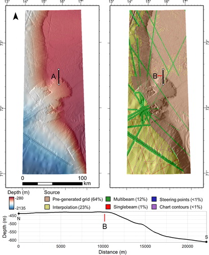
Figure 1. Locations of study sites at (A) D’Argent Bay, Newfoundland and Labrador, Canada, and (B) the Bjørnøya slide and surrounding area on the Norwegian continental margin. Source: Author, country borders were obtained from the ESRI Countries WGS84 layer.

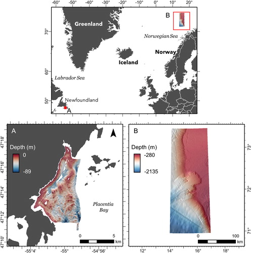
Bjørnøya slide

The General Bathymetric Chart of the Oceans (GEBCO) is the most comprehensive global bathymetric data source. Since the 2019 release, GEBCO grids have been developed through the Nippon Foundation-GEBCO Seabed 2030 Project (Mayer et al. 2018). The GEBCO dataset comprises bathymetry from multiple sources, compiled at 15 arc-second intervals. The bathymetry data, together with information on the data source, are freely available for download and are increasingly accessed as a trusted source of regional-global scale bathymetry data. Here, GEBCO_2019 bathymetry data from an example area on the Norwegian continental margin were downloaded as a broad scale case study (GEBCO Bathymetric Compilation Group 2019). The Norwegian Mapping Authority Hydrographic Service conducted multibeam surveys of the continental shelf and slope in this area during 2007–2008 as part of the national offshore mapping programme MAREANO. These data are incorporated in the GEBCO compilation, which also includes multibeam data (including transit lines) from various surveys in the area, together with background interpolated data. The otherwise smooth continental slope that dips westwards into the Norwegian Sea is incised within the study area by the 200,000- to 300,000-year-old Bjørnøya (Bear Island) slide (Laberg and Vorren 1993), which spans several tens of kilometers (Figure 1B). To the south of the slide, the upper slope includes extensive sandwave fields investigated by King et al. (2014) and Bøe et al. (2015), who also provided further details on the geological history of the area. The presence of morphological features spanning a range of scales, along with multibeam acquisition-related artefacts and distinct differences in the quality and resolution of the source bathymetric datasets, make this a relevant area to explore the consequences of multi-scale terrain analysis performed on a regional compiled dataset. The 15 arc-second GEBCO_2019 floating-point grid was projected to UTM Zone 33 N in ArcGIS Pro using bilinear interpolation to achieve square raster cells at 250 m resolution for terrain attribute calculation.

Terrain attribute calculation

The following five common terrain attributes were selected for analysis to broadly represent different classes (orientation, relative position, terrain variability, slope, rugosity, respectively; Wilson et al. 2007):

1. the eastness (sine) component of aspect,

2. relative difference to the mean value (RDMV),

3. the local standard deviation of bathymetry (SD),

4. seabed slope, and

5. vector ruggedness measure (VRM).

Each terrain attribute is readily calculated using each of the multi-scale approaches (1–4; Table 1). The effects of multi-scale calculation method are expected to be very similar for some attributes of the same class (e.g., eastness and northness components of aspect; measures of ruggedness), and redundant variables were therefore not included.

Slope and eastness were both calculated using the eight-neighbor ‘Queen’s case’ according to Horn (1981), with a custom R function to enable calculation at multiple k × k focal windows (Supplementary Material). Several configurations could be used for the slope calculation (e.g., Rook’s case according to Ritter 1987), but the Queen’s case is standard and well-accepted, generally providing a superior representation of the surface through the incorporation of elevation or depth data from the diagonals (i.e., NE, NW, SE, SW; Dolan and Lucieer 2014). RDMV and SD were calculated using the Terrain Attribute Selection for Spatial Ecology toolbox (TASSE v.1.1) for ArcGIS (Lecours 2017a), and VRM was calculated using the Benthic Terrain Modeller (BTM) toolbox (Sappington, Longshore, and Thompson 2007; Walbridge et al. 2018), both of which allow for calculation over multiple focal window sizes. Equations for all terrain attribute calculations used in this study are provided in the Appendices.

Multi-scale implementation

The ‘resample-calculate’ method for calculating terrain attributes at multiple scales (Method 1 in Table 1) was implemented using a mean aggregation within the ‘raster’ package (Hijmans 2019) in R 3.6.3 (R Core Team 2019). Equal weights were applied to all cells within a square aggregation window of size j × j for j = 1, 3, 5, …, 19 to achieve a coarser bathymetric raster for each scale of analysis. Terrain attributes were then calculated using a 3 × 3 focal window on the coarsened raster grids. The ‘average-calculate’ method (Method 2 in Table 1) was implemented by passing mean filters of dimensions j × j for j = 1, 3, 5, …, 19 over the bathymetric layers using the focal() function within the ‘raster’ package, then calculating terrain variables within a 3 × 3 focal window using the smoothed bathymetric rasters. The inverse was performed for the ‘calculate-average’ method (Method 3 in Table 1) – terrain attributes were calculated from the bathymetric rasters at their native resolution using a 3 × 3 focal window, then were smoothed using mean filters of size j × j for j = 1, 3, 5, …, 19.

The approaches used to calculate terrain attributes using these first three methods all rely on a combination of calculating the attribute within a 3 × 3 focal window and manipulating the aggregation window size j; the ‘k × k-window’ method (Method 4 in Table 1) varies the size of the focal window k used to calculate each attribute at its native resolution, and its implementation differs depending on the attribute. Eastness and slope were calculated using methods from Horn (1981), but the k × k windows were manipulated using focal weights matrices via the focal() function within the ‘raster’ package in R. Depth values were extracted from the outer eight neighbors perpendicular to, and diagonal from, the focal cell of the k × k window using the weights matrices, then were used to calculate x- and y-components of the gradient according to Horn (i.e., using half weight at the diagonals). Note that this is a simple method of calculating slope using the ‘Queen’s case’ for k × k windows larger than 3 × 3, and more intricate methods might incorporate depth information from intermediate extents of the focal window. RDMV and SD are calculable based on summary statistics of the cells within a focal window, which can therefore be expanded to any size using the TASSE toolbox. VRM is a measurement of the variability of orthogonal vectors from the raster cells within a focal window – it can also be scaled up to multiple window sizes within the BTM toolbox (Walbridge et al. 2018).

Scale manipulation parameters

It is necessary to define parameters by which the multi-scale terrain attribute methods (Table 1) can be characterized to facilitate comparison.

1. The ‘aggregation window size’, j, is the number of cells in the x and y directions over which values are aggregated for a given method. Here, aggregation refers to any generalization of terrain attribute values over a broader scale, and can therefore include any averaging or resampling of bathymetric or terrain attribute data.

2. The ‘focal window size’, k, is the number of cells in the x and y directions of the window used to calculate the terrain attribute value at the focal cell.

3. The ‘cell length’, l_c (i.e., the ‘cell size’), is the length of the cell in map units, which, for the calculation of focal terrain attributes, is normally set equal in x and y directions using an appropriate cartographic projection.

4. The ‘cell neighborhood size’, m_c, is the maximum number of cells in the x and y directions over which the value of the terrain attribute at the focal cell is affected. It can be determined by considering k, but also depends on the number of additional cells in the x or y directions that may have affected calculation at the focal cell due to other operations (e.g., aggregation; Figure 2).

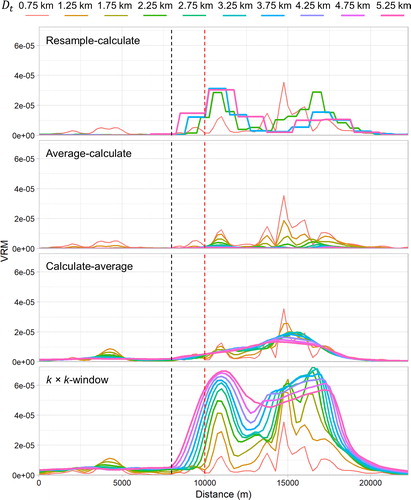
   Figure 2. Calculating raster terrain attributes at analysis distance D_t = 45 m using four different multi-scale methods: (A) ‘resample-calculate’, (B) ‘average-calculate’, (C) ‘calculate-average’, and (D) ‘k × k-window’. Parameters at the bottom of each pane describe the aggregation window size (j), focal window size (k), cell length (l_c), cell neighborhood size (m_c), and attribute calculation distance (D_i). Solid borders represent the focal cell; bold borders represent D_i. Note that for (B) and (C), the analysis distance (D_t) of calculations at the focal cell is extended to 45 m by the aggregation windows of each neighboring cell within the 3 × 3 focal window.

   

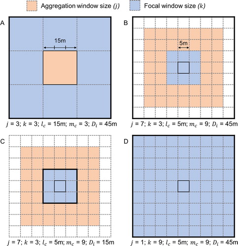
5. The ‘attribute calculation distance’, D_i, is the width of the area, in map units, over which elevation (or depth) information is incorporated at the attribute calculation step – it is unique because it depends on the order of operations in the calculation and aggregation of the attribute (e.g., whether aggregation is performed before or after calculating the terrain attribute).

6. The total ‘analysis distance’, D_t, is the maximum x and y distance in map units over which the value of the terrain attribute at the focal cell is affected. D_t is the product of the cell length and cell neighborhood size, l_c × m_c, which we note has previously been referred to as ‘scale factor’ (e.g., Lundblad et al. 2006).

These parameters are all descriptive of the different calculation methods, but the attribute calculation distance, D_i, and analysis distance, D_t, are transferable parameters that facilitate the comparison of methods. D_i describes over what distance the terrain attribute was originally calculated, or the scale of features that were quantified at the step where the attribute was calculated. If elevation or depth information is aggregated prior to calculating the attribute, or not at all, the attribute calculation distance is equal to the analysis distance (D_i = D_t). D_t is the total distance over which the calculation of a raster terrain attribute is affected. Each multi-scale method relies on manipulating the other parameters (j, k, l_c, m_c) in order to change D_t, which can, in turn, be used to organize attributes into comparable classes (e.g., Table 2). For example, resampling bathymetry then calculating the attribute adjusts D_t by manipulating the bathymetric cell length l_c over an area j × j, and this produces a greater rate of change for D_t than by maintaining a constant cell length but changing the j × j window using another method (e.g., averaging). Conversely, calculating an attribute over k × k window sizes requires a larger value of k to achieve comparable units of analysis distance as the methods that manipulate j – a source of potential confusion since both the focal and aggregation window sizes are sometimes referenced to describe the magnitude of terrain attribute rescaling, depending on the method (Moudrý et al. 2019). These parameters are not necessarily interchangeable, as demonstrated in Table 2. The total ‘analysis distance’ (D_t) is therefore a useful metric to ensure comparability between different methods and avoid ambiguity; it is used to reference the scale of terrain attributes for the remainder of this paper.

Table 2. Example of scale manipulation parameters over ten analysis distances (D_t) based on multi-scale calculation method, applied to a 5 m resolution input dataset. An example with a 250 m resolution input dataset is provided in the Appendix. Note how D_i and D_t vary relative to the other parameters and each other.

Resample bathymetry, calculate attribute (‘resample-calculate’)
Agg. window size j (cells)	1	3	5	7	9	11	13	15	17	19
Focal window size k (cells)	3	3	3	3	3	3	3	3	3	3
Cell length lc (m)	5	15	25	35	45	55	65	75	85	95
Cell neighborhood size mc (cells)	3	3	3	3	3	3	3	3	3	3
Attr. calculation distance Di (m)	15	45	75	105	135	165	195	225	255	285
Analysis distance Dt (m)	15	45	75	105	135	165	195	225	255	285
Average bathymetry, calculate attribute (‘average-calculate’)
Agg. window size j (cells)	1	3	5	7	9	11	13	15	17	19
Focal window size k (cells)	3	3	3	3	3	3	3	3	3	3
Cell length lc (m)	5	5	5	5	5	5	5	5	5	5
Cell neighborhood size mc (cells)	3	5	7	9	11	13	15	17	19	21
Attr. calculation distance Di (m)	15	25	35	45	55	65	75	85	95	105
Analysis distance Dt (m)	15	25	35	45	55	65	75	85	95	105
Calculate attribute, average attribute (‘calculate-average’)
Agg. window size j (cells)	1	3	5	7	9	11	13	15	17	19
Focal window size k (cells)	3	3	3	3	3	3	3	3	3	3
Cell length lc (m)	5	5	5	5	5	5	5	5	5	5
Cell neighborhood size mc (cells)	3	5	7	9	11	13	15	17	19	21
Attr. calculation distance Di (m)	15	15	15	15	15	15	15	15	15	15
Analysis distance Dt (m)	15	25	35	45	55	65	75	85	95	105
Calculate attribute over k × k window (‘k × k-window’)
Agg. window size j (cells)	1	1	1	1	1	1	1	1	1	1
Focal window size k (cells)	3	5	7	9	11	13	15	17	19	21
Cell length lc (m)	5	5	5	5	5	5	5	5	5	5
Cell neighborhood size mc (cells)	3	5	7	9	11	13	15	17	19	21
Attr. calculation distance Di (m)	15	25	35	45	55	65	75	85	95	105
Analysis distance Dt (m)	15	25	35	45	55	65	75	85	95	105

Comparison and statistics

Terrain attributes were compared to determine the suitability of the four multi-scale calculation methods for the three common applications and criteria addressed here. All terrain attributes were mapped at each site, and two-dimensional terrain profiles were used to visualize the change in attribute values at features of interest. The characterization of scale-specific terrain features was relevant at both sites, but the effects of calculation method on data artefacts were explored primarily at the Bjørnøya slide. Matching the positional accuracy of ground-truth sampling generally concerns high resolution datasets; this was investigated at D’Argent Bay. Select terrain attribute profiles are provided in the text, and all remaining profiles are provided in the Appendices.

Characterizing scale-specific terrain features

Identifying the most appropriate scale(s) at which to capture geomorphological features and ecological patterns has long been a goal of geomorphometry and habitat mapping, but has proven challenging in practice (Drăguţ, Eisank, et al. 2009; Lechner et al. 2012; Dove et al. 2020). A suitable method for manipulating attribute scale to match the scale of terrain features should allow for the representation of meaningful information explicitly from a given scale, and ideally, avoid conflation with terrain features at other scales.

The similarity and information content of terrain attribute values were compared to the finest analysis distance at both study sites to determine the suitability of the multi-scale methods for targeting specific scale-dependent terrain features. Pearson’s coefficient of correlation describes the linear relationship between variable pairs (i.e., similarity). It was computed between each of the nine analysis distances and the finest one for each of the five attributes to compare the redundancy of different attribute scales. Shannon’s (1948) entropy has been described as ‘a measure of the amount of information required on the average to describe the random variable’ (Cover and Thomas 2006). Entropy was calculated for each analysis distance of each attribute to compare the amounts of information retained when using the four multi-scale approaches. The entropy $H(X)$ of a discrete random variable $X$ is defined by: (1) $$H\left(X\right)=-\sum _{x}p\left(x\right)\mathrm{ log}p\left(x\right)$$(1) where $p\left(x\right)$ is the probability of observing a given data value. Given a sufficient number of observations, a continuous random variable can be quantized into bins to estimate the probability density function (Optican and Richmond 1987), which can be used to calculate the entropy (Hall and Morton 1993; Cover and Thomas 2006). Here, sample values ($n$ ≈ 0.4 and 1.4 million, respectively) of all scales of a given attribute for a given method were quantized into 1,000 bins of equal width, spanning the full range of data values to estimate the entropy. The number of bins was selected to roughly accommodate sample sizes at both study sites by balancing the bias and variance of information that is retained from the original data based on recommendations in the literature ($\sqrt{n};$ Meyer 2008). Additional bin configurations were also tested, and results were generally invariant. Quantization and entropy calculations were performed using the R package ‘infotheo’ (Meyer 2014).

Entropy values were standardized to the finest scale separately for each attribute to compare relative changes in information resulting from the different multi-scale calculation methods. A value of 1 represents the same amount of information as the finest scale; values less than or greater than 1 represent less or more entropy than the finest scale, respectively. Given the criteria for a multi-scale method that targets terrain attributes at specific, dominant scales, it would be ideal to select a method that produces attributes having low correlation with the finest scale(s) and also high information content (entropy). A low correlation with the finest scale(s) but also low entropy suggests that the attribute is not redundant, but also that it contains less information, whereby correlation may have been reduced at the cost of information content. A high correlation and high entropy suggest that the attribute is similar to the finest scale but still retains information content.

Reducing data errors and artefacts

DTM artefacts can significantly affect terrain attribute calculations (Lecours et al. 2017b) and habitat maps that are produced using affected terrain attributes (Lecours et al. 2017a). DTMs and terrain attributes are thus commonly filtered to reduce the influence of data error or artefacts on downstream map products (e.g., Novaczek, Devillers, and Edinger 2019), yet the effects of these operations on the scale of analysis are not necessarily explicit. Common DTM errors include acquisition artefacts resulting from an improper compensation of platform motion or sound velocity during acoustic surveys, artefacts caused by the imperfect integration or fusion of data from different sources (e.g., combining singlebeam echosounder data with lead line measurements and radar altimetry data), and interpolation artefacts that may introduce a gridding pattern in the data (Lecours et al. 2016b).

The effectiveness of each multi-scale calculation method was compared for reducing the effects of data errors and compilation artefacts at the Bjørnøya slide. Although it is difficult to measure the magnitude of data artefact reduction statistically, prominent compilation artefacts are often apparent from terrain attribute maps. Their locations can also be referenced using the GEBCO type identifier (TID) grid to determine where different datasets were integrated, and what methods were used for data collection – though exact data origins can be difficult to determine (e.g., data labelled as “pre-generated grid”). Terrain profiles at a distinct slide feature and a data compilation boundary were used to explore the effects of the different calculation methods on apparent errors and known compilation artefacts. Values of terrain attributes at the profiles were plotted for the ten analysis distances to observe the effects of the multi-scale methods on the influence of data errors for terrain attribute calculations.

Matching the positional accuracy of ground-truth data

The disparity between positional accuracy of sonar data and ground-truth samples can be problematic when using terrain attributes to characterize the benthic environment, and may introduce error that negatively impacts downstream habitat maps (Gábor et al. 2020; Strong 2020). While the positional accuracy of sonar soundings is constrained primarily by the positioning, synchronization, and motion compensation systems of the acquisition platform, positional uncertainty of ground-truth data can be influenced by additional sources such as equipment drift from the vessel. Methods and technologies exist to increase the positional accuracy of benthic ground-truth data (e.g., line out calculation, ultra-short baseline), yet it may not always be possible to match the accuracy of sonar-derived terrain data given the acquisition platform, sampling equipment, and water depth (Lecours and Devillers 2015). Ground-truth data from global databases like the Ocean Biogeographic Information System (OBIS) can also have very low positional accuracy (Moudrý and Devillers 2020) compared to bathymetric data. As a result, error in ground-truth data positioning can cause mischaracterization of the benthic environment, wherein ground-truth observations are assigned incorrect terrain attribute values based on the measured sample position, which differs from the actual position, which is not known. The effect may become more severe when characterizing the terrain at finer scales (Gábor et al. 2020).

One method for mitigating such mischaracterization is to coarsen, or generalize, the terrain attributes to reflect the spatial uncertainty associated with the ground-truth samples. Such operations will generally also affect the scale of terrain attributes though, and this should be carefully considered in the context of the analysis. For example, in cases where it is desirable to quantify the terrain at fine scales, it is important to seek a method for reducing spatial precision of terrain variables that maintains a fine scale of analysis. Such cases may motivate an efficient reduction in spatial precision, which impacts the scale of analysis minimally.

Spatially uncertain benthic sampling was simulated at the D’Argent Bay site to investigate the efficiency with which the spatial precision of terrain attributes can be reduced to avoid ground-truth mischaracterization. First, 1,000 sample points simulating the ‘actual’ locations of ground-truth samples were randomly generated within the area of multibeam coverage at D’Argent Bay. Each sample point was assigned a spatial buffer of 20 m radius, within which a second point was randomly generated, representing the ‘measured’ sample location, which differs from the ‘actual’ by a horizontal error of up to 20 m. Values of all five terrain attributes were extracted at both points across the ten analysis distances (D_t), as calculated using each of the four multi-scale methods. The difference between terrain attribute values for each sample pair (‘actual’ – ‘measured’) was calculated to represent the potential error for each sample, given maximum hypothetical positional errors of 0–20 m. Errors between the four multi-scale calculation methods were compared at each analysis distance.

Case study results

Characterizing scale-specific terrain features

Features at a variety of spatial scales can be resolved from the D’Argent Bay dataset. At the finest scale, topographic complexity can be captured from only a few neighboring cells at 5 m resolution (Figure 3). A terrain profile illustrates how these are superimposed on broader topographic features that span tens to hundreds of meters (Figure 3A). At the broadest scales, features can be observed that span hundreds or thousands of meters – almost the length of the entire study site.

Figure 3. Hillshaded 5 m resolution bathymetry at D’Argent Bay. A terrain profile from West to East (A) shows topographic features at several scales. Finer-scale features are superimposed on broader ones (B).

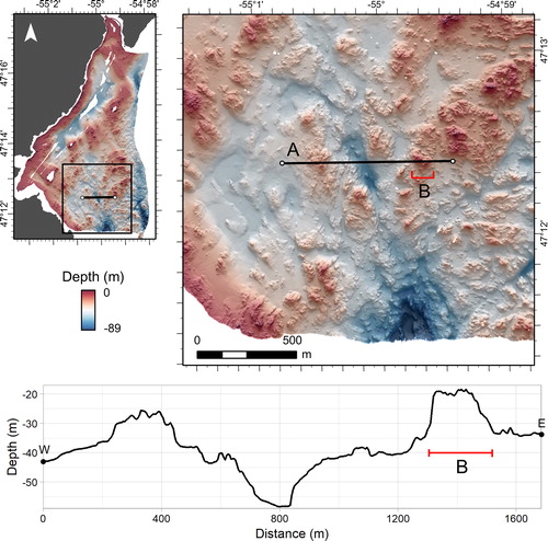
The four terrain attribute calculation methods tested produced different results for this dataset. The topographic position of the mounds, trenches, and the features they contain can be characterized using RDMV. Using the ‘average-calculate’ and ‘calculate-average’ methods, fine-scale features are smoothed out at analysis distances greater than 15 m (Figure 4). Of these two methods, the former retains some information at moderate analysis distances (e.g., D_t = 45 to 75 m), suggesting general topographic highs and lows, while the latter has smoothed out nearly all detail. RDMV calculated using the variable ‘k × k-window’ method enables identification of the two 50–75 m high points on the mound identified in Figure 3B, which, importantly, are separated by a topographically negative feature. Similarly, the ‘resample-calculate’ method enables the identification of features at distinct scales, albeit at a decreased horizontal resolution (i.e., greater cell length). From this terrain profile, it appears that both ‘resample-calculate’ and ‘k × k-window’ methods are effective at identifying topographic position at distinct scales using RDMV. However, we note that none of the layers in Figure 4 are at broad enough scales to identify the entire mound as a topographic high. The analysis distance, D_t, enables comparison of the maximum horizontal extent of the RDMV layer (D_t = 105 m) with that of the mound (width ≈ 200 m). A broader analysis distance would therefore be required to describe this feature.

Figure 4. Relative difference to the mean value (RDMV) at the transect in Figure 3A across ten analysis distances (D_t) using four different multi-scale calculation methods at D’Argent Bay. Values at the finest scale (red) describe correspondingly small topographic features; values at moderate (green) and broad (purple) scales differ substantially between methods. Dashed lines indicate the extent of the feature indicated in Figure 3B.

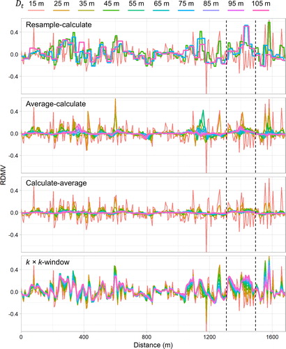
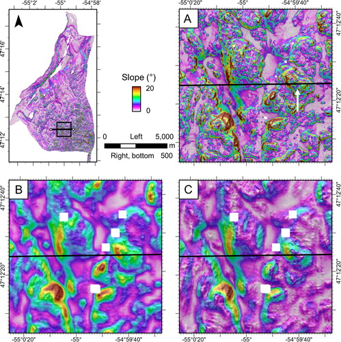
Though subtler than with RDMV, the slopes of features along the profile in Figure 3 also exhibit different values when calculated at multiple scales using the four methods (Figure 5). One important difference is that the ‘calculate-average’ method fails to characterize flat sections of topographic highs and lows – instead averaging the slope value across the entire feature. This is apparent from the slope map, where flat areas are poorly defined at the 65 m analysis distance compared to the ‘k × k-window’ method (Figure 6).

Figure 5. Slope at the transect in Figure 3 calculated across ten analysis distances (D_t) using four different multi-scale calculation methods at D’Argent Bay. Slope details and flat areas are averaged out using the ‘calculate-average’ method. Dashed lines indicate the extent of the feature indicated in Figure 3B.

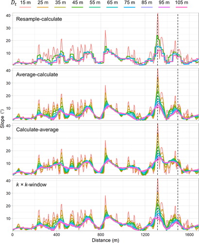
Figure 6. Hillshaded slope at D’Argent Bay. The magnified area shows features along the terrain profile. At analysis distance D_t = 15 m (A), an arrow indicates the feature discussed in the text and annotated in Figure 3. The scale of the slope layers is increased to D_t = 65 m using (B) ‘calculate-average’ and (C) ‘k × k-window’ methods. The color ramp is clipped to a maximum of 20° to facilitate comparison between maps.

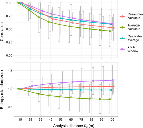
All methods produced attributes of decreasing correlation with the finest scale, yet entropy values of the ‘resample-calculate’ and ‘k × k-window’ attributes exceeded those of the finest scale, on average (Figure 7). Entropy values were generally invariant to increases in analysis distance with the ‘calculate-average’ method. Although ‘average-calculate’ attributes had the lowest correlation scores of any method, entropy values decreased markedly with increasing analysis distance, suggesting a loss of information. This conforms with observations of terrain attributes along the profile (e.g., Figure 4), which show that the variability of attributes was often greatly reduced at broad scales. Similar findings were observed at the Bjørnøya slide (Appendices), yet we note that correlation and entropy statistics at both sites were variable between attributes. All correlation and entropy statistics for the individual attributes and methods are provided in the Supplementary Material.

Figure 7. Average correlation and entropy statistics of terrain attributes compared to the finest scale using each multi-scale calculation method at D’Argent Bay. Error bars show the standard deviations of all variables at each analysis distance.

Reducing data errors and artefacts

The Bjørnøya slide dataset contains features at a variety of scales, but also artefacts resulting from multisource data compilation. These include linear artefacts remaining from multibeam data processing and surface generation, boundary discrepancies between datasets of different sources, and combinations of data of variable source resolutions – for example, multibeam data overlaying broader interpolation (Figure 8). Focal filters may be used to mitigate the influence of such artefacts, yet the incorporation of depth information from surrounding raster cells affects the scale of subsequent terrain attribute calculations. The ‘average-calculate’ method, for example, can be conceptualized as a focal filter followed by terrain attribute calculation, and it is informative to examine this operation in the context of the other multi-scale calculation methods.

Figure 8. Hillshaded 250 m resolution GEBCO bathymetry (left) and data source identified via type identifier (TID) grid (right) at the Bjørnøya slide. A terrain profile from North to South (A; bottom) crosses what appears to be a dataset compilation boundary (at B) near the crown of the slide. Note that the pre-generated grid sections contain multiple data sources and are not necessarily of uniform quality/resolution. The pre-generated grid data south of B comprise full-coverage multibeam bathymetry from which more consistent terrain attributes are expected.

At the finest analysis distance (D_t = 750 m), compilation artefacts are apparent in the RDMV layer over much of the study area, or are indistinguishable from bathymetric features (Figure 9B). Although the ‘resample-calculate’ method effectively highlights extensive topographic features at broader scales, compilation artefacts are obvious at many locations (Figure 9C). Perhaps more nefarious than obvious artefacts, though, is the confusion between artefacts and physical features, which can severely impact downstream mapping applications (e.g., species/habitat distribution models, benthoscape maps). The ‘k × k-window’ method also performed well at characterizing broader topographic features, yet compilation artefacts have been propagated to broader scales (Figure 9F). The other two methods – ‘average-calculate’ and ‘calculate-average’ – contrast with the former two. RDMV maps demonstrate a loss of detail at broader scales, affecting both the terrain representation and compilation artefacts (Figure 9D, E). This is corroborated by terrain profiles and results from section “Characterizing scale-specific terrain features”, which suggested a loss of information resulting from these two approaches (Appendices).

Figure 9. Effects of terrain attribute calculation methods on multisource data compilation (A) artefacts at the Bjørnøya slide. Relative difference to the mean value (RDMV) and eastness at analysis distance D_t = 750 m (B, G) are increased to D_t = 3,750 using ‘resample-calculate’ (C, H), ‘average-calculate’ (D, I), ‘calculate-average’ (E, J), and ‘k × k-window’ (F, K) methods. The data compilation boundary identified in Figure 8 is indicated by the dashed red line in (A).

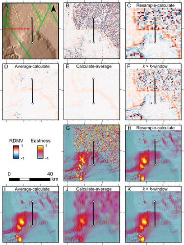
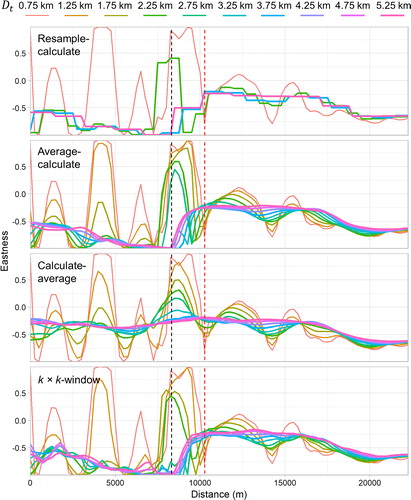
The eastness at the finest analysis distance (D_t = 750 m) also appears to be substantially impacted by the various data compilation artefacts at the slide location (Figure 9G). At coarser scales, these effects manifest differently depending on the multi-scale calculation method, but at all scales, data compilation artefacts are easily confused with actual features. At analysis distance D_t = 3,750 m, ‘resample-calculate’, ‘average-calculate’, and ‘k × k-window’ maps all look similar, unlike those of RDMV. The maps produced using these methods also suggest that, in addition to smoothing out data artefacts, the eastness of broader terrain features is now being quantified. The ‘calculate-average’ layer is the most distinct (Figure 9J); fine-scale variability and acquisition line artefacts are still apparent north of the slide and broader features are not quantified. The finer-scale features and artefacts have been averaged with surrounding data to suggest a less easterly orientation than indicated by the other methods north of the slide.

For eastness, the attribute calculation distance (D_i), which describes over what distance the terrain attribute is initially quantified, appears to profoundly affect how the terrain is represented at broader scales. ‘Calculate-average’ is the only method here in which D_i is not equal to the total analysis distance, D_t, and it is apparent that broad-scale terrain features are less distinct compared to the other methods (Figure 9; Appendices). The terrain profile at the top of the slide that crosses the boundary of two datasets – potentially of different source resolutions – shows that averaging the values of the more variable northern section obscures the broader-scale changes in aspect that are apparent from the other layers (Figure 10). In essence, by calculating the attribute before aggregating it, the ‘calculate-average’ method takes a local consensus of what the value of the attribute is at the finest scale. The profile suggests that the ‘resample-calculate’ and ‘average-calculate’ methods quantify broader-scale terrain features while smoothing the variability in the northern section of the dataset, while the ‘k × k-window’ method quantifies broader-scale terrain features but does a poor job at smoothing the data.

Figure 10. Eastness from North to South (left to right) at the profile in Figures 8 and 9 calculated across ten analysis distances (D_t) using four different multi-scale calculation methods at the Bjørnøya slide. Vertical dashed lines show approximate locations of the slide crown (black) and dataset compilation boundary (red).

These observations generally hold for the other attributes that aim to measure some aspect of terrain variability (i.e., SD, VRM). ‘Resample-calculate’ and ‘k × k-window’ methods retained a higher level of information describing both terrain detail and compilation artefacts. The ‘average-calculate’ method consistently produced a decrease in detail (both of terrain and artefacts) at broader scales. The terrain detail and artefacts of attributes resulting from the ‘calculate-average’ method were inconsistent depending on the attribute, likely as a result of the variable effect that the artefacts have on the different attribute calculations (since the calculation is performed prior to the smoothing operation – i.e., averaging or aggregating). All terrain attribute maps and profiles at both study sites are provided in the Appendices.

Matching the positional accuracy of ground-truth data

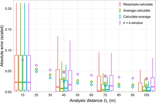
The ‘calculate-average’ method was consistently efficient at reducing errors caused by sample location uncertainty. Figure 11 demonstrates that even with a modest increase in analysis distance (e.g., from 15 to 45 m), the mean error between ‘actual’ and ‘measured’ terrain attribute values can be reduced to levels comparable to those achieved at the coarsest scales using ‘k × k-window’ and ‘resample-calculate’ methods. The ‘k × k-window’ method performed comparatively poorly at reducing positionally induced errors, with both higher and more variable errors than the other methods. Results from the ‘resample-calculate’ method are more nuanced; although box plots show that this method effectively reduced much of the error caused by spatially inaccurate sampling as measured by the median, the means of the absolute error suggest the influence of extreme outliers. This discrepancy is suspected to be caused by an increasing proportion of sample pairs (‘actual’ and ‘measured’) occurring in the same raster cell with increasing cell size, which reduces the error between them to zero. However, if sample pairs occur across cell borders, there is a large error between the ‘measured’ and ‘actual’ terrain attribute values. The magnitude of this discrepancy appears to increase with scale (Figure 11). In contrast, the more gradational methods (i.e., ‘average-calculate’, ‘calculate-average’) are accommodating to locational error reduction across a range of scales, with a more consistent relationship between the mean of the absolute error and the remainder of the error distribution.

Figure 11. Scaled (0-1) absolute error between all terrain attribute values at ‘actual’ and ‘measured’ sample sites for multiple analysis distances at D’Argent Bay. Box plots show the error distributions at analysis distances that can be achieved using all multi-scale calculation methods (i.e., including ‘resample-calculate’), with means at all scales displayed as circles.

Discussion and recommendations

The analysis of seabed morphology is an important component to characterizing benthic habitat, and there is a strong need to better resolve the effects of terrain attribute rescaling operations that are commonly applied in that context. Previous research has demonstrated the disparity between results from different multi-scale calculation methods (Dolan and Lucieer 2014), and the importance of spatial scale in benthic habitat mapping is generally recognized (Lecours et al. 2015a). There has also been increased interest in methods for testing and implementing terrain attributes at multiple scales for benthic habitat mapping (e.g., Rengstorf et al. 2012; Giusti, Innocenti, and Canese 2014; Miyamoto et al. 2017; Misiuk, Lecours, and Bell 2018; Porskamp et al. 2018). Given the increased uptake of these methods, and lack of existing guidelines, the goal of this paper was to investigate the appropriateness of multi-scale calculation approaches for three common habitat mapping applications.

The fitness-for-use or fitness-for-purpose of these approaches ultimately depends on a combination of the terrain attribute, data quality, and project goals (Devillers et al. 2007; Dolan and Lucieer 2014; Pôças et al. 2014), yet we note qualities, based on these results, that may help to distinguish the relative suitabilities of these approaches (Table 3). Generally, the ‘resample-calculate’ and ‘k × k-window’ methods performed similarly for the three applications. The ‘average-calculate’ and ‘calculate-average’ methods also performed similarly to each other.

Table 3. Comparison of relative suitability of multi-scale calculation methods for the three purposes identified in this study.

Purpose	Criteria	Multi-scale method performance				Comments
		Resample- calculate	Average- calculate	Calculate- average	k × k- window
Characterize specific features or processes.	Maximize new and unique information at the target scale.	Good	Poor	Poor	Good	‘k × k’ and ‘resample-calculate’ methods were effective. Selection depends on the desired resolution.
Reduce data compilation artefacts.	Minimize influence of artefacts on the terrain attribute.	Mixed	Mixed	Mixed	Poor	‘Average-calculate’ reduced the magnitude of artefacts, but also reduced terrain information.
Match positional accuracy of ground-truth.	Minimize error between terrain attribute values at ‘measured’ and ‘actual’ sample locations.	Poor	Good	Good	Poor	‘Calculate-average’ provided the greatest reduction in sample locational error.

The ‘resample-calculate’ and ‘k × k-window’ methods were both effective at characterizing specific scale-dependent features at both sites in this study. Correlation and entropy statistics demonstrated that these methods effectively provided new information that was not represented at the native analysis distance, and this was corroborated by observations of the attribute maps and terrain profiles. An interesting characteristic linking ‘resample-calculate’ and ‘k × k-window’ methods is that once the cell length has been adjusted for ‘resample-calculate’, the size of the focal window k, in map units, is equal to that of the ‘k × k-window’ method at a given analysis distance (e.g., Figure 2). It is likely that using an attribute calculation distance (D_i) equal to the total analysis distance (D_t) is important in this context, which allows for the integration of depth information at the full analysis extent. We recommend that either of these approaches be selected for the purpose of characterizing scale-specific features – selection between the two may be determined by the desired cell length.

Differences in the effectiveness at reducing data noise and artefacts between these methods were less straightforward to interpret. The ‘k × k-window’ method appeared to perform poorly at reducing data artefacts in nearly all cases. Results between the other three methods were mixed – largely depending on the variable in question. The ‘average-calculate’ method appeared to reduce the magnitude of errors consistently, but this almost always corresponded to a loss of morphological detail. It is unclear whether the artefact reduction, relative to the amount of detail loss, was superior to the other methods. It is therefore difficult to recommend any of these approaches generally for artefact reduction, though they may be effective for specific variables and datasets. We suggest that generally, other purpose-built methods such as median, low-pass, or Fourier filtering may be preferable for consistent and general-purpose artefact reduction (e.g., Wilken et al. 2012).

The methods most useful for describing features at specific scales were less effective at matching positionally-uncertain ground-truth samples simulated in this study, and vice-versa. Implicit in the goal of describing scale-specific features is that new information must be captured from different spatial extents. This goal is essentially counter to that of matching the positional uncertainty of ground-truth, which is to generalize terrain attribute values at a given measured location so that any seabed sample proximal to that location will not be mischaracterized. The ‘calculate-average’ method performed best for matching positionally uncertain ground-truth, relying exclusively on localized information for the terrain attribute calculation, which is subsequently generalized. Results suggested that, all else being equal, this method was the most efficient at minimizing the error between the measured terrain attribute values and the actual, given a spatial discrepancy of up to 20 m.

The link between spatial precision and the terrain attribute scale should be considered even when manipulating the scale of analysis is not the primary goal of the operation. It is possible, for example, to reduce spatial precision by simply characterizing broader-scale features – thereby increasing the likelihood that actual ground-truth locations occur on the same terrain features as measured from the erroneous sample geolocation. However, it may be preferable to quantify features at the native scale then generalize (i.e., ‘smooth’) values over a broader area if a finer scale of analysis is desired. The difference between these approaches can be understood from the attribute calculation distance (D_i) and analysis distance (D_t) parameters. If precision is to be reduced by characterizing broader-scale features, then an increase in analysis distance can be attained using any method in which D_t and D_i are equal (e.g., ‘resample-calculate’, ‘average-calculate’, ‘k × k-window’), meaning that the terrain attribute calculation is performed using elevation information from a broader area. Results here suggest that the ‘average-calculate’ method may be a suitable approach, whereas variable ‘k × k-windows’ may be a poor choice (Figure 11). If maintaining a fine attribute scale is desirable though, the calculation distance, D_i, can be fixed, followed by manipulation of D_t (e.g., the ‘calculate-average’ method), wherein only local elevation information is used at the calculation step.

This concept highlights the importance of the order of operations in multi-step terrain attribute calculations, emphasizing the difference, for example, between ‘calculate-average’ and ‘average-calculate’ methods. The order in which the aggregation and calculation are performed dictates the distance over which attributes are initially calculated (D_i). The subsequent generalization of the attribute values to a broader analysis distance does not affect the distance at which they were initially derived, which has implications for the application of the calculated attributes. For example, slope calculated from 5 m cells using a 3 × 3 focal window, which is then averaged over a 7 × 7 aggregation window, produces an analysis distance D_t = 45 m, but does not represent the slope of the full 45 m area (e.g., Figure 2). The slope of this area can be measured using any method wherein depth information from the 45 m area is incorporated in the slope calculation – in other words, where the calculation distance (D_i) is equal to the analysis distance (D_t) of the attribute (‘average-calculate’, ‘resample-calculate, ‘k × k-window’ methods). This aligns with the apparent usefulness of the ‘resample-calculate and ‘k × k-window’ methods for characterizing scale-specific terrain features found in this study.

In addition to facilitating comparison of different multi-scale terrain calculation methods, transferable parameters such as analysis distance (D_t) are useful for determining the appropriate attribute scale for describing specific terrain features. For example, structurally complex environments may support elevated levels of biodiversity by providing attachment surfaces for epifauna and shelter for other organisms (Ross et al. 2007; Buhl-Mortensen et al. 2010; McArthur et al. 2010). If the scale of structural features such as rocky outcrop, boulder, or coral mounds is known – for example, through direct observation or high-resolution surveying (Diesing and Thorsnes 2018) – the analysis distance can be set appropriately to match the feature scale. Although seabed mapping studies that employ multi-scale terrain characterization commonly state the focal (k × k) or aggregation (j × j) window sizes used for the calculations, this does a comparatively poor job of describing at what spatial scale features are being quantified. The analysis distance (D_t) describes the distance over which terrain attribute values are affected in map units, and depends on an interplay between cell length (l_c), aggregation window size (j), and focal window size (k).

Only a few configurations of the scale parameters used to calculate analysis distance are presented here (Table 2), yet the complexity of tracking these can be increased depending on the treatment of the bathymetric data or the selection of alternative raster calculation approaches. For example, depth data might initially be aggregated (using one of many focal filters or resampling techniques) and then used to calculate attributes over variable k × k-windows, complicating the tracking of D_i and D_t. Additionally, all terrain attribute calculations here are assumed to use square aggregation and focal windows (j × j; k × k), while these can actually assume different shapes (e.g., circle, donut), which may even be asymmetric (e.g., oval, rectangle), potentially affecting the determination of the parameters or causing them to vary with direction. Using asymmetric cases, scale parameters may be anisotropic, and can be calculated in multiple directions if necessary. Common cases are considered here to focus on the implications of multi-scale calculation methods. While these additional possibilities may frustrate the tracking of multi-scale terrain attribute calculation parameters in some instances, it may be highly advisable for applications such as matching ground-truth uncertainty while maintaining a certain analysis distance. We also note other alternatives to multi-scale terrain attribute calculation methods that differ fundamentally from those presented here, such as quadratic surface estimation (Evans 1972; Wood 1996). The analysis distance is still attainable in such cases – though it may vary with location (Shang et al. 2021).

A diverse set of terrain attributes were calculated to investigate the three scale manipulation purposes identified in this paper, yet it is important to note that while these findings (Table 3) may be transferable to similar applications, they also may vary given different goals and dataset characteristics. For other applications, or even other terrain attributes, it is important to reassess the purpose of scale manipulation in that context. For similar applications though, findings here may be highly relevant – even for terrestrial analogs such as selecting appropriate predictor scale and balancing the scale of analysis with DTM error (e.g., Florinsky and Kuryakova 2000; Albani et al. 2004; Bradter et al. 2013), or handling sources of sample location uncertainty (Gábor et al. 2019). Furthermore, the manipulation of scale is not limited to terrain characterization. Methods for characterizing benthic substrates from acoustic backscatter features have also implemented multi-scale approaches, (Blondel and Gómez Sichi 2009; Robert, Jones, and Huvenne 2014; Janowski et al. 2018; Zelada Leon et al. 2020), and Malik (2019) has demonstrated the importance of slope scale on acoustic backscatter estimation. Regardless of the application, the appropriateness of multi-scale methods must be carefully assessed given the context and data characteristics.

‘Integrated-multiscale’ terrain attribute calculation methods (Method 5 in Table 1) have not been discussed here in detail, yet they may offer several advantages over fixed-scale approaches for benthic habitat mapping. By incorporating terrain information from multiple spatial scales simultaneously, redundancies may be avoided that may otherwise hinder the use of terrain attributes at multiple separate scales for statistical modelling and classification (e.g., multicollinearity, multi-dimensionality, variable interpretability). ‘Integrated-multiscale’ methods may also help to maximize the amount of relevant terrain information for predictive models, simultaneously avoiding subjective scale selection and potentially simplifying the variable selection process. An outstanding difficulty on the generalized application of such approaches for seabed mapping, though, is an expansive methodological variation between specific attributes and software implementations. It is currently unclear whether any given approach can be applied universally to different terrain attributes, and whether any such generalizable approach is preferable to others for specific benthic habitat mapping applications (e.g., benthoscape mapping, habitat distribution modelling, unsupervised classification) or geomorphological characterisation. These topics warrant future research.

Conclusions

Implicit in any comparison of terrain attribute scale is that the parameters used to perform the attribute calculations are transferable across different calculation methods. We stress the importance of using a generalized parameter for such comparisons, and propose the analysis distance (D_t) as a straightforward, interpretable metric that relates directly to the scale of analysis in map units. We encourage the use of D_t as a terrain attribute descriptor to increase the transferability and interpretability of mapping results that utilize multi-scale terrain analysis methods.

Having organized terrain attributes calculated using different multi-scale methods according to analysis distance, results suggest important differences between methods that help to define their suitability for three common habitat mapping applications. The ‘k × k-window’ and ‘resample-calculate’ methods were generally successful at targeting distinct seabed terrain features at variable scales. In contrast, the ‘average-calculate’ method was most consistent at reducing data artefacts, but we note that this comes at the cost of reducing the information content of the terrain attribute. Simulations also suggested that the latter method was effective at reducing ground-truth characterization error due to inaccurate positioning, as was the ‘calculate-average’ method, which produced the greatest reduction in error. The calculation of “analysis distance” for these attributes allows for their direct comparison and facilitates understanding of the effects of different methods on the scale of terrain feature characterization.

Acknowledgements

Thank you to the Fisheries and Marine Institute’s School of Ocean Technology and Centre for Applied Ocean Technology for access to the boat and technical personnel and to Kirk Regular and Eugene Antle for D’Argent Bay data collection. Thank you to Alexandre Schimel for comments and suggestions on the manuscript.

Disclosure statement

The authors declare no competing interests.

Data availability statement

The GEBCO_2019 bathymetry data supporting the findings in this study are available for free from the GEBCO data portal: https://www.gebco.net/data_and_products/gridded_bathymetry_data/gebco_2019/gebco_2019_info.html. Access to the D’Argent Bay multibeam data will be considered upon request by the authors.

Correction Statement

This article has been republished with minor changes. These changes do not impact the academic content of the article.

Additional information

Funding

This work was partly supported by Fisheries and Oceans Canada’s Coastal Environmental Baseline Program and by a Canada Research Chair program through a chair in Ocean Mapping to KR. BM was partially supported by the Fisheries and Marine Institute’s School of Ocean Technology, and by an International Postdoctoral Fellowship awarded through the Ocean Frontier Institute/Canada First Research Excellence Fund. Funds allocated to VL by the University of Florida Senior Vice President for Agriculture and Natural Resources were used to support collaboration with BM at the University of Florida School of Forest, Fisheries, and Geomatics Sciences.

Appendices

Appendix 1: terrain attribute equations

Eastness

The aspect of the focal cell is defined by (A1) $$a=\mathrm{atan}2\left(\frac{\mathrm{d}z}{\mathrm{d}y},-\frac{\mathrm{d}z}{\mathrm{d}x}\right)\frac{180}{\pi }$$(A1) where $\frac{\mathrm{d}z}{\mathrm{d}y}$ and $\frac{\mathrm{d}z}{\mathrm{d}x}$ are rates of depth change in the y and x directions, respectively. These were determined here using eight weighted neighbors at the outer extents of the focal window (Horn 1981). Aspect is then converted to compass direction using the rules (A2) $$a_c=\{\begin{array}{c}90-a,\mathrm{ }a\le 90\\ 450-a,\mathrm{ }a>90\mathrm{ }\end{array}$$(A2) and eastness is given by the sine of the aspect in radians: (A3) $$\mathit{eastness}=\text{sin}\left(\frac{a_c\pi }{180}\right).$$(A3)

RDMV

The relative difference to the mean value (RDMV) is a unitless measure of topographic position of the focal cell within the focal window. It is defined by (A4) $$\mathit{RDMV}=\frac{-\left(\overline{z}-z_c\right)}{z_{\mathit{max}}-z_{\mathit{min}}}$$(A4) where $\overline{z}$ is the mean depth of cells in the focal window, $z_c$ is the depth of the focal cell, and $z_{\mathit{max}}$ and $z_{\mathit{min}}$ are the maximum and minimum depth values within the focal window, respectively. Positive RDMV values, therefore, indicate locally elevated cells and negative values indicate local depressions.

Standard deviation

The bathymetric standard deviation is calculated by (A5) $$SD=\sqrt{\frac{\sum {\left(z_i-\overline{z}\right)}^2}{k^2}}$$(A5) where $z_i$ are depth values of each cell within the focal window, $\overline{z}$ is the mean depth of cells in the focal window, and $k$ is the focal window size.

Slope

Slope in degrees is defined by (A6) $$\mathit{slope}=\frac{180}{\pi }\left(\arctan \sqrt{{\left(\frac{\mathrm{d}z}{\mathrm{d}x}\right)}^2+{\left(\frac{\mathrm{d}z}{\mathrm{d}y}\right)}^2}\right)$$(A6) where $\frac{\mathrm{d}z}{\mathrm{d}x}$ and $\frac{\mathrm{d}z}{\mathrm{d}y}$ are rates of depth change in the x and y directions, respectively. These were determined using eight weighted neighbors at the outer extents of the focal window (Horn 1981).

VRM

The vector ruggedness measure (VRM) calculation is described in detail by Sappington, Longshore, and Thompson (2007). The entire land (or seabed) surface is first decomposed into unit vectors orthogonal to each grid cell, using the slope and aspect: (A7) $${xy}_i=\text{sin}\left({\alpha }_i\right),$$(A7) (A8) $$x_i={xy}_i\text{sin}\left({\beta }_i\right),$$(A8) (A9) $$y_i={xy}_i\text{cos}\left({\beta }_i\right),$$(A9) and (A10) $$z_i=\text{cos}\left({\alpha }_i\right)$$(A10) where ${\alpha }_i$ and $\beta$ are the slope and aspect at each grid cell. The VRM for a given focal window is then defined by (A11) $$\mathit{VRM}=1-\frac{\sqrt{{\left(\sum x_i\right)}^2+{\left(\sum y_i\right)}^2+{\left(\sum z_i\right)}^2}}{k^2}$$(A11) where $k$ is the size of the focal window.

Appendix 2: Bjørnøya slide scale parameters

Table A1. Example of scale manipulation parameters over ten analysis distances (D_t) based on multi-scale calculation method, applied to a 250 m resolution input dataset.

Resample bathymetry, calculate attribute (‘resample-calculate’)
Agg. window size j (cells)	1	3	5	7	9	11	13	15	17	19
Focal window size k (cells)	3	3	3	3	3	3	3	3	3	3
Cell length lc (m)	250	750	1250	1750	2250	2750	3250	3750	4250	4750
Cell neighborhood size mc (cells)	3	3	3	3	3	3	3	3	3	3
Attr. calculation distance Di (m)	750	2250	3750	5250	6750	8250	9750	11250	12750	14250
Analysis distance Dt (m)	750	2250	3750	5250	6750	8250	9750	11250	12750	14250
Average bathymetry, calculate attribute (‘average-calculate’)
Agg. window size j (cells)	1	3	5	7	9	11	13	15	17	19
Focal window size k (cells)	3	3	3	3	3	3	3	3	3	3
Cell length lc (m)	250	250	250	250	250	250	250	250	250	250
Cell neighborhood size mc (cells)	3	5	7	9	11	13	15	17	19	21
Attr. calculation distance Di (m)	750	1250	1750	2250	2750	3250	3750	4250	4750	5250
Analysis distance Dt (m)	750	1250	1750	2250	2750	3250	3750	4250	4750	5250
Calculate attribute, average attribute (‘calculate-average’)
Agg. window size j (cells)	1	3	5	7	9	11	13	15	17	19
Focal window size k (cells)	3	3	3	3	3	3	3	3	3	3
Cell length lc (m)	250	250	250	250	250	250	250	250	250	250
Cell neighborhood size mc (cells)	3	5	7	9	11	13	15	17	19	21
Attr. calculation distance Di (m)	750	750	750	750	750	750	750	750	750	750
Analysis distance Dt (m)	750	1250	1750	2250	2750	3250	3750	4250	4750	5250
Calculate attribute over k × k window (‘k × k-window’)
Agg. window size j (cells)	1	1	1	1	1	1	1	1	1	1
Focal window size k (cells)	3	5	7	9	11	13	15	17	19	21
Cell length lc (m)	250	250	250	250	250	250	250	250	250	250
Cell neighborhood size mc (cells)	3	5	7	9	11	13	15	17	19	21
Attr. calculation distance Di (m)	750	1250	1750	2250	2750	3250	3750	4250	4750	5250
Analysis distance Dt (m)	750	1250	1750	2250	2750	3250	3750	4250	4750	5250

Appendix 3: Bjørnøya slide correlation and entropy statistics

Figure A1. Average correlation and entropy statistics of terrain attributes compared to the finest scale using each multi-scale calculation method at the Bjørnøya slide. Standard deviations are shown by the error bars.

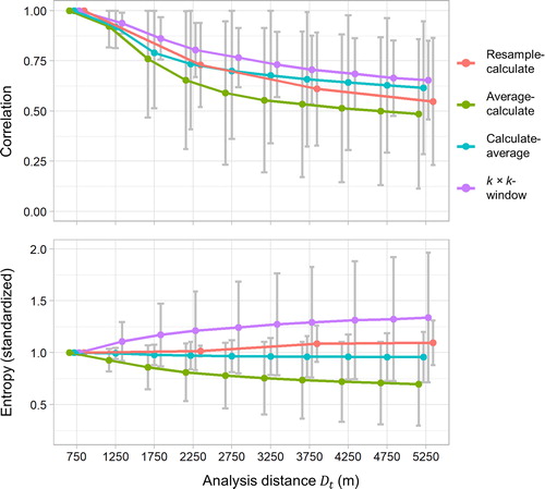
Appendix 4: D’Argent Bay terrain attribute maps

Figure A2. Eastness at D’Argent Bay at analysis distance D_t = 15 m (A) is increased to D_t = 65 m using (B) ‘resample-calculate’, (C) ‘average-calculate’, (D) ‘calculate-average’, and (E) ‘k × k-window’ methods.

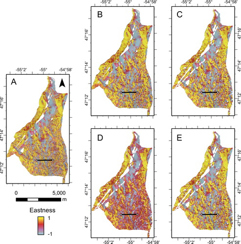
Figure A3. Relative difference to the mean value (RDMV) at D’Argent Bay at analysis distance D_t = 15 m (A) is increased to D_t = 65 m using (B) ‘resample-calculate’, (C) ‘average-calculate’, (D) ‘calculate-average’, and (E) ‘k × k-window’ methods.

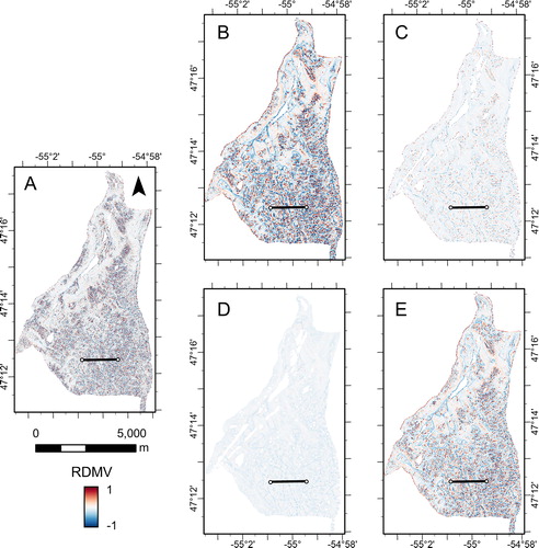
Figure A4. Bathymetric standard deviation at D’Argent Bay at analysis distance D_t = 15 m (A) is increased to D_t = 65 m using (B) ‘resample-calculate’, (C) ‘average-calculate’, (D) ‘calculate-average’, and (E) ‘k × k-window’ methods.

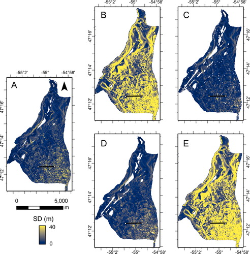
Figure A5. Slope at D’Argent Bay at analysis distance D_t = 15 m (A) is increased to D_t = 65 m using (B) ‘resample-calculate’, (C) ‘average-calculate’, (D) ‘calculate-average’, and (E) ‘k × k-window’ methods.

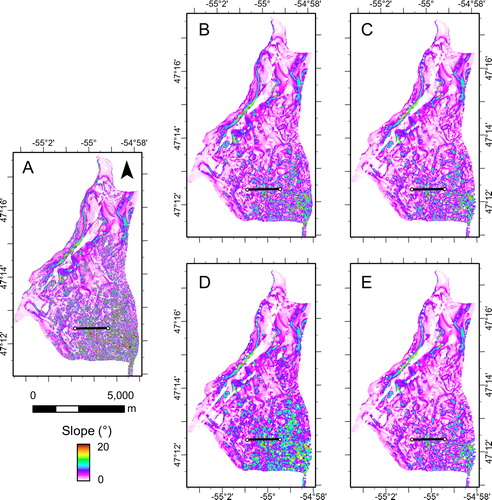
Figure A6. Vector ruggedness measure (VRM) at D’Argent Bay at analysis distance D_t = 15 m (A) is increased to D_t = 65 m using (B) ‘resample-calculate’, (C) ‘average-calculate’, (D) ‘calculate-average’, and (E) ‘k × k-window’ methods.

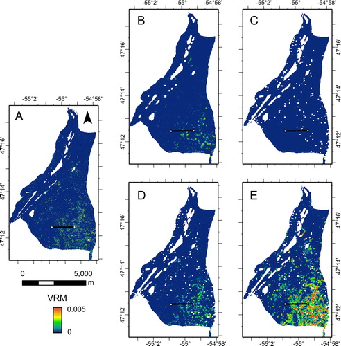
Appendix 5: D’Argent Bay terrain attribute profiles

Figure A7. Eastness at the transect in Figure 3 calculated across 10 analysis distances (D_t) using four different multi-scale methods at D’Argent Bay.

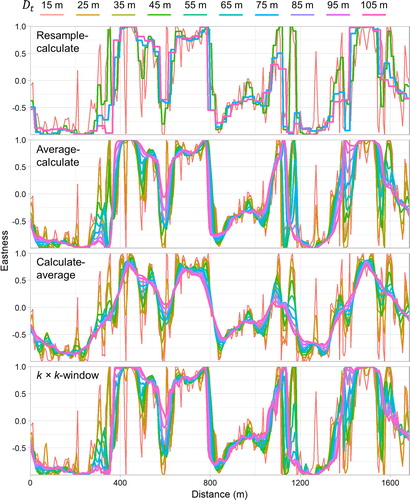
Figure A8. Bathymetric standard deviation at the transect in Figure 3 calculated across 10 analysis distances (D_t) using four different multi-scale methods at D’Argent Bay.

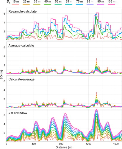
Figure A9. Vector ruggedness measure (VRM) at the transect in Figure 3 calculated across 10 analysis distances (D_t) using four different multi-scale methods at D’Argent Bay.

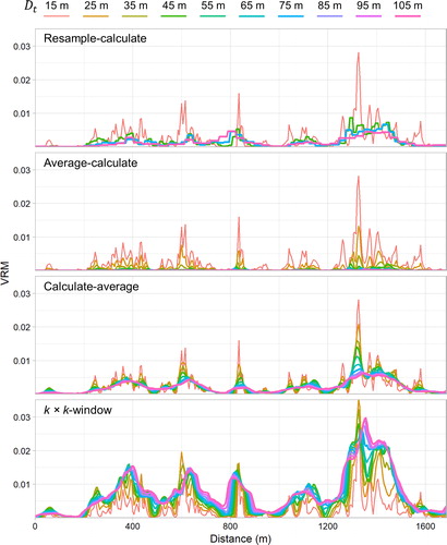
Appenidx 6: Bjørnøya slide terrain attribute maps

Figure A10. Eastness at the Bjørnøya slide at analysis distance D_t = 750 m (A) is increased to D_t = 3,750 m using (B) ‘resample-calculate’, (C) ‘average-calculate’, (D) ‘calculate-average’, and (E) ‘k × k-window’ methods.

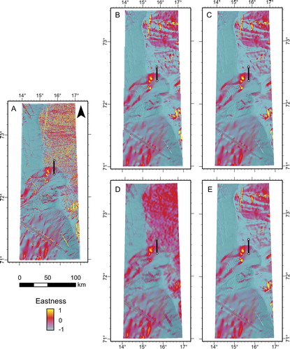
Figure A11. Relative difference to the mean value (RDMV) at the Bjørnøya slide at analysis distance D_t = 750 m (A) is increased to D_t = 3,750 m using (B) ‘resample-calculate’, (C) ‘average-calculate’, (D) ‘calculate-average’, and (E) ‘k × k-window’ methods.

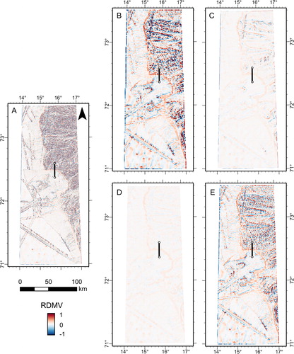
Figure A12. Bathymetric standard deviation at the Bjørnøya slide at analysis distance D_t = 750 m (A) is increased to D_t = 3,750 m using (B) ‘resample-calculate’, (C) ‘average-calculate’, (D) ‘calculate-average’, and (E) ‘k × k-window’ methods.

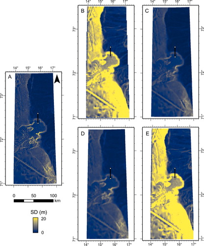
Figure A13. Slope at the Bjørnøya slide at analysis distance D_t = 750 m (A) is increased to D_t = 3,750 m using (B) ‘resample-calculate’, (C) ‘average-calculate’, (D) ‘calculate-average’, and (E) ‘k × k-window’ methods.

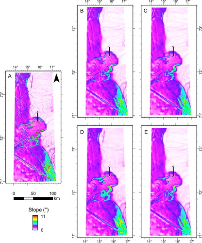
Figure A14. Vector ruggedness measure (VRM) at the Bjørnøya slide at analysis distance D_t = 750 m (A) is increased to D_t = 3,750 m using (B) ‘resample-calculate’, (C) ‘average-calculate’, (D) ‘calculate-average’, and (E) ‘k × k-window’ methods.

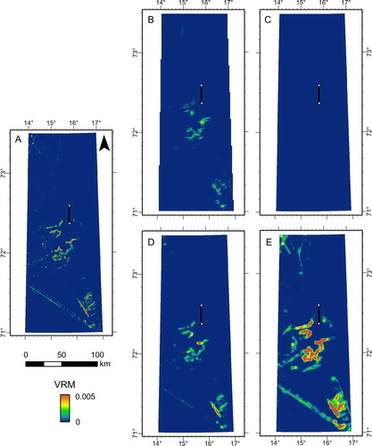
Appendix 7: Bjørnøya slide terrain attribute profiles

Figure A15. Relative difference to the mean value (RDMV) from North to South (left to right) at the profile in Figure 8 calculated across 10 analysis distances (D_t) using four different multi-scale methods at the Bjørnøya slide. Vertical dashed lines show approximate locations of the slide crown (black) and dataset compilation boundary (red).

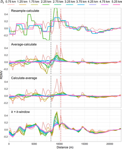
Figure A16. Bathymetric standard deviation from North to South (left to right) at the profile in Figure 8 calculated across 10 analysis distances (D_t) using four different multi-scale methods at the Bjørnøya slide. Vertical dashed lines show approximate locations of the slide crown (black) and dataset compilation boundary (red).

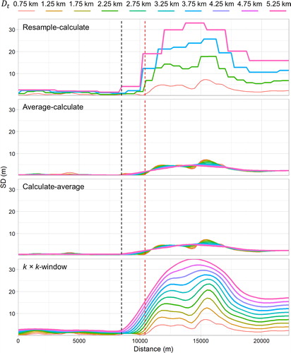
Figure A17. Slope from North to South (left to right) at the profile in Figure 8 calculated across 10 analysis distances (D_t) using four different multi-scale methods at the Bjørnøya slide. Vertical dashed lines show approximate locations of the slide crown (black) and dataset compilation boundary (red).

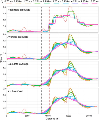
Figure A18. Vector ruggedness measure (VRM) from North to South (left to right) at the profile in Figure 8 calculated across 10 analysis distances (D_t) using four different multi-scale methods at the Bjørnøya slide. Vertical dashed lines show approximate locations of the slide crown (black) and dataset compilation boundary (red).

References

- Albani, M., B. Klinkenberg, D. W. Andison, and J. P. Kimmins. 2004. The choice of window size in approximating topographic surfaces from digital elevation models. International Journal of Geographical Information Science 18 (6):577–93.
- Bargain, A., F. Marchese, A. Savini, M. Taviani, and M.-C. Fabri. 2017. Santa Maria di Leuca Province (Mediterranean Sea): Identification of suitable mounds for cold-water coral settlement using geomorphometric proxies and Maxent methods. Frontiers in Marine Science 4:338.
- Blondel, P., and O. Gómez Sichi. 2009. Textural analyses of multibeam sonar imagery from Stanton Banks. Northern Ireland Continental Shelf. Applied Acoustics 70 (10):1288–97.
- Bøe, R., J. Skarðhamar, L. Rise, M. F. J. Dolan, V. K. Bellec, M. Winsborrow, Ø. Skagseth, J. Knies, E. L. King, O. Walderhaug, et al. 2015. Sandwaves and sand transport on the Barents Sea continental slope offshore northern Norway. Marine and Petroleum Geology 60:34–53.
- Bouchet, P. J., J. J. Meeuwig, C. P. Salgado Kent, T. B. Letessier, and C. K. Jenner. 2015. Topographic determinants of mobile vertebrate predator hotspots: Current knowledge and future directions. Biological Reviews 90 (3):699–728.
- Bradter, U., W. E. Kunin, J. D. Altringham, T. J. Thom, and T. G. Benton. 2013. Identifying appropriate spatial scales of predictors in species distribution models with the random forest algorithm. Methods in Ecology and Evolution 4 (2):167–74.
- Brown, C. J., J. A. Sameoto, and S. J. Smith. 2012. Multiple methods, maps, and management applications: Purpose made seafloor maps in support of ocean management. Journal of Sea Research 72:1–13.
- Bučas, M., U. Bergström, A.-L. Downie, G. Sundblad, M. Gullström, M. von Numers, A. Šiaulys, and M. Lindegarth. 2013. Empirical modelling of benthic species distribution, abundance, and diversity in the Baltic Sea: Evaluating the scope for predictive mapping using different modelling approaches. ICES Journal of Marine Science 70 (6):1233–43.
- Buhl-Mortensen, P., M. F. J. Dolan, R. E. Ross, G. Gonzalez-Mirelis, L. Buhl-Mortensen, L. R. Bjarnadóttir, and J. Albretsen. 2020. Classification and mapping of benthic biotopes in Arctic and sub-Arctic Norwegian waters. Frontiers in Marine Science 7:271.
- Buhl-Mortensen, L., A. Vanreusel, A. J. Gooday, L. A. Levin, I. G. Priede, P. Buhl-Mortensen, H. Gheerardyn, N. J. King, and M. Raes. 2010. Biological structures as a source of habitat heterogeneity and biodiversity on the deep ocean margins: Biological structures and biodiversity. Marine Ecology 31 (1):21–50.
- Calder, B. 2003. Automatic statistical processing of multibeam echosounder data. International Hydrographic Review 4 (1).
- Calvert, J., J. A. Strong, M. Service, C. McGonigle, and R. Quinn. 2015. An evaluation of supervised and unsupervised classification techniques for marine benthic habitat mapping using multibeam echosounder data. ICES Journal of Marine Science 72 (5):1498–513.
- Cover, T. M., and J. A. Thomas. 2006. Elements of Information Theory. 2nd ed. Hoboken, N.J: Wiley-Interscience.
- Devillers, R., Y. Bédard, R. Jeansoulin, and B. Moulin. 2007. Towards spatial data quality information analysis tools for experts assessing the fitness for use of spatial data. International Journal of Geographical Information Science 21 (3):261–82.
- Di Stefano, M., and L. Mayer. 2018. An automatic procedure for the quantitative characterization of submarine bedforms. Geosciences 8 (1):28.
- Diesing, M., and T. Thorsnes. 2018. Mapping of cold-water coral carbonate mounds based on geomorphometric features: An object-based approach. Geosciences 8 (2):34.
- Dolan, M. F. J., and V. L. Lucieer. 2014. Variation and uncertainty in bathymetric slope calculations using geographic information systems. Marine Geodesy 37 (2):187–219.
- Dolan, M. F. J., T. Thorsnes, J. Leth, Z. Al-Hamdani, J. Guinan, and V. Van Lancker. 2012. Terrain Characterization from Bathymetry Data at Various Resolutions in European Waters - Experiences and Recommendations. NGU Report. Trondheim, Norway: Geological Survey of Norway.
- Dove, D., R. Nanson, L. R. Bjarnadóttir, J. Guinan, J. Gafeira, A. Post, M. F. J. Dolan, H. Stewart, R. Arosio, and G. Scott. 2020. A Two-Part Seabed Geomorphology Classification Scheme (v.2); Part 1: Morphology Features Glossary (version 2). Zenodo. 10.5281/zenodo.4075248
- Drăguţ, L., C. Eisank, T. Strasser, and T. Blaschke. 2009. A comparison of methods to incorporate scale in geomorphometry. In Proceedings of Geomorphometry 2009. Zurich, Switzerland.
- Drăguţ, L., T. Schauppenlehner, A. Muhar, J. Strobl, and T. Blaschke. 2009. Optimization of scale and parametrization for terrain segmentation: An application to soil-landscape modeling. Computers & Geosciences 35 (9):1875–83.
- Du Preez, C. 2015. A new arc–chord ratio (ACR) rugosity index for quantifying three-dimensional landscape structural complexity. Landscape Ecology 30 (1):181–92.
- Espriella, M. C., V. Lecours, P. C. Frederick, E. V. Camp, and B. Wilkinson. 2020. Quantifying intertidal habitat relative coverage in a Florida estuary using UAS imagery and GEOBIA. Remote Sensing 12 (4):677.
- Evans, I. S. 1972. General geomorphometry, derivatives of altitude, and descriptive statistics. In Spatial Analysis in Geomorphology, ed. R.J. Chorley, 17–90. Methuen, London: Routledge.
- Florinsky, I. V., and S. V. Filippov. 2021. Three-dimensional geomorphometric modeling of the Arctic Ocean submarine topography: A low-resolution desktop application. IEEE Journal of Oceanic Engineering 46 (1):1–14.
- Florinsky, I. V., and G. A. Kuryakova. 2000. Determination of grid size for digital terrain modelling in landscape investigations—exemplified by soil moisture distribution at a micro-scale. International Journal of Geographical Information Science 14 (8):815–32.
- Gábor, L., V. Moudrý, V. Barták, and V. Lecours. 2019. How do species and data characteristics affect species distribution models and when to use environmental filtering? International Journal of Geographical Information Science 34 (8):1–18.
- Gábor, L., V. Moudrý, V. Lecours, M. Malavasi, V. Barták, M. Fogl, P. Šímová, D. Rocchini, and T. Václavík. 2020. The effect of positional error on fine scale species distribution models increases for specialist species. Ecography 43 (2):256–69.
- Gafeira, J., M. F. J. Dolan, and X. Monteys. 2018. Geomorphometric characterization of pockmarks by using a GIS-based semi-automated toolbox. Geosciences 8 (5):154.
- Gallant, J. C., and T. I. Dowling. 2003. A multiresolution index of valley bottom flatness for mapping depositional areas. Water Resources Research 39 (12).
- Galparsoro, I., Á. Borja, J. Bald, P. Liria, and G. Chust. 2009. Predicting suitable habitat for the European lobster (Homarus gammarus), on the Basque continental shelf (Bay of Biscay), using Ecological-Niche Factor Analysis. Ecological Modelling 220 (4):556–67.
- GEBCO Bathymetric Compilation Group. 2019. The GEBCO_2019 Grid - a continuous terrain model of the global oceans and land. British Oceanographic Data Centre. National Oceanography Centre, NERC, UK.
- Giusti, M., C. Innocenti, and S. Canese. 2014. Predicting suitable habitat for the gold coral Savalia savaglia (Bertoloni, 1819) (Cnidaria, Zoantharia) in the South Tyrrhenian Sea. Continental Shelf Research 81:19–28.
- Gorini, M. A. V., and G. L. A. Mota. 2011. Which is the best scale? Finding fundamental features and scales in DEMs. In Proceedings of Geomorphometry 2011, 67–70. Redlands, CA.
- Gottschalk, T. K., B. Aue, S. Hotes, and K. Ekschmitt. 2011. Influence of grain size on species–habitat models. Ecological Modelling 222 (18):3403–12.
- Hall, P., and S. C. Morton. 1993. On the estimation of entropy. Annals of the Institute of Statistical Mathematics 45 (1):69–88.
- Harris, P. T. 2012. Surrogacy. In Seafloor geomorphology as benthic habitat, ed. P.T. Harris and E.K. Baker, 93–108. Amsterdam: Elsevier.
- Harris, P. T., and E. K. Baker. 2012. GeoHab atlas of seafloor geomorphic features and benthic habitats: Synthesis and lessons learned. In Seafloor geomorphology as benthic habitat, ed. P. T. Harris and E. K. Baker, 871–90. Amsterdam: Elsevier.
- Hijmans, R. J. 2019. Raster: Geographic Data Analysis and Modeling. R (version 2.8-19). https://CRAN.R-project.org/package=raster.
- Horn, B. K. P. 1981. Hill shading and the reflectance map. Proceedings of the IEEE 69 (1):14–47.
- Hughes Clarke, J. 2018. The impact of acoustic imaging geometry on the fidelity of seabed bathymetric models. Geosciences 8 (4):109.
- Ierodiaconou, D., A. C. G. Schimel, D. Kennedy, J. Monk, G. Gaylard, M. Young, M. Diesing, and A. Rattray. 2018. Combining pixel and object based image analysis of ultra-high resolution multibeam bathymetry and backscatter for habitat mapping in shallow marine waters. Marine Geophysical Research 39 (1–2):2: 271–288. no
- Janowski, L., K. Trzcinska, J. Tegowski, A. Kruss, M. Rucinska-Zjadacz, and P. Pocwiardowski. 2018. Nearshore benthic habitat mapping based on multi-frequency, multibeam echosounder data using a combined object-based approach: A case study from the Rowy site in the southern Baltic Sea. Remote Sensing 10 (12):1983.
- King, E. L., R. Bøe, V. K. Bellec, L. Rise, J. Skarðhamar, B. Ferré, and M. F. J. Dolan. 2014. Contour current driven continental slope-situated sandwaves with effects from secondary current processes on the Barents Sea margin offshore Norway. Marine Geology 353:108–27.
- Laberg, J. S., and T. O. Vorren. 1993. A Late Pleistocene submarine slide on the Bear Island Trough Mouth Fan. Geo-Marine Letters 13 (4):227–34.
- Lechner, A. M., W. T. Langford, S. D. Jones, S. A. Bekessy, and A. Gordon. 2012. Investigating species–environment relationships at multiple scales: Differentiating between intrinsic scale and the modifiable areal unit problem. Ecological Complexity 11:91–102.
- Lecours, V. 2017b. On the use of maps and models in conservation and resource management (Warning: Results may vary). Frontiers in Marine Science 4:288.
- Lecours, V., C. J. Brown, R. Devillers, V. L. Lucieer, and E. N. Edinger. 2016a. Comparing selections of environmental variables for ecological studies: A focus on terrain attributes. PLoS ONE 11 (12):e0167128.
- Lecours, V., and R. Devillers. 2015. Assessing the spatial data quality paradox in the deep-sea. In Proceedings of Spatial Knowledge and Information - Canada (SKI-Canada), 1–8. Banff, AB.
- Lecours, V., R. Devillers, E. N. Edinger, C. J. Brown, and V. L. Lucieer. 2017a. Influence of artefacts in marine digital terrain models on habitat maps and species distribution models: A multiscale assessment. Remote Sensing in Ecology and Conservation 3 (4):232–46.
- Lecours, V., R. Devillers, V. L. Lucieer, and C. J. Brown. 2017b. Artefacts in marine digital terrain models: A multiscale analysis of their impact on the derivation of terrain attributes. IEEE Transactions on Geoscience and Remote Sensing 55 (9):5391–406.
- Lecours, V., R. Devillers, D. C. Schneider, V. L. Lucieer, C. J. Brown, and E. N. Edinger. 2015a. Spatial scale and geographic context in benthic habitat mapping: Review and future directions. Marine Ecology Progress Series 535:259–84.
- Lecours, V., M. F. J. Dolan, A. Micallef, and V. L. Lucieer. 2016b. A review of marine geomorphometry, the quantitative study of the seafloor. Hydrology and Earth System Sciences 20 (8):3207–44.
- Lecours, V., V. L. Lucieer, M. F. J. Dolan, and A. Micallef. 2015b. An ocean of possibilities: Applications and challenges of marine geomorphometry. In Geomorphometry for geosciences, ed. J. Jasiewicz, Z. Zwoliński, H. Mitasova, and T. Hengl. Poznań. Poznań: Adam Mickiewicz University in Poznań - Institute of Geoecology and Geoinformation.
- Lecours, V., V. L. Lucieer, M. F. J. Dolan, and A. Micallef. 2018. Recent and future trends in marine geomorphometry. In Proceedings of Geomorphometry 2018, 1–4. Boulder, CO.
- Lecours, V. 2017a. TASSE (Terrain Attribute Selection for Spatial Ecology) Toolbox v. 1.1. http://rgdoi.net/10.13140/RG.2.2.15014.52800.
- Lindsay, J. B., and D. R. Newman. 2018. Hyper-scale analysis of surface roughness. Preprint. PeerJ Preprints. https://peerj.com/preprints/27110v1.
- Linklater, M., S. M. Hamylton, B. P. Brooke, S. L. Nichol, A. R. Jordan, and C. D. Woodroffe. 2018. Development of a seamless, high-resolution bathymetric model to compare reef morphology around the subtropical island shelves of Lord Howe Island and Balls Pyramid, southwest Pacific Ocean. Geosciences 8 (1):11.
- Lucieer, V., M. Dolan, and V. Lecours. eds. 2019. Marine Geomorphometry. Basel: MDPI. https://doi.org/10.1007/s10980-016-0374-x.
- Lucieer, V., Z. Huang, and J. Siwabessy. 2016. Analyzing uncertainty in multibeam bathymetric data and the impact on derived seafloor attributes. Marine Geodesy 39 (1):32–52.
- Lucieer, V., V. Lecours, and M. F. J. Dolan. 2018. Charting the course for future developments in marine geomorphometry: An introduction to the special issue. Geosciences 8 (12):477.
- Lundblad, E. R., D. J. Wright, J. Miller, E. M. Larkin, R. Rinehart, D. F. Naar, B. T. Donahue, S. M. Anderson, and T. Battista. 2006. A benthic terrain classification scheme for American Samoa. Marine Geodesy 29 (2):89–111.
- Malik, M. 2019. Sources and impacts of bottom slope uncertainty on estimation of seafloor backscatter from swath sonars. Geosciences 9 (4):183.
- Masetti, G., L. A. Mayer, and L. G. Ward. 2018. A bathymetry- and reflectivity-based approach for seafloor segmentation. Geosciences 8 (1):14.
- Mayer, L., M. Jakobsson, G. Allen, B. Dorschel, R. Falconer, V. Ferrini, G. Lamarche, H. Snaith, and P. Weatherall. 2018. The Nippon Foundation—GEBCO Seabed 2030 Project: The quest to see the world’s oceans completely mapped by 2030. Geosciences 8 (2):63.
- McArthur, M. A., B. Brooke, R. Przeslawski, D. A. Ryan, V. L. Lucieer, S. Nichol, A. W. McCallum, C. Mellin, I. D. Cresswell, and L. C. Radke. 2009. A Review of Abiotic Surrogates for Marine Benthic Biodiversity. Canberra: Geoscience Australia.
- McArthur, M. A., B. P. Brooke, R. Przeslawski, D. A. Ryan, V. L. Lucieer, S. Nichol, A. W. McCallum, C. Mellin, I. D. Cresswell, and L. C. Radke. 2010. On the use of abiotic surrogates to describe marine benthic biodiversity. Estuarine, Coastal and Shelf Science 88 (1):21–32.
- Meyer, P. E. 2008. Information-theoretic variable selection and network inference from microarray data. PhD Thesis., Brussels, Belgium: Universite Libre de Bruxelles.
- Meyer, P. E. 2014. Infotheo: Information-Theoretic Measures. R (version 1.2.0). https://CRAN.R-project.org/package=infotheo.
- Misiuk, B., V. Lecours, and T. Bell. 2018. A multiscale approach to mapping seabed sediments. PLoS ONE 13 (2):e0193647.
- Miyamoto, M., M. Kiyota, H. Murase, T. Nakamura, and T. Hayashibara. 2017. Effects of bathymetric grid-cell sizes on habitat suitability analysis of cold-water gorgonian corals on seamounts. Marine Geodesy 40 (4):205–23.
- Moudrý, V., and R. Devillers. 2020. Quality and usability challenges of global marine biodiversity databases: An example for marine mammal data. Ecological Informatics 56:101051.
- Moudrý, V., V. Lecours, M. Malavasi, B. Misiuk, L. Gábor, K. Gdulová, P. Šímová, and J. Wild. 2019. Potential pitfalls in rescaling digital terrain model-derived attributes for ecological studies. Ecological Informatics 54:100987.
- Novaczek, E., R. Devillers, and E. Edinger. 2019. Generating higher resolution regional seafloor maps from crowd-sourced bathymetry. PLoS ONE 14 (6):e0216792.
- Optican, L. M., and B. J. Richmond. 1987. Temporal encoding of two-dimensional patterns by single units in primate inferior temporal cortex. III. Information theoretic analysis. Journal of Neurophysiology 57 (1):162–78.
- Pearman, T. R. R., K. Robert, A. Callaway, R. Hall, C. Lo Iacono, and V. A. I. Huvenne. 2020. Improving the predictive capability of benthic species distribution models by incorporating oceanographic data – Towards holistic ecological modelling of a submarine canyon. Progress in Oceanography 184:102338.
- Pike, R. J., I. S. Evans, and T. Hengl. 2009. Geomorphometry: A brief guide. In Developments in soil science, ed. M. Busse, C. P. Giardina, D. M. Morris, and D. S. Page-Dumroese, 33:3–30. Amsterdasm: Elsevier. https://linkinghub.elsevier.com/retrieve/pii/S0166248108000019.
- Pôças, I., J. Gonçalves, B. Marcos, J. Alonso, P. Castro, and J. P. Honrado. 2014. Evaluating the fitness for use of spatial data sets to promote quality in ecological assessment and monitoring. International Journal of Geographical Information Science 28 (11):2356–71.
- Porskamp, P., A. Rattray, M. Young, and D. Ierodiaconou. 2018. Multiscale and hierarchical classification for benthic habitat mapping. Geosciences 8 (4):119.
- R Core Team. 2019. R: A Language and Environment for Statistical Computing (version 3.5.3). Vienna, Austria: R Foundation for Statistical Computing.
- Rengstorf, A. M., A. Grehan, C. Yesson, and C. Brown. 2012. Towards high-resolution habitat suitability modeling of vulnerable marine ecosystems in the deep-sea: Resolving terrain attribute dependencies. Marine Geodesy 35 (4):343–61.
- Rengstorf, A. M., C. Yesson, C. Brown, and A. J. Grehan. 2013. High-resolution habitat suitability modelling can improve conservation of vulnerable marine ecosystems in the deep sea. Journal of Biogeography 40 (9):1702–14.
- Ritter, P. 1987. A vector-based slope and aspect generation algorithm. Photogrammetric Engineering & Remote Sensing 53 (8):1109–11.
- Robert, K., D. O. B. Jones, and V. A. I. Huvenne. 2014. Megafaunal distribution and biodiversity in a heterogeneous landscape: The iceberg-scoured Rockall Bank, NE Atlantic. Marine Ecology Progress Series 501:67–88.
- Ross, P. M., S. F. Thrush, J. C. Montgomery, J. W. Walker, and D. M. Parsons. 2007. Habitat complexity and predation risk determine juvenile snapper (Pagrus auratus) and goatfish (Upeneichthys lineatus) behaviour and distribution. Marine and Freshwater Research 58 (12):1144–51.
- Sappington, J. M., K. M. Longshore, and D. B. Thompson. 2007. Quantifying landscape ruggedness for animal habitat analysis: A case study using bighorn sheep in the Mojave Desert. Journal of Wildlife Management 71 (5):1419–26.
- Schmidt, J., and R. Andrew. 2005. Multi-scale landform characterization. Area 37 (3):341–50.
- Shang, X., K. Robert, B. Misiuk, J. Mackin-McLaughlin, and J. Zhao. 2021. Self-adaptive analysis scale determination for terrain features in seafloor substrate classification. Estuarine, Coastal and Shelf Science 254:107359.
- Shannon, C. E. 1948. A mathematical theory of communication. Bell System Technical Journal 27 (3):379–423.
- Sillero, N., and A. M. Barbosa. 2021. Common mistakes in ecological niche models. International Journal of Geographical Information Science 35 (2):213–4.
- Smith Menandro, P., and A. C. Bastos. 2020. Seabed mapping: A brief history from meaningful words. Geosciences 10 (7):273.
- Strong, J. A. 2020. An error analysis of marine habitat mapping methods and prioritised work packages required to reduce errors and improve consistency. Estuarine, Coastal and Shelf Science 240:106684.
- Templeman, N. D. 2007. Placentia Bay-Grand banks large ocean management area ecologically and biologically significant areas. Canadian Science Advisory Secretariate Research Document. North Atlantic Fisheries Centre: Fisheries and Oceans Canada.
- Trzcinska, K., L. Janowski, J. Nowak, M. Rucinska-Zjadacz, A. Kruss, J. S. von Deimling, P. Pocwiardowski, and J. Tegowski. 2020. Spectral features of dual-frequency multibeam echosounder data for benthic habitat mapping. Marine Geology 427:106239.
- Walbridge, S., N. Slocum, M. Pobuda, and D. J. Wright. 2018. Unified geomorphological analysis workflows with Benthic Terrain Modeler. Geosciences 8 (3):94.
- Wilken, D., P. Feldens, T. Wunderlich, and C. Heinrich. 2012. Application of 2D Fourier filtering for elimination of stripe noise in side-scan sonar mosaics. Geo-Marine Letters 32 (4):337–47.
- Wilson, M. F. J., B. O’Connell, C. Brown, J. C. Guinan, and A. J. Grehan. 2007. Multiscale terrain analysis of multibeam bathymetry data for habitat mapping on the continental slope. Marine Geodesy 30 (1–2):3–35. no
- Wood, J. 1996. The geomorphological characterisation of digital elevation models. PhD Dissertation., Leicester, England: University of Leicester.
- Wood, J. 2009. Geomorphometry in LandSerf. In Developments in soil science, ed. M. Busse, C. P. Giardina, D. M. Morris, and D. S. Page-Dumroese, vol. 33, 333–49. Amsterdam: Elsevier.
- Woodcock, C. E., and A. H. Strahler. 1987. The factor of scale in remote sensing. Remote Sensing of Environment 21 (3):311–32.
- Zelada Leon, A., V. A. I. Huvenne, N. M. A. Benoist, M. Ferguson, B. J. Bett, and R. B. Wynn. 2020. Assessing the repeatability of automated seafloor classification algorithms, with application in marine protected area monitoring. Remote Sensing 12 (10):1572.