Validating a New GNSS-Based Sea Level Instrument (CalNaGeo) at Senetosa Cape

Abstract

The geodetic Corsica site was set up in 1998 in order to perform altimeter calibration of the TOPEX/Poseidon (T/P) mission and subsequently, Jason-1, OSTM/Jason-2, Jason-3 and more recently Sentinel-6 Michael Freilich (launched on November, 21 2020). The aim of the present study held in June 2015 is to validate a recently developed GNSS-based sea level instrument (called CalNaGeo) that is designed with the intention to map Sea Surface Heights (SSH) over large areas. This has been undertaken using the well-defined geodetic infrastructure deployed at Senetosa Cape, and involved the estimation of the stability of the waterline (and thus the instantaneous separation of a GNSS antenna from water level) as a function of the velocity at which the instrument is towed. The results show a largely linear relationship which is approximately 1 mm/(m/s) up to a maximum practical towing speed of ∼10 knots (∼5 m/s). By comparing to the existing “geoid” map, it is also demonstrated that CalNaGeo can measure a sea surface slope with a precision better than 1 mm/km (∼2.5% of the physical slope). Different processing techniques are used and compared including GNSS Precise Point Positioning (PPP, where the goal is to extend SSH mapping far from coastal GNSS reference stations) showing an agreement at the 1-2 cm level.

Keywords:

• Calibration and validation
• GNSS
• satellite altimetry
• marine geoid
• water level

Introduction

The key point in the absolute calibration process at the Senetosa Cape validation site (Bonnefond et al. 2021) is that the relationship between the sea surface height from altimetric data and that from in situ measurements is mainly affected by the geoid slope – and to a lesser extent by the dynamic topography - between the position of the altimetry measurement (offshore) and that of the tide gauges (close to the coast). This slope is of 4 cm/km on average at the site; thus, a specific GPS campaign was carried out in 1999 to determine a “geoid” map spanning a domain approximately 20 km long and 5.4 km wide centered on the T/P and/or Jason satellite ground track No. 085 (Bonnefond et al. 2003). To our knowledge, we performed the first large-scale sea surface mapping with such a GPS-based system (a catamaran). This experiment was followed by others at different locations using a similar approach (e.g., Martinez-Benjamin et al. (2004), Bouin et al. (2009a, 2009b), Crétaux et al. (2011), and Mertikas et al. (2013)).

An alternate approach for observing SSH at point locations involves the use of GNSS equipped buoys. These buoys have advanced significantly since their first use in 1994 at the Harvest validation facility (Born et al. 1994) after the launch of TOPEX/Poseidon. The latest designs (e.g., Testut et al. 2010; Watson et al. 2011; Zhou et al. 2020) raise the antenna relative to the water level while minimizing tilt to avoid loss of lock caused by waves and systematic error caused by a GNSS antenna that is not consistently horizontal. This type of design allows very precise determination of antenna heights (a few millimeters), but is constrained to tethered deployments where sampling at a specific comparison point over time is desired (e.g., Haines et al. 2021). Towing this particular design to achieve spatial sampling is not possible.

Large areas, however, can be covered by boats but with the difficulty of estimating the dependence of the antenna height above the instantaneous water level as a function of vessel speed, fuel consumption and other factors (Bouin et al. 2009a, 2009b; Crétaux et al. 2011, 2013). All these parameters significantly modify the previously determined separation of the GNSS antenna above the water level and thus alter the final accuracy of the results. Nevertheless, numerous studies (see e.g., Zilkoski et al. 1997; Clarke et al. 2005; Roggenbuck, Reinking, and Härting 2014) have been carried out by precisely calibrating the attitude and vertical position of the boat with respect to the water according to various parameters (speed, turn, sea conditions, boat load, etc…); but these calibrations are particularly long, complex, expensive, and do not always provide even a centimeter-level accuracy. Other developments to measure vertical height from a GNSS antenna (onboard the boat) down to the water using GNSS Signal Reflections (Roggenbuck and Reinking 2019) or a dedicated instrument (e.g., an acoustic altimeter in Chupin et al. 2020) have been used recently and show promising results. Apart from these effects, Zhou et al. (2020) explored potential improvements in buoy precision by addressing two previously ignored issues: changes to buoyancy as a function of external forcing (e.g., currents and wind stress), and biases induced by platform dynamics. Their initial empirical correction achieved a reduction of 5 mm in the standard deviation of the residuals (against an in situ moored array of oceanographic instrumentation), with a 51% decrease in variance over low frequency bands.

With over 15 years of experience using GPS buoys in Senetosa Cape (Corsica), we have identified two main problems with regard to using the “old” concept of "lifebuoy-type" buoy (as used by by Born et al. 1994): firstly, while handling and deploying the buoy on each observation site, many losses of lock are encountered which degrade the continuity and accuracy of the GPS solution and secondly, in strong sea state conditions, the buoy tilts strongly leading also to satellite losses. The maximum value of the Significant Wave Height (SWH) that limit the use of a GNSS-buoy is strongly dependent on the design of the buoy (horizontal stability) and to additional systems allowing the observation of buoy tilt and changing buoyancy location (e.g., inertial sensors, tether tension modelling). The effects of waves and swell, but also winds and currents, can cause systematic change of the buoyancy position that is difficult to determine or model as it is often within the noise of differential oceanography between a tide gauge and a buoy, even if recent studies show promising results (e.g., Zhou et al. 2020).

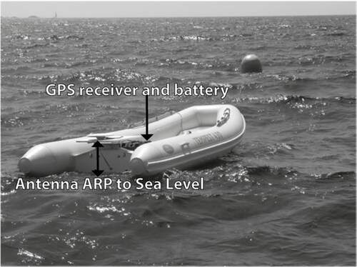
We have therefore designed a new system based on a small zodiac (∼2 m length) integrating both the antenna and the receiver (Figure 1). Such a system minimizes the loss of lock issue and allows relatively high-speed operation between different comparison points (>7 knots) in order to use the same system both for doing the altimeter calibration at a specific comparison point and for mapping large areas. Unfortunately, tests at different speeds showed a strong dependence of the waterline to velocity and sea state which was difficult to model at 1-centimer accuracy; Thus, the SSH are only retained when the zodiac is in “static” conditions, the rest of the GNSS data being only used for maintaining the ambiguity sets in GNSS processing.

Figure 1. Zodiac boat used as GNSS-based sea level measurement system since 2012. GNSS receiver is on-board and connected to the antenna located at the rear.

At our request, the Technical Division (DT) of CNRS/INSU (Division Technique de l’Institut National des Sciences de l’Univers of the CNRS) has explored another approach which consists of a GNSS platform that may be towed at significant speed (∼10 knots) in order to undertake sea surface mapping over relatively large areas. The basic idea is to force the antenna reference point to be on the sea surface, by putting a GNSS antenna on a deformable floating carpet (a concept named CalNaGeo, Figure 2; in French CalNaGeo stands for “Calibration avec Nappe Géodésique”). Here, we present the results obtained during an experiment which was carried out at the Senetosa site on 2015/06/18 in order to estimate the stability of the waterline as a function of the velocity. Note that to a lesser extent, the sea state may also have an impact but was not studied here because no major change in sea state was encountered during the experiment. This experiment was also designed to map the local ‘‘geoid’’ and then compare the slope to the existing geoid computed by Bonnefond et al. (2003) using the Catamaran in 1999. This study follows the first validation which was realized in 2010 using a GPS buoy as reported by Bonnefond et al. 2013. In this paper, Section “Instrumentation” focuses on the description of the instrument while Section “Methodology” describes the experiment’s methodology. Section “Results” presents and discusses the results.

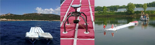
Figure 2. Photos of CalNaGeo. Left: for offshore use (open ocean; two inflatable boats) during this experiment (the GNSS-Zodiac can be seen on the right in the background and the lighthouse, where the reference receiver is, on the left in the background). Right: for inshore use (coastal ocean, lakes, rivers; one inflatable boat) during a campaign on the Seine river, France in June 2017. Middle: zoom on the gimbal system (photo from another experiment).

Instrumentation

Gnss-Zodiac

At both locations of the Corsica calibration site (Senetosa and Ajaccio), in addition to the coastal tide gauges, there are open-ocean comparison points for repeated deployments of GNSS-based sea level measurement systems (Bonnefond et al. 2003, 2013). A major change has been implemented since 2012: the traditional waverider buoy was replaced by a Zodiac (termed GNSS-Zodiac hereon and abbreviated “zodi”; see Figure 1) for both calibration sites. The main reason was that a waverider buoy cannot be towed by a boat. As a consequence, handling (from sea to boat and vice versa) leads to losses of the GNSS signal that affect the ambiguity resolution in the data processing. Moreover, in the case of harsh sea-states, significant tilts of the buoy and/or water over the antenna may also lead to loss of lock (Bonnefond, Haines, and Watson 2011; Watson et al. 2011) or systematic error related to the antenna not being horizontal (Zhou et al. 2020). The use of the GNSS-Zodiac instead of the previous buoy avoided these problems and thus allowed us to determine Sea Surface Heights (SSH) continuously between 1 and 50 Hz. On-board, the GNSS receiver (Trimble NetRS) is connected to the antenna (Trimble Zephyr Geodetic) located at the rear. The height from the antenna ARP down to the sea level (47 cm) is measured regularly with a rule in calm sea conditions in order to control and change the value in the processing if necessary: the stability of this reference from all the measurements performed so far was estimated to be better than 5 mm.

CalNaGeo

An important challenge with the floating GNSS systems is to continuously estimate or monitor the GNSS antenna height above the water level which varies with the load and speed of the platform, as well as the water density. To overcome this situation, the French DT-INSU/CNRS has developed a deformable floating towed carpet named CalNaGeo. Inspired by the capacity of floating seaweed to “hug” the sea surface, this system consists of a GNSS antenna mounted on a deformable floating sheet towed by a boat, ensuring good coupling with the sea surface and ideally, a constant antenna height above the water.

The CalNaGeo GNSS system can be towed for SSH mapping at high speed (up to 10 kn) and in rough seas (the original design was made for the Southern Ocean sea conditions). The system consists of a geodetic GNSS antenna (Trimble Zephyr Rugged) mounted on a soft shell that follows the sea surface as seaweed follows swell and waves, ensuring a constant antenna height above the sea surface. The length of the carpet and the inflatable boats at the front (∼10 m in total) has been chosen to mechanically smooth sea state effects at short wavelength. The antenna is mounted on a double gimbal tied to the carpet to keep it quasi-horizontal, and then guarantee good signal quality and to limit GNSS signal outages and loss of lock. A counterbalance with rubber bands is placed below the gimbal to prevent resonance (Figure 2, middle); the type and tension of the rubber bands are empirically chosen as a function of the sea-state conditions. The antenna is cabled to the receiver (Trimble NetR9) powered by batteries and are both installed in one inflatable boat at the front of the soft shells (the number of inflatable boats depends on the application, e.g., open ocean versus river and lake/seashore; Figure 2, left and right panels respectively). The orientation of the antenna is measured relative to the direction of the length of the carpet to enable the determination of the absolute orientation with respect to an Earth fixed frame: this parameter is not used for the moment but improvements are foreseen to include it in the processing in order to limit the phase wind-up effects (e.g., Zhou et al. 2020). A telecommunication system (using a Xbee module and NMEA standards) enables operators to check the status of GNSS acquisition (e.g., number of satellites and CalNaGeo’s location) within a distance of 1-2 km. The whole CalNaGeo platform (soft cell structure and inflatable boats) can be towed by a ship at up to 10 knots at a distance of several hundreds of meters to reduce the effect of the boat’s wake. For this experiment and considering the length of the wake of the boat used for towing CalNaGeo, the chosen distance was ∼100 m.

The CalNaGeo system can be used for in situ SSH mapping useful for altimetry validation, marine geoid measurement and wave monitoring, with recording rates up to 50 Hz. This design has been tested under various conditions: In the open ocean (Kerguelen, offshore California and in Noumea lagoon), in the coastal zone (Bangladesh, Pertuis Charentais and Corsica) and in rivers (Seine, Gironde in France and Maroni in French Guyana). The CalNaGeo system will be abbreviated “cngh” hereon (particularly in the Tables and Figures). The nominal height from the antenna ARP down to the sea level measured under static (calm) conditions, is estimated to be 44.5 ± 0.1 cm, as determined by multiple measurements with a rule; this rule is temporally installed on the gimbal for these measurements and pictures are taken to measure the position of the water which flushes the base of the carpet (white seams on Figure 2, center).

Methodology

For the 1999 campaign (Bonnefond et al. 2003), a catamaran had been built using 2 windsurfer boards connected by a metallic structure on which antennas were fixed. This design had been chosen to limit hydrodynamic effects that change the buoyancy location as a function of velocity. However, at this time, no dedicated study had been performed to quantify the stability of the waterline as a function of velocity. As a consequence, to avoid such speed-dependent sea-height variations, only data acquired at speeds between 3 m/s and 3.7 m/s had been kept in the analysis. The concept of our newly developed instrument (CalNaGeo) is to ensure that the height of the GNSS antenna above water is almost constant whatever the velocity and our experiment has been designed to evaluate this stability. Thanks to such a stability, CalNaGeo data can be used without any thresholds nor corrections involving the velocity parameters. Given some other effects that are difficult to quantify (for example, change in antenna position when surfing on larger waves), we continue to recommend maintaining a constant velocity during SSH mapping exercises. The nominal speed is 8 knots which is strongly dependent on sea state conditions. During the SSH mapping phase of this experiment (see Section “Off shore phase”) the velocity was set to be almost constant (∼8 ± 0.6 knots).

Description of the experiment’s phases

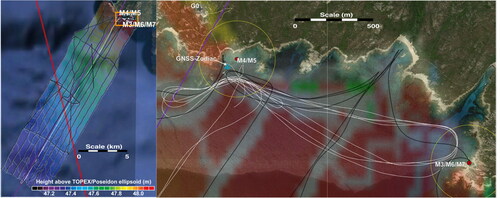
The experiment held on 2015/06/18 was designed with two objectives in mind: to estimate the stability of the CalNaGeo waterline as a function of the velocity in the vicinity of the tide gauges (near shore phase, see Figure 3 right panel), and to re-measure the geoid slope along the center of the map from Bonnefond et al. (2003) (off shore phase, Figure 3 left panel). During all of the experiment, the GNSS-Zodiac remained operational and anchored at the same location (see Figure 3 right panel).

Figure 3. Left: Full experiment area (orange rectangle corresponds to the zoom at right). Right: Zoom on the area where tide gauges are located. Purple and Red lines are the Jason and Sentinel-3A ground tracks respectively. Colored contour map and black lines from GPS measurements during the 1999 Catamaran experiment (Bonnefond et al. 2003). White lines from CalNaGeo GPS measurements during the 2015 experiment (this study). Red dots for tide gauges (M3 and M5 in this study). Yellow circles mark the 250 m distance to compare SSH from GNSS and tide gauges. The GNSS-Zodiac was anchored at about 90 m Westward from the M5 tide gauge (blue anchor on the Figure). Grey cross for the permanent GNSS receiver (G0 in the lighthouse area, upper left in right hand panel).

Near shore phase

During this phase, we made several passes close to the tide gauges (mainly the M5 tide gauge, see Figure 3 right panel) within a 250 m distance and at different velocities, incrementally from 0 up to 6 m/s (see white lines in Figure 3, right) the goal being to estimate the stability of the waterline as a function of the velocity (see Section “Effect of velocity on the SSH measurements”). Moreover, during two periods of time (before and after the offshore survey, see orange lines in Figure 4) we also made static measurements (not towed) within 250 m from M5 tide gauge: The first one lasts from 6h20 to 6h48 and the second one from 9h42 to 10h52. This was designed to estimate the quality of the GPS solutions by comparing the CalNaGeo and GNSS-Zodiac SSH, respectively, to both SSH time series from the M3 and M5 tide gauges. It also allowed us to monitor any systematic changes (see Section “Static period”) of the GPS solutions (for differential processing) due to the increase of the distance from the permanent GPS receiver (G0 in Figure 3, right panel) during the offshore phase that may change the ambiguity set compared to the one at short distance.

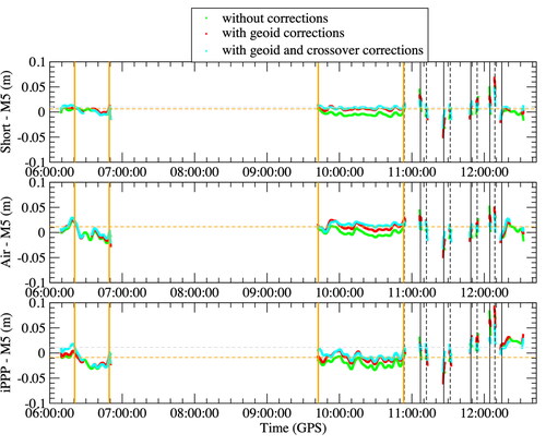
Figure 4. SSH differences with M5 tide gauge when within 250 m (cngh – M5) as a function of time without corrections (green crosses, Table 6), with geoid corrections (red crosses, see Table S5 under the Section “Additional tables and figures” in the supplemetary file) and with both geoid and weighted and smoothed crossovers corrections (cyan crosses, Table 7): top, middle and bottom for “Short”, “Air” and “iPPP” GPS solutions respectively. Dashed vertical black lines correspond to Eastward passes close to M5. Solid vertical black lines correspond to Westward passes close to M5. Orange vertical lines correspond to beginning and end of the phases when cngh was static (close to M5 and zodi, see Tables 3–5). The horizontal dashed lines correspond to the mean for static periods (orange, inside vertical orange lines) and periods with velocity (grey, outside vertical orange lines) for the solutions with both geoid and weighted and smoothed crossovers corrections (cyan crosses).

Off shore phase

This phase was designed to measure the geoid slope along the centerline of the marine geoid surveyed in the 1999 Catamaran experiment, for comparison purposes. CalNaGeo was towed from the M5 tide gauge location up to the end of the 1999 “geoid” map along its centerline (see white lines in Figure 3, left panel) and back to initial location at constant speed of ∼4 ± 0.3 m/s (∼8 knots). During the 1h27 outbound and 1h23 inbound survey (both completed between 6h50 to 9h40 UTC) the tracks were very close (∼10 m) in order to compare the stability of the GPS solutions.

GPS processing

Even if the two systems (CalNaGeo and Zodiac-GNSS) were equipped with antennas and receivers able to record the main constellations (GPS, Galileo, GLONASS) we only retain, for this study, the GPS data for all the computations because Galileo constellation was not complete at this time and GLONASS precision was perceived to be worse than GPS. Other studies including a multi-constellation processing strategy will be undertaken in the near future. The GPS processing has been realized for both survey phases using two main approaches: (i) a differential approach with G0 as reference receiver (see Figure 3, right panel) using TRACK software version 1.31 (TRACK is part of the GAMIT package to compute kinematic GPS; Herring 2003) and (ii) a Precise Point Positioning approach with integer ambiguity fixing (iPPP) using GINS software version 20.2 (Laurichesse et al. 2009). For both processing approaches, orbit and clock parameters come from the recent reprocessing relative to ITRF2014 reference frame. However, they are not available as a sp3 combined product (IGS) before 2017/01/29. Because TRACK is using sp3 files, we used the reprocessed JPL14 sp3 files relative to ITRF2014 reference frame (Bertiger et al. 2020). With GINS, we used its own format (GRG repro3 also relative to ITRF2014 reference frame, https://igsac-cnes.cls.fr/html/products.html; Loyer et al. 2012). For the differential approach, however, the choice of the orbit and clock parameters has negligible impact given the short distance between the mobile and the reference receiver (submillimeter level when comparing solutions using IGS08 and JPL14 sets). For both differential and iPPP approaches the elevation mask has been set to 10° with no elevation weighting and GPS data were processed at 1 Hz. The coordinates of the reference receiver (G0, Figure 3 right panel) are set to a constant defined by Bonnefond et al. (2021) because the height velocity is statistically not different from 0. However, these values may be different from determination over shorter timescales (e.g., during this experiment) differentiating such signal from noise is still a challenge. To give an order of magnitude of such differences when compared to the reference coordinates used, the daily solutions for the whole time series have a standard deviation of 3.8 mm and differences up to 31.7 mm peak to peak. This may have an impact when comparing the absolute SSH determined from the differential or the iPPP approaches. This will be further discussed in the Results section. However, the potential absolute systematic error in the SSH is not of importance for mapping the sea surface because in the calibration process we only use the height differences to transfer the SSH from the altimetry locations up to the coastal tide gauges (see Bonnefond et al. 2021 for more details). We must note that such systematic errors also have a time-variable component which is difficult to quantify. For this experiment, we consider this time-variable systematic error to be negligible.

For the first approach (differential), the processing is based on differential GPS computations using two strategies in the TRACK suite for both GNSS-Zodiac and CalNaGeo. The first TRACK mode used is called “short mode” (named “Short” hereafter) and is using L1 + L2 for the search analysis (searching over ambiguity space and looking for the best choices) and then LC (ionosphere free linear combination) to generate position estimates (retaining floating values of ambiguities from non-integer estimates). The second TRACK mode used is called “Air mode” (named “Air” hereafter) and is using LC for the search analysis (searching over ambiguity space looking for the best choices) that allows to account for perturbation to the cycle count due to ionospheric effects; LC is then used identically to generate position estimates. The first mode (“Short”) attempts to resolve ambiguities assuming the data differencing has attenuated common errors from the fixed and mobile receivers (orbit, clocks, tropospheric and ionospheric corrections) while the latter one (“Air”) acknowledges that this assumption no longer holds given the increased separation between the reference and mobile sites: this separation varies from ∼400 m (close to the tide gauge) up to ∼20 km, at the extremity of the region mapped (Figure 3 left panel). In both modes used in TRACK, the tropospheric correction is considered the same for the mobile and fixed receivers (i.e., it is not parameterized in the solution).

The second approach (absolute) is based on Precise Point Positioning with integer ambiguity resolution (named “iPPP” hereafter). Such processing needs to correct for Solid Earth tides (Petit and Luzum 2010) and Ocean Tide Loading (FES2014; Lyard et al. 2020). In a PPP approach, the tropospheric delay needs to be estimated together with the positions. The model used by GINS is based on Global Pressure and Temperature (GPT; Lagler et al. 2013) for the nominal values of the dry troposphere correction; the wet part is estimated from GPS data using the Vienna Mapping Functions (VMF; Boehm, Werl, and Schuh 2006) and the corrections applied to the observations are continuous (piece-wise linear) without adding any constraint nor tropospheric gradient. Because of the well-known correlation between the tropospheric delay and height, we have tried different temporal estimation of the wet delay parameter in order to estimate the best compromise: 1, 2, 12, 24, or 96 delays per day. Results (see Table S1 for GNSS-Zodiac and Table S2 for CalNaGeo under the Section “Additional tables and figures” in the supplemetary file) show that the optimal sampling is 12 delays per day (1 every 2 hours), minimizing the standard deviation of the differences with SSH from tide gauges (serving as reference) while trying to estimate changes in the troposphere during the experiment’s duration (∼6h30) that cannot be achieved using the 1 or 2 delays per day, even if they give slightly better statistics. This choice also minimizes the mean of those differences that reflects the transfer from the tropospheric correction to the SSH which correlation increases for higher rate sampling (24 and 96 delays per day).

Tide correction

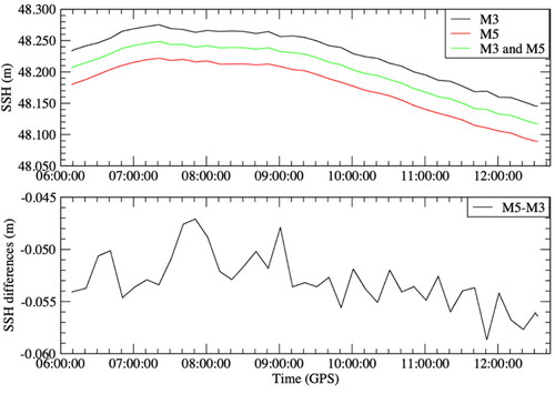
In order to compute crossover differences and the final “geoid” slope, the GPS SSH need to be corrected for the effect of ocean tides. The differential effects (between locations of CalNaGeo and tide gauges) of tides and atmospheric pressure must also be taken into account in the error budget. The magnitude of these effects depends not only on local conditions (for example, the shape of the coast, bathymetry), but also on the distance over which the SSH correction is transferred. These differential effects (tidal models and atmospheric pressure) are not used in this experiment because the estimated impact, even using high-resolution models, is at the level of a few millimeters over the considered area (Cancet et al. 2013). Thus, the corrections for ocean tide, inverted barometer and the high frequency wind and pressure response are not applied in this study. The tide correction has thus been performed using tide variations measured by the M3 and M5 tide gauges (see Figure 3, right panel). The tide gauges installed at the site are pressure-based gauges and were developed by DT-INSU/CNRS (see Bonnefond et al. 2021 for more details) and the atmospheric pressure to correct the raw measurements are from the weather station located close to the GNSS receiver (G0) at the lighthouse (see Figure 3 right panel). Height differences between instantaneous SSH measured by the tide gauges every 10 min and GPS are interpolated at 1 Hz. Figure 5 presents the tidal signal as seen by M3, M5, the average of both (top) and the differences between them (bottom). Despite the small SSH difference between tide gauges (2.3 mm standard deviation) and most probably due to instrumental differences (quartz, electronics, ….), it has been chosen to use the average of M3 and M5 SSH in order to minimize local effects on tide gauges measurements. The mean of the differences is of −53.0 mm which is related to the geoid slope between M3 and M5 locations and was already measured at −58.1 mm by Bonnefond et al. (2003). This is also confirmed by the mean value of −56.4 mm which has been obtained from the period (2013/01/01-2020/12/31) using the most recent and precise tide gauges built by the DT-INSU (Bonnefond et al. 2021). In terms of slope, it represents ∼3 cm/km which is surprisingly close to the average signal over the whole area (∼4 cm/km) noting the difference is caused by the direction between M3 and M5 being slightly different than the direction of maximum slope in the region.

Figure 5. Top: SSH tidal signal (height above the TOPEX/Poseidon ellipsoid) for M3 tide gauge (black line), M5 tide gauge (red line) and average of M3 and M5 tide gauges (green line). Bottom: SSH differences between M3 and M5 tide gauges.

Geoid correction

The grid determined during the 1999 Catamaran experiment (Bonnefond et al. 2003) is bilinearly interpolated to correct the GPS SSH from CalNaGeo making them directly comparable with SSH from the tide gauge locations. This grid is used in the absolute altimeter calibration process applied since 1998 (Bonnefond et al. 2021) and was validated in Bonnefond et al. (2013).

Crossover correction

In order to avoid confusion with the standard crossover strategy used in altimetry, we must note here that our approach is based on searching for locations where CalNaGeo has sampled the same spatial location more than once - we continue to use the term crossover hereon. Raw crossovers differences (cyan crosses in Figure 6) between GPS filtered SSH have been determined using the following criteria: (i) a distance lower than 10 m (between two CalNaGeo locations, see orange crosses in Figure 6) and (ii) a time lag higher than 900 s to avoid too many crossovers during the static phases.

Figure 6. Examples of crossovers: raw GNSS positions at 1 Hz (orange line and crosses), raw SSH crossovers (cyan crosses) and averaged SSH crossovers from raw ones (purple diamonds, annotated values correspond to the averaged time difference). Left: One track crosses another one (main horizontal and vertical ticks every ∼10 m). Right: One track follows another one (main horizontal and vertical ticks every ∼100 m).

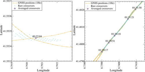
These criteria lead to a high number of candidate “raw crossovers” (cyan crosses in Figure 6), given that crossovers are not are not defined as single geometric points but have multiple realizations over a 10 m area that are not independent (one position on a track gives multiple crossovers with positions on other tracks); the location is the mean of the two positions used for forming the crossover. Crossover locations are also generated when tracks are aligned and don't cross orthogonally (e.g., Figure 6 left and right panels). This occurs frequently given the outbound and inbound track was within ∼10 m of each other. In order to minimize the impact on the statistics, mean crossovers (purple diamonds in Figure 6) have been computed from groups of raw SSH crossovers using the following criteria: (i) in case of a time gap is larger than 9 s between two consecutive raw crossovers, a new group is created and (ii) in case of the time lag difference for two consecutive raw crossovers is lower than 100 s (within a distance below 1000 m) the average is computed over a duration of 1 h; if the duration is larger than 1 h then several average points are created. This second criteria allows to group raw crossovers that have common time correlated errors (same time lag) and only retain long wavelength ones in terms of spatial (1000 m, close to the filtered SSH) and time sampling (1 h, which can be linked to GPS processing errors). The averaged standard deviation of each computed averaged crossover is ∼2 mm showing the coherency of the raw crossovers and the legitimacy to make mean crossovers. In this study, there were ∼3.7 10⁶ raw crossovers that are summarized by ∼320 mean crossovers (see Table 1). The distribution of the time lags is given in Figure 7 (bottom panel): ∼50% have time lags below 5000s and ∼86% for time lags below 10000 s.

Figure 7. SSH differences at crossovers as a function of time (top left) and as a function of time differences (top right), for “Short” (black crosses), “Air” (red diamonds) and “iPPP” (green circles) GNSS solutions. Bottom: histogram of the time differences (time lag) at crossovers.

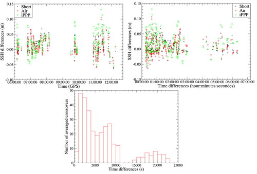
Table 1. SSH crossover differences for different processing strategies and tide corrections.

Tide correction / processing	Mean (mm)	Standard Deviation (mm)	Number
M3
Short	+10.6	24.4	321
Air	+7.6	23.6	321
iPPP	+17.1	30.7	317
M5
Short	+11.5	24.5	321
Air	+8.6	23.5	321
iPPP	+18.1	31.3	317
M3&M5
Short	+11.1	24.4	321
Air	+8.1	23.5	321
iPPP	+17.6	31.0	317

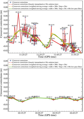
In the following, the averaged crossover differences will be used to correct the GPS SSH for remaining errors in the GPS processing. GPS systematic error from orbits/clocks/geometry but also antenna’s Phase Center Variations will express as a complex function of time. The bigger the time lag in the crossover, the bigger the potential for GPS systematic effects not to cancel. If the time lag is very short, then GPS systematic effects from these sources will largely cancel. The second criteria (described previously) for grouping raw crossovers that have common time correlated errors attenuates the long temporal wavelength component mostly caused by GPS systematic effects. For short temporal wavelength, we thus developed a weighted model and smoothing to downweigh the contribution of crossovers with short time lag. Using a simple linear interpolation (red crosses, Figure 6 top panel) between crossovers leads to adding noise in the GPS solutions at high frequency. This is particularly the case for the period mentioned in the next section (from ∼10h50 to ∼12h20, see Figure 4), due to lots of turns and disturbances from the boat wake. We thus smoothed the mean crossover differences in two steps: first using a weighted (normalized time difference) moving average (orange crosses: width = 300 s/Step = 30 s) and second by smoothing them with a 60 s low-pass filter (green crosses; Vondrak 1977). Results of the 2 methods, “simple linear interpolation” and “weighted and smoothed”, are given in Section “Additional tables and figures” (Tables S5 and S6, respectively). Even if the linear interpolation (red crosses, Figure 8 bottom panel) is equivalent to the two-step smoothing (green crosses), in the case of more regularly spaced crossovers, there is an improvement in terms of the variability (as described by the standard deviation) thanks to “weighted and smoothed” approach (see Figure 8 top panel). The latter approach has been adopted in the following analysis.

Figure 8. Averaged crossover corrections as a function of time (blue crosses), linearly interpolated at 1 Hz solution time (red dots), with a weighted (normalized time difference) moving average (width = 300 s/Step = 30 s, orange dots) and finally smoothed by a 60 s low-pass filter (green dots). Time differences are given in annotated values. Top: period with high density of crossovers. Right: period with low density of crossovers.

Results

GPS processing comparisons

All GPS SSH (whatever the velocity) have been filtered using Vondrak filter (Vondrak 1977) prior to any other processing (tide correction, crossover…). The advantage of such a filter, compared for example to a boxcar average, lies in its very sharp response curve that reduces the amplitude of artificial short period signals generally generated by low-pass filters. Moreover, the Vondrak filter allows the use of data series with gaps. Filtering has been applied in the time domain using a low-pass with a 300 s cutoff period. In the space domain, this filter retains signals in SSH with wavelengths higher than approximately 1200 m (at a speed of 4 m/s) allowing to remove signals from swells and waves notably. All the statistics presented in this study are based on filtered SSH.

Table 2 and Figure 9 illustrate the differences between the different solutions for both GNSS-Zodiac and CalNaGeo. Because the GNSS-Zodiac was anchored during the whole experiment (see Figure 3 right panel), it is used as reference for comparing the solutions. The lowest standard deviation is obtained for GNSS-Zodiac “Air - Short” differences; it illustrates that, as expected, including potential differential effects between reference and mobile receivers at such very small distance (less than 400 m from the G0 reference receiver) with the “Air” mode leads to a noisier SSH. The standard deviation for GNSS-Zodiac “iPPP - Short” differences is larger than using “Air - Short”; it illustrates that even with the recent improvements in the orbit and clock parameters, the iPPP processing is of lower precision than short baseline differential processing. When looking at the differences for CalNaGeo, the standard deviation increases compared to the GNSS-Zodiac due to the displacement of the CalNaGeo platform away from the reference site as conditions changed making ambiguity resolution more challenging (e.g., change in geometric configuration, small tilts of the antenna, …). The highest standard deviation is unsurprisingly observed in the CalNaGeo “iPPP - Short” differences, mainly during the offshore period but especially for the farthest distance from the reference receiver (Figure 9 bottom, from 7h50 to 8h50 with a distance from ∼14 to ∼20 km). This was expected given the known limitations of not forming an ionospheric free observable for ambiguity resolution over a few km.

Figure 9 SSH differences for zodi (top) and cngh (bottom): “Air - Short” (black lines), “iPPP - Short” (red lines) and “iPPP - Air” (green lines) G solutions respectively. Horizontal lines correspond to the mean of each set of differences (see Table 2).

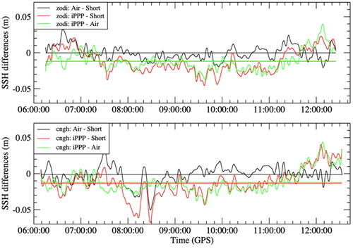
Table 2. SSH differences statistics without any outliers’ removal for the different processing strategies and type of instruments and for all epochs (1 Hz).

Type of differences / instruments	Mean (mm)	Standard Deviation (mm)	Number (1Hz)
Air - Short / zodi	−0.2	9.8	22199
Air - Short / cngh	−1.3	12.2	23039
iPPP - Short / zodi	−12.0	15.8	22199
iPPP - Short / cngh	−13.5	18.7	23010
iPPP - Air / zodi	−11.8	13.3	22199
iPPP - Air / cngh	−12.2	15.3	23010

The mean of the differences provides an indication of the accuracy of the processing but we must note that other types of systematic errors can be common for both differential and PPP approaches (e.g., antennas phase center offsets and variation) and are canceled in the differences; Table 2 shows a ∼1 cm difference when comparing iPPP processing to the “Short” and “Air” relative processing solutions. This will be discussed more extensively in Section “Comparisons with tide gauges” but it illustrates the difficulty to achieve a centimetric accuracy notably for iPPP processing. In another study (not yet published), from comparisons with JPL Gipsy processing we also have such centimetric bias that is probably linked to some discrepancies in the orbit and clock parameters. Another source of systematic error can come from the coordinates (mainly the up component) of the reference receiver used in the differential approach. As previously said, it is set to a constant value (same as the one used in the calibration process, see Bonnefond et al. 2021) and the difference from a daily solution can be few tens of mm, compatible with mean differences shown in Table 2). Nevertheless, theses biases will not affect the final “geoid” survey because we are focusing on differences of heights (or slope).

Analysis of the SSH crossovers differences

Different GPS processing techniques and tide correction types were used; on the one hand standard deviations (Table 1) are very close regardless of the chosen tide correction (we retain the mean between M3 and M5), on the other hand, “Air” mode (see Section “GPS processing”) is probably the best compromise and shows the lower standard deviation.

Figure 7 (left panel) shows the crossover SSH differences as a function of the time of the first GPS measurement in the crossover. The period during which the stability of the waterline was tested at different velocities (from ∼10h50 to ∼12h20 UTC) appears to be noisier. This is probably due to the persistence of boat wake and to the GPS processing (lots of short turns that can create potential carrier phase wind-up error but also the velocity that makes the positioning more difficult to solve for). In addition, Figure 7 (right panel) shows the crossover SSH differences as a function of time differences. It illustrates that the time domain is well covered (see also Figure 7 bottom) avoiding some aliasing with dynamic signal(s) in the SSH that can occur if the time lag is always close to the same value and corresponds to any possible physical temporal signal: most of the time lags are below 3 hours (∼86%) and dynamic signals at this time scale are not well known but supposed to be of small amplitude (in constant weather conditions and it was the case during our experiment); The other group of time lags is between 3h50 and 6h20 and this area being dominated by M2 tide, no aliasing with remaining errors in this constituent should appear. Figures S4–S6 in Section “Additional tables and figures” give the geographical distribution of the SSH differences at crossovers respectively for the “Short”, “Air” and “iPPP” processing and show similar patterns that are probably linked to common GPS systematic errors.

Comparisons with tide gauges

Due to the difficulty to conduct long passes or static periods close to M3 (numerous outcropping underwater rocks), the number of measurements is thus very low, however, results are coherent with results from M5. The results in this section will focus on the SSH comparisons with M5 tide gauge measurements, but statistics for M3 can be found in Section “Additional tables and figures” (Tables S8–S12). All the statistics given for the SSH differences are from all the data without any outlier detection process undertaken.

Static period

The “static” periods are used to compare the GPS SSH without adding other effects (change of geometry, small tilts of the antenna, …) and also helps in the ambiguity fixing: The first one lasts from 6h20 to 6h48 (UTC) and the second one from 9h42 to 10h52 (UTC). Tables 3 and 4 present the cumulated statistics of the SSH differences with M5 when the distance from M5 lower than 250 m and the velocity is lower than 0.3 m/s (allowing to take into account a small velocity during slow horizontal drift of the mobile platforms due to currents and wind). For CalNaGeo, some data are outside these two periods because the two criteria (velocity and distance) were also reached. To be comparable, statistics of common data in time from both the GNSS-Zodiac and CalNaGeo mobile’s platforms are given in brackets; the mean reveals some biases with M5 tide gauge measurements. For the GNSS-Zodiac, the bias is close to −10 mm for both “Short” and “Air” processing techniques and raises up to −23.8 mm (larger by ∼14 mm from differential solutions) for “iPPP” processing. A similar increase (∼16 mm) is also seen for CalNaGeo; it is probably due to orbit and clocks inaccuracies that affects the Precise Point Positioning processing while canceled in the differential one. Differences between differential and PPP approaches may also come from the position of the reference receiver (as previously discussed), and thus illustrates the difficulty of guarantying an absolute SSH at the centimeter level. In addition, we found a bias of ∼6 mm between GNSS-Zodiac and CalNaGeo, illustrating the difficulty to define the absolute waterline at the few millimeter level.

Table 3. Statistics of SSH differences with M5 tide gauge (zodi – M5) within 250 m (velocity < 0.3 m/s). Values in brackets correspond to common data in time with cngh (see Table 4).

Type	Mean (mm)	Standard Deviation (mm)	Number of data	Mean Distance (m)
Short	−11.5 (-10.7)	4.7 (3.5)	20992 (5468)	93 (87)
Air	−12.2 (-8.2)	9.6 (10.7)	20992 (5463)	93 (87)
iPPP	−23.7 (-23.8)	13.8 (15.8)	21551 (5930)	92 (86)

Table 4. Statistics of SSH differences with M5 tide gauge (cngh – M5) within 250 m (velocity < 0.3 m/s). Values in brackets correspond to common data in time with zodi (see Table 3).

Type	Mean (mm)	Standard Deviation (mm)	Number of data	Mean Distance (m)
Short	−2.4 (-3.1)	4.4 (3.9)	5961 (5468)	115 (118)
Air	−1.2 (-2.1)	7.9 (7.1)	5957 (5463)	115 (118)
iPPP	−18.9 (-19.0)	11.1 (10.8)	5954 (5930)	115 (115)

For both the GNSS-Zodiac and CalNaGeo, the standard deviation of static SSH differences increases for the “Air” and even more for the “iPPP” processing compared to the “Short” one, illustrating that taking into account ionospheric and tropospheric effects at such very small distance (less than 400 m from G0 reference receiver) leads to a noisier SSH. However, the CalNaGeo standard deviation is generally lower whatever the processing showing that the double gimbal used for maintaining the antenna as horizontal as possible leads to an improvement in the data quality and homogeneity. In conclusion, the low level of standard deviation (15.8 mm for the worst case and 3.5 mm for the best one) reinforces the ability of GPS to enable high precision GPS-based sea level measurements.

Table 5 shows same statistics as Table 4 but after correcting the SSH with weighted and smoothed crossover corrections and with geoid corrections (see Sections “Crossover correction” and “Geoid correction” respectively). This allows us to estimate the final precision of the corrected SSH. Statistics are very comparable to the ones of Table 4, even if the numbers of data are not exactly the same; in fact, some of them are outside the 1999 Catamaran geoid grid (very close to the coast, notably during the first static period, see Figure S7 in Section “Additional tables and figures” in the supplemetary file). The statistics in brackets are from the two defined static periods (before and after the offshore survey) in order to better estimate any possible systematic errors in the GPS processing before applying the crossover correction. In terms of standard deviation, the first period is generally noisier whatever the processing (see also Figure 4). This may be due to a less optimal configuration of the constellation, but there is no clear indication from either the Dilution Of Precision (Figure S1 under the Section “Additional tables and figures” in the supplemetary file) nor the phase residuals (Figure S2 in Section “Additional tables and figures”) to confirm this hypothesis. The “Short” processing is by definition less impacted by such effect. Concerning the mean, the differences (“after” minus “before”) are +8.5 mm, +16.0 mm and +11.9 mm for respectively the “Short”, “Air” and “iPPP” processing. Because these differences are relatively larger than expected, we have investigated the possible impact of the geoid correction notably when it is estimated too close to the border of the grid (edge effects). From Table S3 (see Section “Additional tables and figures” in the supplemetary file), where the geoid corrections are not applied, the same differences (“after” minus “before”) now are +4.2 mm, +7.2 mm and +2.6 mm, which confirms our assumption that very close to the coast the geoid correction is probably not accurate enough: indeed, some parts of the locations covered by CalNaGeo during the static phases (white lines in Figure 3 right panel) was not covered by the Catamaran in 1999 (black lines in Figure 3 right panel). In conclusion, we can say that the GPS solutions do not show any significant drift during the offshore phase, at the level of few millimeters.

Table 5. Statistics of SSH differences with M5 tide gauge (cngh – M5) within 250 m (velocity < 0.3 m/s) with weighted and smoothed (see Section “Crossover correction”) crossover corrections (using M3&M5 tide correction, see Table 1) and with geoid corrections (see also Table S4 under the Section “Additional tables and figures” in under the supplemetary file). Values in brackets (separated by a “/”) are for the first and second period of static measurements respectively (see vertical orange lines in Figure 4).

Type	Mean (mm)	Standard Deviation (mm)	Number of data	Mean Distance (m)
Short	+6.5 (-0.2 / +8.3)	4.4 (4.8 / 1.8)	5549 (1261/ 4040)	115
Air	+11.8 (-0.7 / +15.3)	8.9 (8.9 / 4.1)	5545 (1260 / 4037)	115
iPPP	−7.8 (-17.9 / −6.0)	10.3 (11.0 / 6.2)	5530 (1651 / 4034)	115

Moving period

The other phases were performed towing CalNaGeo at different velocities, notably with several passes close to the M3 and M5 tide gauges. Table 6 presents the statistics of SSH differences obtained with M5 within 250 m for all velocities (including those with velocity below 0.3 m/s presented in Section “Static period”), while Table 7 presents the same statistics but after applying both the ‘‘weighted and smoothed crossover’’ and geoid corrections (see Section “Crossover correction” and “Geoid correction” respectively). Applying these corrections clearly improves the standard deviation of the SSH differences by several millimeters (notably for the iPPP processing), and even gives similar results to the one presented in the previous section when CalNaGeo was static (see Tables 4 and 5). This gives us confidence in using such corrections (crossovers notably) to reduce remaining errors in the GPS solutions.

Table 6. Statistics of SSH differences with M5 tide gauge (cngh – M5) within 250 m (for all velocities). Values in brackets correspond to common data in time with the ones with geoid correction (see Table 7 in this section and Table S5 under the Section “Additional tables and figures” in the supplemetary file).

Type	Mean (mm)	Standard Deviation (mm)	Number of data	Mean Distance (m)
Short	−0.7 (-0.9)	8.3 (8.7)	8697 (7665)	118 (126)
Air	+1.0 (+0.9)	10.4 (10.6)	8697 (7665)	118 (126)
iPPP	−10.9 (-13.1)	19.3 (17.7)	8685 (7634)	118 (125)

Table 7. Statistics of SSH differences with M5 tide gauge (cngh – M5) within 250 m (for all velocities) with weighted and smoothed (see Section “Crossover correction”) crossover corrections (using M3&M5 tide correction, see Table 2) and with geoid corrections.

Type	Mean (mm)	Standard Deviation (mm)	Number of data	Mean Distance (m)
Short	+7.2	6.0	7665	126
Air	+11.1	9.7	7665	126
iPPP	−3.4	12.9	7634	125

The statistics given in this section include the periods when CalNaGeo was almost static (velocity < 0.3 m/s) which implicitly leads to a reduced standard deviation. The following section will focus on data during which CalNaGeo was towed. For example, the standard deviation increases from 11.1 mm (velocity < 0.3 m/s, Table 4) to 25.6 mm (velocity > 0.3 m/s, Table 8) for iPPP (without any corrections). The effect of a potential change of the waterline leads to a standard deviation of 11.2 mm (linear behavior of +6.8 mm/(m/s), Section “Effect of velocity on the SSH measurements”) and thus an increase of ∼5 mm (root sum square) compared to the 11.1 mm in “static” condition. Thus, the main part of the increase is mainly due other effects of the velocity (GPS processing, interaction of CalNaGeo with waves and currents…).

Table 8. Linear trend of SSH differences with M5 tide gauge (cngh – M5) within 250 m as a function of velocity (from 0.3 to 6 m/s). Values in brackets from a linear regression based on a “robust” least absolute deviation method (ladfit.pro IDL routine). “±” is the formal error from the regression process.

	Mean (mm)	Standard Deviation (mm)	Bias @ 0 m/s (mm)	Slope (mm/(m/s))	Number of data
Short
No corrections	+3.5	16.0	−6.1 ± 0.7 (-2.9)	+3.7 ± 0.2 (+2.2)	1568
With geoid corrections	+7.4	16.2	−1.2 ± 0.8 (+3.2)	+3.2 ± 0.2 (+2.2)	1496
With geoid and crossovers corrections	+7.9	10.0	+4.2 ± 0.5 (+7.1)	+1.4 ± 0.2 (+0.8)	1496
Air
No corrections	+2.1	15.4	−6.2 ± 0.7 (-2.4)	+3.2 ± 0.2 (+2.0)	1570
With geoid corrections	+5.5	16.6	−2.3 ± 0.8 (-1.4)	+2.9 ± 0.3 (+3.1)	1498
With geoid and crossovers corrections	+5.7	10.5	+1.9 ± 0.5 (+1.8)	+1.4 ± 0.2 (+2.1)	1498
iPPP
No corrections	+3.9	25.6	−13.6 ± 1.1 (-16.8)	+6.8 ± 0.4 (6.8)	1563
With geoid corrections	+6.7	25.7	−11.9 ± 1.1 (-11.0)	+7.0 ± 0.4 (+5.1)	1491
With geoid and crossovers corrections	+6.7	13.8	−3.0 ± 0.6 (-1.1)	+3.7 ± 0.2 (+3.1)	1491

Effect of velocity on the SSH measurements

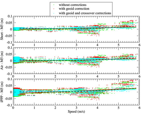
One of the main objectives of this experiment is to estimate the stability of the waterline of CalNaGeo as a function of velocity up to 6 m/s. But in order to minimize the impact of the “geoid” slope within the area, we first need to correct each individual 1 Hz GPS SSH relative to the tide gauge location from the “geoid” determined during the 1999 Catamaran experiment. The second step consists in using the crossovers SSH differences to correct for remaining errors in the GPS processing. Even if a boat squat (hydrodynamic sinkage) is physically more a quadratic function of speed, the difference between a quadratic and a linear fit is below 1 mm/(m/s) for the linear part and leads to ∼1 cm difference at the edges (for iPPP with all correction applied). We thus have chosen to only show the linear fit results given also the fact that a quadratic regression can be misfitted due to the lower density of data for high speed (5-6 m/s) where the linear and quadratic regression are diverging. However, black dash lines in Figure 10 illustrates these quadratic fits for the “geoid and weighted and smoothed crossovers corrections” sets. Table 8 summarizes the estimation of the slope of the SSH differences against the M5 tide gauge as a function of the velocity and Figure 10 illustrates the time series used. The standard deviation is clearly reduced when the SSH is corrected by the geoid and crossover corrections that improves the determination of the slope. As expected, because of the very close distance from the reference receiver, the “Short” solution gives the lower standard deviation that gives a very small dependence of SSH against velocity (1.4 ± 0.2 mm/(m/s)). After applying a standard linear regression the slope remains very close to the one determined with a “robust” least absolute deviation method (see numbers in brackets in Table 8), showing very few outliers. This is also the case for the “Air” solution with comparable values for the standard deviation and the slope. For the “iPPP” solution the standard deviation increases by ∼3 mm and the slope is also larger (3.7 ± 0.2 mm/(m/s)). The low formal errors (± in Table 8) suggests that the remaining uncertainty in the slope detection is not well considered in the noise model for the regression but the standard deviation of the slopes determined for all the processing approaches (with geoid and crossovers corrections) is 1.3 mm/(m/s) which gives an idea of the “real” uncertainty. In conclusion, it appears that the slope seems to be linked more to the quality of the GPS solution rather than to a physical lift-off effect; it is thus probably at a level below the mm/(m/s). The scatter increases for two parts of the velocity range (3-4 and 5-6 m/s), that can be seen in Figure 10, is clearly reduced when applying the geoid and crossovers corrections (cyan dots) but remains outside the uncertainty. We suspect that sometimes the CalNaGeo is surfing depending on the moving direction relative to the waves. However, it remains small (few centimeters locally) compared to the geoid signal to be mapped (several cm/km).

Figure 10. SSH differences with M5 tide gauge (cngh – M5) within 250 m as a function of velocity (from 0.3 to 6 m/s) without corrections (green crosses), with geoid corrections (red crosses) and with both geoid and weighted and smoothed crossovers corrections (cyan crosses) (corresponding color lines for the linear regressions, see values in Table 8): top, middle and bottom for “Short”, “Air” and “iPPP” GNSS solutions respectively. Black dash curves correspond to a quadratic fit for the “geoid and weighted and smoothed crossovers corrections” sets.

Differences with the 1999 “geoid” map

The second objective of this experiment was to measure the geoid slope along (Figure 3, left) the middle of the grid previously determined by Bonnefond et al. (2003). The GPS SSH are corrected from geoid slope using the 1999 Catamaran grid. Figure 11 shows these SSH as a function of the distance from M5 tide gauge with and without applying the weighted and smoothed crossovers corrections. From 2 km up to 20 km the standard deviations of the SSH differences are clearly reduced by applying the crossovers corrections whatever the processing approach used (Table 9). Figure 11 also shows a better consistency between the forward and outward journey. It illustrates that the strategy for crossover computation described in Section “Crossover correction” allows reducing the impact of GPS errors in the processing that affects the solutions at relatively long timescales (several hours). The higher standard deviation appears, as expected, with the “Short” processing because of the increasing distance from the reference receiver. The standard deviations of the “Air” and “iPPP” processing techniques, however, are at the same level (∼18 mm) and even lower for the latter; it illustrates that the Precise Point Positioning technique is now reaching the level of the classical differential approach. Table 9 also presents the estimation of the residual slope compared to the one determined in Bonnefond et al. (2003) that was estimated to be ∼40 mm/km in the direction of the centerline. This residual slope is negligible (below 1 mm/km, ∼2.5%) whatever the processing approach but the opposite sign for the “Short” processing again shows the effect of the increasing distance from the reference receiver. Some remaining patterns in Figure 11 (e.g., in the range of 6.5-10 km and 11-13 km), whatever the processing approach, may reflects some remaining errors in the 1999 ‘‘geoid’’ map but are very localized and have an amplitude generally less than 3 cm.

Figure 11. SSH differences with M5 tide gauge (cngh – M5) as a function of the distance to the coast (M5) without (black lines) or with (red lines) weighted and smoothed crossovers corrections (both corrected from geoid): top, middle and bottom for “Short”, “Air” and “iPPP” GNSS solutions respectively. Solid red lines and dashed black ones are for the linear regression for the remaining slope shown in Table 9 (note that being very close, the dashed black line is masked by the solid red one). Statistics (mean, standard deviation…) are given in Table 9.

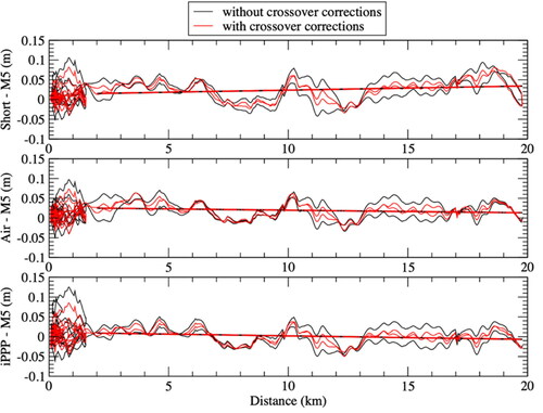
Table 9. Linear trend of SSH differences (cngh – M5) as a function distance to the coast (from 2 to 20 km). The poor agreement between 0 and 2 km has been excluded because it corresponds to the area where the stability of CalNaGeo waterline was tested and is not in the same along-track direction. “±” is the formal error from the regression process.

	Mean (mm)	Standard Deviation (mm)	Bias @ 0 km (mm)	Slope (mm/km)	Number of data
Short
No corrections	+24.7	29.6	13.1 ± 0.7	1.1 ± 0.1	9031
With crossovers corrections	+24.8	24.8	13.4 ± 0.6	1.0 ± 0.0	9031
Air
No corrections	+19.0	22.9	+26.1 ± 0.6	−0.6 ± 0.0	9031
With crossovers corrections	+19.1	18.1	+26.4 ± 0.4	−0.7 ± 0.0	9031
iPPP
No corrections	+12.4	22.6	+10.9 ± 0.5	−0.9 ± 0.0	9030
With crossovers corrections	+11.9	17.6	+10.7 ± 0.4	−0.9 ± 0.0	9030

Conclusions

In this study, we have demonstrated the capability of CalNaGeo to map the sea surface with a high accuracy and precision. In order to minimize the impact of remaining errors in the GPS solutions we have used the SSH crossovers to correct the SSH. Results show that the standard deviations of the SSH differences with tide gauge measurements are improved by several millimeters (Table 5 compared to Table 6) without significant changes of the mean (Table 5 compared to Table S7 under the Section “Additional tables and figures” in the supplemetary file).

In view of future activities, it was very important to assess the stability of the waterline whatever the velocity at which it is towed. The results (Table 8) show that the effect is probably no greater than 1 mm/(m/s) taking into account the remaining noise of the GPS solutions. Moreover, the absolute SSH do not exhibit a significant different bias when compared to the tide gauges with or without velocity (e.g., for iPPP processing,-3.4 mm in Table 7 and −7.8 mm in Table 5 respectively). These results are in good agreement with the ones presented in Chupin et al. (2020) and validate their study. Other effects (e.g., sea state, long swell, boat wake) can also affect the height of the waterline and are difficult to assess but filtering the data with a low-pass filter (here 300 s/1200 m cutoff) minimizes the impact. However, such effects can also have temporal changes at time scales greater than the filtering cutoff and can possibly impact the sea surface slope. This can notably be the case for larger study areas and for regions where the ocean dynamics are stronger. We unfortunately haven’t been able to identify such effects during our experiment because of the relatively small area covered where tides and ocean dynamics are small and well modeled. However, this study was mainly focused on the stability of CalNaGeo waterline as a function of velocity on relatively calm sea conditions. Additional effects can arise with different sea state conditions and slightly affect this stability but the length of the carpet has been designed to mechanically smooth these as much as possible. Other experiments have been conducted with CalNaGeo in different regions of the ocean (e.g., around Kerguelen island with SWH up to several meters, offshore California) and dedicated papers will try to better study all the possible impacts.

Given, this stability of the waterline, CalNaGeo has been used to determine the “geoid” slope along the centerline of the one determined during the 1999 Catamaran experiment. Results (Table 9) show that the measured residual slope is negligible (below 1 mm/km) validating also the SSH map used in the calibration process since 1998 (Bonnefond et al. 2021). CalNaGeo is thus able to measure slopes with a precision below 1-µrad, allowing the derivation high resolution geoid map even for wavelength of a few kilometers; however, some patterns over kilometer-length scales (see Figure 11) remain that are difficult to identify as real geoid undulations that would not have been present (or in error) in the previous SSH mapping. A 1-μrad error in slope translates into an approximately 1-mGal error in gravity (Sandwell et al. 2006; Sandwell et al. 2019). Translated into seamounts features, 1 µrad corresponds to a sea mount height of 1 km with a radius of 2.5 km. Such a precision is expected with SWOT measurements (Surface Water and Ocean Topography mission to be launched end of 2022) while current Ku-band altimetry is limited to ∼3.2 µrad (1.5 km height and 3.75 km radius) and only if localized under a satellite ground track. Recent improvements have been realized with the Ka-band onboard SARAL/AltiKa allowing to resolved small (700–1400 m tall) seamounts (Smith 2015).

Last but not least, we have investigated the impact of the GNSS processing using two different approaches and software. All the results show that the iPPP processing is now at the level of classical differential processing and probably better as the distance from the coast increases (and hence far from any coastal reference receivers). iPPP processing in addition to CalNaGeo offers a great opportunity to handle future experiments far from the coast, therefore from any reference receiver, even in open ocean conditions. Adding other GNSS constellations (e.g., Galileo) will most probably improves the precision and stability of the solutions and will be investigated in another dedicated study.

Acknowledgements

This study has been conducted and financed thanks to Centre National d’Etudes Spatiales (CNES), Centre National de la Recherche Scientifique (CNRS), and French Ministry of Research. This work has also received technical support from CNRS UAR855, INSU Technical Division. Special thanks to Claude Gaillemin who takes care of all the instruments at Cape Senetosa since 1998 and performs the deployments of the GNSS-based systems for sea level measurements.

Data availability statement

The data that support the findings of this study are available from the corresponding author [PB], upon reasonable request.

Additional information

Funding

This work was supported by Centre National d’Etudes Spatiales.

References

- Bertiger, W., Y. Bar-Sever, A. Dorsey, B. Haines, N. Harvey, D. Hemberger, M. Heflin, W. Lu, M. Miller, A. W. Moore, et al. 2020. Gipsyx/rtgx, a new tool set for space geodetic operations and research. Advances in Space Research 66 (3):469–89.
- Boehm, J., B. Werl, and H. Schuh. 2006. Troposphere mapping functions for GPS and very long baseline interferometry from European Centre for Medium-Range Weather Forecasts operational analysis data. Journal of Geophysical Research: Solid Earth 111 (B2).
- Bonnefond, P., B. Haines, and C. Watson. 2011. In situ calibration and validation: A link from coastal to open‐ocean altimetry. In Coastal Altimetry, ed. S. Vignudelli, A. Kostianoy, P. Cipollini, J. Benveniste, 259–96, Chapter 11. Berlin, Heidelberg: Springer. https://doi.org/https://doi.org/10.1007/978-3-642-12796-0_11
- Bonnefond, P., P. Exertier, O. Laurain, P. Thibaut, and F. Mercier. 2013. GPS-based sea level measurements to help the characterization of land contamination in coastal areas. Advances in Space Research 51 (8):1383–99.
- Bonnefond, P., P. Exertier, O. Laurain, T. Guinle, and P. Féménias. 2021. Corsica: A 20-Yr multi-mission absolute altimeter calibration site. Advances in Space Research 68 (2):1171–86. https://doi.org/https://doi.org/10.1016/j.asr.2019.09.049
- Bonnefond, P., P. Exertier, O. Laurain, Y. Menard, A. Orsoni, E. Jeansou, B. Haines, D. Kubitschek, and G. Born. 2003. Leveling Sea Surface using a GPS catamaran, Special Issue on Jason-1 Calibration/Validation, Part 1. Marine Geodesy 26 (3–4):319–34.
- Born, G. H., M. E. Parke, P. Axelrad, K. L. Gold, J. Johnson, K. W. Key, D. G. Kubitschek, and E. J. Christensen. 1994. Calibration of the TOPEX altimeter using a GPS buoy. Journal of Geophysical Research 99 (C12):24517–26.
- Bouin, M.-N., V. Ballu, S. Calmant, and B. Pelletier. 2009. Improving resolution and accuracy of mean sea surface from kinematic GPS, Vanuatu subduction zone. Journal of Geodesy 83 (11):1017–30. doi:https://doi.org/10.1007/s00190-009-0320-7.
- Bouin, M.-N., V. Ballu, S. Calmant, J.-M. Boré, E. Folcher, and J. Ammann. 2009. A kinematic GPS methodology for sea surface mapping, Vanuatu. Journal of Geodesy 83 (12):1203–17. doi:https://doi.org/10.1007/s00190-009-0338-x.
- Cancet, M., S. Bijac, J. Chimot, P. Bonnefond, E. Jeansou, O. Laurain, F. Lyard, E. Bronner, and P. Féménias. 2013. Regional in situ validation of satellite altimeters: Calibration and cross-calibration results at the Corsican sites. Advances in Space Research 51 (8):1400–17.
- Chupin, C., V. Ballu, L. Testut, Y.-T. Tranchant, M. Calzas, E. Poirier, T. Coulombier, O. Laurain, and P. Bonnefond. 2020. Mapping sea surface height using new concepts of kinematic GNSS instruments. Remote Sensing 12 (16):2656. https://doi.org/https://doi.org/10.3390/rs12162656.
- Clarke, J. E. H., P. Dare, J. Beaudoin, and J. Bartlett. 2005. A stable vertical reference for bathymetric surveying and tidal analysis in the high Arctic. In U.S. Hydrographic Conference. http://www.omg.unb.ca/orig/omg/papers/JHC_ushc2005.pdf.
- Crétaux, J.-F., M. Bergé-Nguyen, S. Calmant, V. V. Romanovski, B. Meyssignac, F. Perosanz, S. Tashbaeva, A. Arsen, F. Fund, N. Martignago, et al. 2013. Calibration of Envisat radar altimeter over the Lake Issykkul. Advances in Space Research 51 (8):1523–41.
- Crétaux, J.-F., S. Calmant, V. Romanovski, F. Perosanz, S. Tashbaeva, P. Bonnefond, D. Moreira, C. K. Shum, F. Nino, M. Bergé-Nguyen, et al. 2011. Absolute calibration of Jason radar altimeters from GPS kinematic campaigns over Lake Issykkul. Marine Geodesy 34 (3–4):291–318.
- Haines, B., S. D. Desai, D. Kubitschek, and R. R. Leben. 2021. A brief history of the Harvest experiment: 1989–2019. Advances in Space Research 68 (2):1161–70.
- Herring, T. A. 2003. GLOBK: Global Kalman filter VLBI and GPS analysis program Version 10.1. Internal Memorandum, Massachusetts Institute of Technology, Cambridge. http://www-gpsg.mit.edu/∼simon/gtgk/GLOBK.pdf
- Lagler, K., M. Schindelegger, J. Böhm, H. Krásná, and T. Nilsson. 2013. GPT2: Empirical slant delay model for radio space geodetic techniques. Geophysical Research Letters 40 (6):1069–73.
- Laurichesse, D., F. Mercier, J.-P. Berthias, P. Broca, and L. Cerri. 2009. Integer ambiguity resolution on undifferenced GPS phase measurements and its application to PPP and satellite precise orbit determination. Navigation 56 (2):135–49.
- Loyer, S., F. Perosanz, F. Mercier, H. Capdeville, and J.-C. Marty. 2012. Zero-difference GPS ambiguity resolution at CNES–CLS IGS analysis center. Journal of Geodesy 86 (11):991–1003.
- Lyard, F. H., D. J. Allain, M. Cancet, L. Carrère, and N. Picot. 2021. FES2014 global ocean tide atlas: design and performance. Ocean Science 17 (3):615–49. doi:https://doi.org/10.5194/os-17-615-2021.
- Martinez-Benjamin, J. J., M. Martinez-Garcia, S. G. Lopez, A. N. Andres, F. B. Pozuelo, M. E. Infantes, J. Lopez-Marco, J. M. Davila, J. G. Pasquin, C. G. Silva, et al. 2004. Ibiza absolute calibration experiment: Survey and preliminary results. Marine Geodesy 27 (3–4):657–81.
- Mertikas, S. P., A. Daskalakis, I. N. Tziavos, O. B. Andersen, G. S. Vergos, A. Tripolitsiotis, V. Zervakis, X. Frantzis, and P. Partsinevelos. 2013. Altimetry, bathymetry and geoid variations at the Gavdos permanent Cal/Val facility. Advances in Space Research 51 (8):1418–37.
- Petit, G., and B. Luzum, eds. 2010. IERS conventions. (IERS Technical Note; 36) Frankfurt am Main: Verlag des Bundesamts für Kartographie und Geodäsie, 179 pp.
- Roggenbuck, O., and J. Reinking. 2019. Sea surface heights retrieval from ship-based measurements assisted by GNSS signal reflections. Marine Geodesy 42 (1):1–24.
- Roggenbuck, O., J. Reinking, and A. Härting. 2014. Oceanwide precise determination of sea surface height from in-situ measurements on cargo ships. Marine Geodesy 37 (1):77–96.
- Sandwell, D. T., H. Harper, B. Tozer, and W. H. Smith. 2021. Gravity field recovery from geodetic altimeter missions. Advances in Space Research 68 (2):1059–72. doi:https://doi.org/10.1016/j.asr.2019.09.011.
- Sandwell, D. T., W. H. F. Smith, S. Gille, E. Kappel, S. Jayne, K. Soofi, B. Coakley, and L. Geli. 2006. Bathymetry from space: Rationale and requirements for a new, high-resolution altimetric mission. Comptes Rendus Geoscience 338 (14–15):1049–62.
- Smith, W. H. F. 2015. Resolution of seamount geoid anomalies achieved by the SARAL/AltiKa and Envisat RA2 satellite radar altimeters. Marine Geodesy 38 (sup1):644–71.
- Testut, L., M. Calzas, C. Drezen, A. Guillot, P. Bonnefond, O. Laurain, and C. Gaillemin. 2010. Precision and accuracy of GPS buoys: An inter-comparison experiment. In OSTST Meeting, Lisbon, October 18–21.
- Vondrak, J. 1977. Problem of smoothing observational data II. Bulletin of the Astronomical Institutes of Czechoslovakia 28:84–9.
- Watson, C. S., N. White, J. Church, R. Burgette, P. Tregoning, and R. Coleman. 2011. Absolute calibration in Bass Strait, Australia: TOPEX/Poseidon, Jason-1 and OSTM/Jason-2. Marine Geodesy 34 (3–4):242–60.
- Zhou, B., C. Watson, B. Legresy, M. A. King, J. Beardsley, and A. Deane. 2020. GNSS/INS-equipped buoys for altimetry validation: Lessons learnt and new directions from the Bass Strait Validation Facility. Remote Sensing 12 (18):3001.
- Zilkoski, D. B., J. D. D'Onofrio, R. J. Fury, C. L. Smith, L. C. Huff, and B. J. Gallagher. 1997. The U. S. Coast Guard Buoy Tender Test. Report on the Joint Coast Survey and National Geodetic Survey Centimeter-Level Positioning of a Marine Vessel Project. https://geodesy.noaa.gov/heightmod/HeightMod/Buttonwood/