An Empirical Study of the Influence of Seafloor Morphology on the Uncertainty of Bathymetric Data

Abstract

The estimation of the uncertainty related to bathymetric data is essential in determining the quality of the data acquisition. This estimation is based on the covariance propagation considering the classical sounding georeferencing model. The estimation of the uncertainty using the Total Propagated Uncertainty (TPU) model is well described in the literature. Developing on this model, this study introduces an analysis of the morphological influence of the seafloor on the uncertainty value of the sounded points. Advancing the comprehension of the influence of the seafloor on the uncertainty value of the bathymetric data would improve the processing and interpretation of the seafloor surface as well as the structures present on the seafloor.

Keywords:

• Bathymetric data
• Bathymetric data uncertainty
• Morphological Uncertainty

Introduction

Bathymetric data are primarily used in the production of nautical charts to ensure safe navigation. However, bathymetric data also allow for the study of the seafloor morphology such as for the identification of sedimentary structures on the seafloor (Debese, Jacq, and Garlan 2016; Di Stefano and Mayer 2018) and their spatial-temporal evolution (Thibaud et al. 2013). They can also be used for the maintenance of navigation channels, such as for dredging (Lecours et al. 2016), or to contribute to the temporal monitoring of marine habitats (van Dijk et al. 2012). In these different contexts, the bathymetric measurements are equally as important as their associated uncertainty. The International Hydrographic Organization (IHO) has published minimum standards regarding the uncertainty of bathymetric data. The IHO proposes a classification of data in different orders according to the depth, uncertainties (vertical and horizontal), and use of these data (IHO, 2020). The estimated uncertainty of the sounded points is directly propagated to the deliverables built from the surveyed bathymetric data and can drastically influence the decisions relying on these information sources (Chapter III, Debese 2013).

Calder and Mayer (2003) proposed a method known as CUBE (Combined Uncertainty and Bathymetric Estimator) to identify the georeferenced soundings with the highest probability of being the seafloor surface, which has rapidly become an industry standard. CUBE uses the bathymetric measurements acquired and their a priori precision to create a depth estimate. The soundings provided by the depth estimation using CUBE can then be used to model the seafloor as a Digital Bathymetric Surface (DBM). The uncertainty related to georeferenced points composing the DBM can then be used to define the resolution of the grid, as recommended by the Canadian Hydrographic Service standards for post-processing bathymetric data (Canadian Hydrographic Service (CHS) 2012). The most common model that estimates the uncertainty related to bathymetric data is well described in the literature (Hare 1995). Even if several variations of the model exist (Byrne and Schmidt 2015), they generally involve the same parameters related to the measurements recorded by the sensors belonging to the data acquisition system (Hare, Eakins, and Amante 2011; Naankeu Wati, Geldof, and Seube 2016). However, few studies have investigated the influence of seafloor morphology on the uncertainty estimation of georeferenced data. Although recent studies have indicated an impact of seafloor morphology on the uncertainty of bathymetric data. Tidd (2005) conducted a study on how the variations of the seafloor topography affects the resolution and uncertainty of the MultiBeam EchoSounder (MBES) data. The study not only mentions the variations of the seafloor, but also the impact of seafloor object orientation and geometry. Hughes Clarke (2018) identified the seafloor morphology as a contributor to the limit associated to the resolution of the seafloor surface. Specifically, the author underlined the seafloor slope and the obliquity of the sounding beam as influencing parameters. Amante and Eakins (2016) have also identified the influence of the terrain and the cell sampling density as a limit associated to the accuracy of the DBM production. Therefore, it would be beneficial to understand the consequences of the variation of seafloor morphology on the estimation of the uncertainty of bathymetric data. Furthermore, this information would also improve the interpretation of the seafloor surface, especially in the presence of artifacts. Therefore, the objective of this paper is to propose a complementary approach to the common model to estimate the influence of the seafloor morphology on the uncertainty value.

This paper is organized into four sections. The first section is a complete overview on bathymetric data uncertainties. It consists of the description of the bathymetric survey system, the georeferencing model, the uncertainty sources of bathymetric data and, the classical Total Propagated Uncertainty (TPU) model as found in the literature. The second section presents the mathematical model proposed to analyze the influence of the seafloor morphology on the uncertainty value. The third section provides results of the experiments conducted to access the influence of seafloor morphology on the data uncertainty using simulated and real datasets. The fourth section proposes a discussion deepening the analysis of the results and the use of the proposed model. A synthesis of conclusions and perspectives for future research concludes this paper.

Bathymetric data uncertainty

Georeferencing model

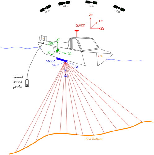
The bathymetric acquisition system consists of, at least, a GNSS (Global Navigation Satellite System) receiver, an IMU (Inertial Measurement Unit) and an acoustic sounder. In this paper, the considered acoustic sounder is the MultiBeam EchoSounder (MBES). The MBES is associated with a sound velocity probe that measures the speed of sound in the water column as well as the sound velocity probe at the sonar head. Each sensor has its own reference frame, the sensors and their respective frames can be observed in Figure 1.

Figure 1. Sensors and frames of a MBES data acquisition system embedded on a vessel.

The data acquired by the different sensors of the acquisition system can be georeferenced using the sounding georeferencing model given in Equation (1)(1) $$X_n\left(t\right)=\mathrm{}{P}_n\left(t\right)+C_I^n\left(t\right)\left(C_S^I\mathrm{}{M}_S\mathrm{}\left(t\right)+\mathrm{}{b}_I\mathrm{}\right)$$(1) . This model is the simplified form of the model proposed by Hare (1995) and used by Debese (Chapter II, 2013), and Seube and Keyetieu (2017). (1) $$X_n\left(t\right)=\mathrm{}{P}_n\left(t\right)+C_I^n\left(t\right)\left(C_S^I\mathrm{}{M}_S\mathrm{}\left(t\right)+\mathrm{}{b}_I\mathrm{}\right)$$(1) where

• $X_n$ is the georeferenced sounding from the measurement acquired by the acquisition system;

• $P_n\left(\mathrm{t}\right)$ is the vector of geographic coordinates ($x_{{\mathrm{P}}_{\mathrm{n}}},\mathrm{}{y}_{{\mathrm{P}}_{\mathrm{n}}},\mathrm{}{z}_{{\mathrm{P}}_{\mathrm{n}}}$) measured by the GNSS receiver in the local navigation frame $n;$

• $C_I^n\left(t\right)$ is the transformation matrix between the local navigation frame $n$ and the IMU frame $I$ using the attitude angles (roll - $\phi ,$ pitch - $\mathrm{Ө},$ heading - $\psi$);

• $C_S^I$ is the transformation matrix between the IMU frame $I$ and the MBES frame $S$ using the boresight angles (${\phi }_b,{Ө}_b,{\psi }_b$);

• $M_S\left(\mathrm{t}\right)$ is the vector related to the sounding coordinates measured in the MBES frame $S;$

• $b_I$ are the lever-arms vector between the IMU and the MBES;

• $t$ is the acquisition time associated to the measurements recorded by the sensors. The time ($t$) is used for the synchronization of the sensors. This time is also considered in the estimation of the latency between the sensors as defined by Bjorn and Einar (2006) and Naankeu Wati, Geldof, and Seube (2016).

The model described in (1) considers the IMU and GNSS receiver are collocated. The COG (Center Of Gravity) is generally established arbitrarily as the reference of the boat frame. The boresight angles (${\phi }_b,$ ${\mathrm{Ө}}_{b\mathrm{}},$${\psi }_b$) used in ${\mathrm{C}}_{\mathrm{S}}^{\mathrm{I}}$ can be determined by the patch test as described by Godin (1998), which implies a predetermined pattern of survey lines. The ${\mathrm{b}}_{\mathrm{I}}$ vector is determined before the survey through the calibration of the acquisition system. This vector contains the distances between the different sensors on the survey vessel.

The $M_S$ vector consists of the sounding coordinates in the $S$ frame calculated from the range ($\rho$) measurements made by the MBES. This distance can be expressed, in a simplified form, by the multiplication of the sound speed in the water column ($s_{\mathit{speed}}$) by half of the travel-time ($\frac{t_{\mathit{\rho }}}{2}$) as mentioned by Lurton (2003). The $s_{\mathit{speed}}$ is measured by the sound velocity probe in the water column. The water column can be modeled by different layers and a refraction occurs when the sound wave goes through a new layer. Hence, the sound wave does not follow a rectilinear trajectory (Beaudoin et al. 2009). Nevertheless, in this paper, for the sake of simplicity, the rectilinear trajectory of the sound wave is adopted and the following expression of $\rho$ is used: ρ = $s_{\mathit{speed}}\frac{t_{\rho }}{2}.$ It is worth mentioning the modelling could be more precise by re-computing the equivalent path assuming a single sound velocity (Hare 1995).

Measurement uncertainties and mathematical model

Several works in the literature addressed the estimation of the uncertainty related to bathymetric data. Hare (1995) documented the mathematical developments of an uncertainty model for bathymetric data acquired by MBES systems (TPU model). In this model, the uncertainty value of each sounded point is estimated using the law of propagation of uncertainty (Joint Committee for Guides in Metrology 2008). This law propagates the uncertainties in the georeferencing model given in (1) considering the bathymetric measurements and its variance-covariance values. The uncertainty model also considers the installation parameters of the sensors in the acquisition system, as the lever-arms and boresight angles estimated by calibration process and its variance-covariance values. The simplified version of the georeferencing model (1) can be rewritten as (2), to lighten the mathematical developments proposed in this section. (2) $${\mathrm{X}}_{\mathrm{n}}\mathrm{}=\mathrm{}{\mathrm{P}}_{\mathrm{n}}\mathrm{}+\mathrm{}{\mathrm{M}}_{\mathrm{n}}+\mathrm{}{\mathrm{b}}_{\mathrm{n}}$$(2) where:

• ${M_n=\mathrm{}C}_I^n\left(t\right){\mathrm{}C}_S^I{M}_S\mathrm{}\left(t\right);$

• $b_n=\mathrm{}{C}_I^n\left(t\right){\mathrm{}b}_I.$

As a result, the estimated uncertainty values ($\mathcal{V})$ of the georeferenced points $X_n$ are given by (3): (3) $${\mathcal{V}X}_n\mathrm{}=\mathrm{}{\mathcal{V}P}_n\mathrm{}+\mathrm{}{\mathcal{V}M}_n+{\mathcal{V}b}_n$$(3)

The uncertainties estimated in (3) are calculated considering:

• the position measurements, namely the GNSS positions ($x_{{\mathrm{P}}_{\mathrm{n}}},\mathrm{}{y}_{{\mathrm{P}}_{\mathrm{n}}},\mathrm{}{z}_{{\mathrm{P}}_{\mathrm{n}}}$) and their uncertainties; they are expressed in the $P_n$ variance-covariance matrix (noted ${\mathcal{V}P}_n$),

• the attitude measurements recorded by the IMU ($\phi ,$ $\mathrm{Ө},$ $\psi$), the boresight angles (${\phi }_b,$ ${\mathrm{Ө}}_{b\mathrm{}},$${\psi }_b$), the sounding distance and pointing angle in the $M_S,$ that are calculated with the travel-time ($t_{\mathit{\rho }}$) and the $s_{\mathit{speed}},$ recorded by the MBES and the sound speed probe and the uncertainties related to these measurements; they are expressed in the $M_n$ variance-covariance matrix (noted ${\mathcal{V}M}_n$),

• the attitude measurements recorded by the IMU ($\phi ,$ $\mathrm{Ө},$ $\psi$), the lever-arms ($a_X,$ $a_{Y\mathrm{}},$$a_Z$) between IMU and MBES and the uncertainties related to these measurements; they are expressed in the ${\mathrm{b}}_{\mathrm{n}}$ covariance matrix (noted ${\mathcal{V}b}_n$),

If latencies are considered in the uncertainty model, the latency between the GNSS receiver and the IMU should be included in ${\mathcal{V}P}_n,$ while the latency between the IMU and the MBES should be included in ${\mathcal{V}M}_n$ and ${\mathcal{V}b}_n.$ In addition, the speed of the platform (${Sp}_X,$ ${Sp}_{Y\mathrm{}},$${Sp}_Z$) should be considered in ${\mathcal{V}P}_n,$ while the angular velocities of the platform (${\omega }_1,$ ${\omega }_{2\mathrm{}},$${\omega }_3$), measured by the IMU, should be considered in ${\mathcal{V}M}_n$ and ${\mathcal{V}b}_n.$ The detailed development of the uncertainty model with the latency considerations can be found in Cassol (2018).

The uncertainties associated to the bathymetric measurements can be either provided by the sensor nominal accuracy, included in the manufacturer technical specifications, or estimated in the data post-processing phase. The bathymetric measurements are recorded by the acquisition system, but their full content may not be easily made available to the hydrographer. Although they are depending on certain information for instance, the format of the acquisition files and the software tools available to read these files. As an example, the hydrographer cannot easily access the IMU recorded values of angular velocities (${\omega }_1,$ ${\omega }_{2\mathrm{}},$${\omega }_3$). Hence, in this case it is not possible to consider the latency value between the IMU and the MBES in the uncertainty estimation. However, this latency shall be considered in the development of the uncertainty model.

Proposed uncertainty value related to the seafloor morphology

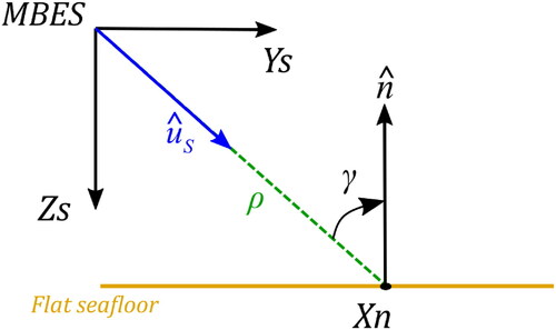
This paper aims to evaluate the influence of the seafloor morphology on the uncertainty of bathymetric data. To evaluate this influence, the uncertainty model given by (3) should also consider the seafloor morphology. This morphological influence on the uncertainty has seldom been investigated in the hydrography field. Hughes Clarke (2018) mentioned that the seafloor detection may vary in the “resulting quality of range estimation as a function of incidence angle”. To this aim, the author proposed to consider a morphological parameter associated with the incidence angle of the georeferenced point. The incidence angle $\mathrm{\gamma }$ is the angle computed between the normal vector (unit vector $\widehat{n}$) of a georeferenced point $X_n$ and the vector supporting the beam $\rho ,$ as shown in Figure 2. A normal can be estimated and associated to each sounded point by considering the plan formed by its neighbors, as shall be further discussed. Please note that the grazing angle of the acoustic beams may also be considered further in this paper. The grazing angle is the complementary angle of the incidence angle. In this Figure, the normal vector of the sounding in the MBES frame ${\widehat{u}}_S$ is also represented. More work has been carried out in the field of airborne LiDAR (Light Detection and Ranging) on a similar topic. The airborne LiDAR is an analogous sensor to the hydrographic system involving a MBES. These works have integrated a contribution of the terrain morphology on the uncertainty value. Studies by Schaer et al. (2007), Goulden (2009) and Goulden and Hopkinson (2010) can be mentioned as examples. Relying on these works, Cassol (2018) proposed a model to assess the morphological uncertainty in LiDAR point clouds recorded with mobile mapping systems. Such a model has been used as the foundation of the model described in this section.

Figure 2. Incidence angle considered in the estimation of the morphological uncertainty.

To consider the morphological component of the error, we propose to decompose the sounding error $\delta \rho$ as the sum of two components ($\delta {\rho }_m$ and $\delta {\rho }_i$). As a result, the measured sounding range ${\rho }_m$ can be expressed as in (4). (4) $${\rho }_m=\rho +\mathrm{}\delta {\rho }_m+\mathrm{}\delta {\rho }_i$$(4) where

• ${\rho }_m$ is the measured distance between the MBES and the seafloor;

• $\rho$ is the measured distance between the MBES and the seafloor without errors;

• $\delta {\rho }_m$ is the measurement error related to the sensors of the bathymetric acquisition system;

• $\delta {\rho }_i$ is the morphological error related to the seafloor morphology.

The measurement error $\delta {\rho }_m$ and its related uncertainty are already included in the ${\mathcal{V}M}_n$ term in the uncertainty model (3). The morphological error $\delta {\rho }_i,$ introduced in this paper, is related to the incidence angle $\gamma$ between the sounding and seafloor. This term is not included in (3). Hence, the sounding error can be expressed as $\delta \rho =\delta {\rho }_m+\mathrm{}\delta {\rho }_i.$ The uncertainty model assumes a flat seafloor, as shown in Figure 2. However, if this assumption is not true, the positioning errors related to the sounded point will occur related to the incidence angle error. Indeed, the normal associated to the sounded point shall differ if the seafloor is flat, sloping or display some morphological pattern. Therefore, the term $\delta {\rho }_i$ can be regarded as the morphological error. Let us denote by ${\mathcal{v}}_{\delta {\rho }_m},$ the uncertainty related to the sounding error $\delta {\rho }_m.$ Similarly, we denote by ${\mathcal{v}}_{\delta {\rho }_i}$ the uncertainty related to the morphological error $\delta {\rho }_i.$

We propose a mathematical model to estimate the influence of the seafloor morphology on the sounded points, also called morphological uncertainty (${\mathcal{v}}_{\delta {\rho }_i}$). This morphological uncertainty shall be further considered in the uncertainty model of the sounded points. To simplify the mathematical demonstrations, the parameters and the measurements considered in (3) will be represented by $\chi \mathrm{}(\phi ,\mathrm{\theta },\psi ,t,{\phi }_b,{\mathrm{\theta }}_b,{\psi }_b,\rho ).$ The error associated to the measurement $\rho$ is $\delta {\rho }_i$ to develop the morphological uncertainty term, since $\delta {\rho }_m$ is already considered in ${\mathcal{V}M}_n$ in (3). Note that the measurements and uncertainties related to the MBES and to the sound speed probe are already considered in ${\mathcal{v}}_{\delta {\rho }_m}$ and should not be considered in the morphological uncertainty (${\mathcal{v}}_{\delta {\rho }_i}$) estimation.

To develop the morphological uncertainty term, we assume that the seafloor neighborhood of the sounded point $X$ can be represented by a plane surface $S(X)=0$ with S a linear equation. This neighborhood is considered to be possible to associate a normal to each sounded point. Since S is a plane, its general expression considering the georeferenced point $X$ is represented in (5) where the coordinates of the georeferenced point X are represented by ($x,\mathrm{}y,\mathrm{}z$). (5) $$S\left(X\right)=\mathrm{}{s}_{1}x+\mathrm{}{s}_{2}y+\mathrm{}{s}_{3}z+\mathrm{}{s}_4$$(5)

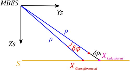
Considering (5), a sounding $X$ belonging to the surface is georeferenced using the parameters $\chi ,$ therefore $S(X(\chi ))=0.$ To estimate the morphological uncertainty, we assume that if we have a small variation $\delta$ in the $\chi$ parameters $\delta \chi ,$ the surveyed point still belongs to S, or in other words $S\left(X(\chi +{\delta }_{\chi })\right)=0.$ Figure 3 illustrates this assumption using an example involving a small variation in roll angle $\delta \phi .$

Figure 3. Represents the position of the sounded point in order to estimate the morphological error. We consider that, even with a small variation in the georeferencing parameters (i.e., roll angle - δφ), the sounding belongs to a plane surface on the seafloor.

Given the plane seafloor assumption for the area near the georeferenced point, the derivative of $S(X(\chi ))=0$ according to $\chi$ can be expressed by (6). (6) $$\frac{d}{d\chi }S\left(X\left(\chi \right)\right)d\chi =0$$(6)

The Equation (6)(6) $$\frac{d}{d\chi }S\left(X\left(\chi \right)\right)d\chi =0$$(6) can be rewritten as (7). (7) $$\frac{d}{dX}S\left(X\right)dX\frac{d}{d\chi }X\left(\chi \right)d\chi =0$$(7)

In (7), $\frac{d}{dX}S\left(X\right)dX$ represents the gradient of $S$ according to $X$ and $\frac{d}{d\chi }X(\chi )$ is the Jacobian matrix of $X$ according to $\chi .$

The partial derivative of S according to the coordinates of $X$ (5) is $\frac{dS}{dX}=\left(s_1,s_2,s_3\right).$ This derivative represents the normal of the local plane. The derivative can also be denoted by $\widehat{n}=\mathrm{}\left(s_1,s_2,s_3\right).$ This normal $\widehat{n}$ relates to the seafloor morphology of the georeferenced point. Accordingly, replacing $\frac{d}{dX}S\left(X\right)dX$ by $\widehat{n},$ (7) becomes (8). (8) $$\widehat{n}\mathrm{}·\mathrm{}\frac{d}{d\chi }X\left(\chi \right)d\chi =0$$(8)

Please note that the $¨·¨$ represents the scalar product in (8). The morphological term of our proposed model is strongly related to the normal vector ($\widehat{n}$) estimated for each sounding. There are different ways to estimate the normal from a group of soundings. In this paper, the normal estimation proposed by Dupont (2020), involving a robust PCA (Principal Component analysis) method, is used. We considered a plan formed by the 10 nearest neighbors to estimate the normal vector ($\widehat{n}$) to associate with each sounded point. This estimation involved all the recorded points acquired on the survey, and not only the points of the swath. Equation (8)(8) $$\widehat{n}\mathrm{}·\mathrm{}\frac{d}{d\chi }X\left(\chi \right)d\chi =0$$(8) can be rewritten using the parameters included in $\chi$ and their partial derivatives. The resulting equation is expressed by (9). (9) $$\widehat{\mathrm{n}}\mathrm{}·\mathrm{}\left(\frac{\partial X}{\partial \phi }\delta \phi +\frac{\partial X}{\partial \mathrm{\theta }}\delta \mathrm{\theta }+\frac{\partial X}{\partial \psi }\delta \psi +\frac{\partial X}{\partial t}\delta t+\frac{\partial X}{\partial {\phi }_b}\delta {\phi }_b+\frac{\partial X}{\partial {\mathrm{Ө}}_{b\mathrm{}}}\delta {\mathrm{Ө}}_{b\mathrm{}}+\frac{\partial X}{\partial {\psi }_b}\delta {\psi }_b+\frac{\partial X}{\partial \rho }\mathrm{\delta }{\mathrm{\rho }}_{\mathrm{i}}\right)=0$$(9)

Based on (9), the morphological error $\mathrm{\delta }{\mathrm{\rho }}_{\mathrm{i}}$ can be estimated considering the parameters ($\phi ,\mathrm{\theta },\psi ,t,{\phi }_b,{\mathrm{\theta }}_b,{\psi }_b$) and the normal $\widehat{n}$ as shown by (10). (10) $$\delta {\rho }_i=\mathrm{}\frac{-\widehat{n}\mathrm{}·\mathrm{}(\frac{\partial X}{\partial \phi }\delta \phi +\frac{\partial X}{\partial \mathrm{\theta }}\delta \mathrm{\theta }+\frac{\partial X}{\partial \psi }\delta \psi +\frac{\partial X}{\partial t}\delta t+\frac{\partial X}{\partial {\phi }_b}\delta {\phi }_b+\frac{\partial X}{\partial {\mathrm{Ө}}_{b\mathrm{}}}\delta {\mathrm{Ө}}_{b\mathrm{}}+\frac{\partial X}{\partial {\psi }_b}\delta {\psi }_b)}{\widehat{n}\mathrm{}·\mathrm{}\frac{\partial X}{\partial \rho }}$$(10)

To simplify the notations in Equation (10)(10) $$\delta {\rho }_i=\mathrm{}\frac{-\widehat{n}\mathrm{}·\mathrm{}(\frac{\partial X}{\partial \phi }\delta \phi +\frac{\partial X}{\partial \mathrm{\theta }}\delta \mathrm{\theta }+\frac{\partial X}{\partial \psi }\delta \psi +\frac{\partial X}{\partial t}\delta t+\frac{\partial X}{\partial {\phi }_b}\delta {\phi }_b+\frac{\partial X}{\partial {\mathrm{Ө}}_{b\mathrm{}}}\delta {\mathrm{Ө}}_{b\mathrm{}}+\frac{\partial X}{\partial {\psi }_b}\delta {\psi }_b)}{\widehat{n}\mathrm{}·\mathrm{}\frac{\partial X}{\partial \rho }}$$(10) , we represent the ratio of the scalar product of the normal vector and partial derivative vector to the scalar product of the normal and partial derivative by the coefficients a_i (for example $a_1=\frac{-\widehat{n}\mathrm{}·\mathrm{}\frac{\partial X}{\partial \phi }}{\widehat{n}\mathrm{}·\mathrm{}\frac{\partial X}{\partial \rho }}$) . With this simplification, the equation can be rewritten as (11). (11) $$\delta {\rho }_i=\mathrm{}{a}_1\delta \phi +a_2\delta \mathrm{\theta }+a_3\delta \psi +a_4\delta t+a_5\delta {\phi }_b+a_6\delta {\mathrm{Ө}}_{b\mathrm{}}+a_7\delta {\psi }_b$$(11)

Using (11) and the uncertainties related to the parameters in $\chi$ (noted ${\mathcal{v}}_{\mathrm{}xx}$ where xx represents one of the $\chi$ parameters) except the sounding range, the uncertainty related to $\delta {\rho }_i$ is given by (12): (12) $${\mathcal{v}}_{\delta {\rho }_i}^2={a_1}^2{{\mathcal{v}}_{\mathrm{}\delta \phi }}^2\mathrm{}+{a_2}^2{{\mathcal{v}}_{\mathrm{}\delta \mathrm{Ө}}}^2+{a_3}^2{{\mathcal{v}}_{\mathrm{}\delta \psi }}^2+{a_4}^2{{\mathcal{v}}_{\mathrm{}\delta t}}^2+{a_5}^2{{\mathcal{v}}_{\mathrm{}\delta {\phi }_b}}^2+{a_6}^2{{\mathcal{v}}_{\mathrm{}\delta {\mathrm{Ө}}_{b\mathrm{}}}}^2+{a_7}^2{{\mathcal{v}}_{\mathrm{}\delta {\psi }_b}}^2$$(12)

Therefore, the georeferencing model (2) can be written as (13) only for the estimation of the morphological uncertainty. In this equation, the term $\delta {\rho }_m$ is considered in $M_n$ term and $\delta {\rho }_i$ is added to estimate the morphological uncertainty. (13) $$X_n\mathrm{}=\mathrm{}{P}_n\mathrm{}+\mathrm{}{M}_n+\mathrm{}{b}_n+\mathrm{}\delta {\rho }_i{C}_I^n\mathrm{}{C}_S^I{\widehat{u}}_S$$(13)

The term $\delta {\rho }_i{C}_I^n\mathrm{}{C}_S^{bI}{\widehat{u}}_S\mathrm{}$ in (13) can be simplified as $S_n.$ The term $S_n$ allows for the observation of the contribution of the morphological uncertainty value to each coordinate of $X_n$ according to ${\widehat{u}}_S.$ Similarly, as the uncertainty values in (3), the morphological uncertainty is computed using the law of propagation of covariance. The covariance matrix of $S_n$ (denoted ${\mathcal{V}S}_n$) associated to the georeferenced point $X_n$ considering the morphological uncertainty ${\mathcal{v}}_{\delta {\rho }_i}^2$ is expressed in (14). (14) $${\mathcal{V}S}_n={\mathcal{v}}_{\delta {\rho }_i}^2{(C}_I^n\mathrm{}{C}_S^I\mathrm{}{\widehat{u}}_S){\left(C_I^n\mathrm{}{C}_S^{bI}\mathrm{}{\widehat{u}}_S\right)}^T$$(14)

The morphological uncertainty of a georeferenced point can be estimated using (14). This estimation uses only the measurements that can have an influence on the morphological uncertainty. With this new morphological uncertainty term now defined, we can update the uncertainty model. It can be expressed as the covariance matrices $P_n,$ $M_n,\mathrm{}{b}_n,$ and $S_n$ as given by (15). (15) $$\mathcal{V}{X}_n\mathrm{}=\mathrm{}{\mathcal{V}P}_n\mathrm{}+\mathrm{}{\mathcal{V}M}_n+{\mathcal{V}b}_n+{\mathcal{V}S}_n$$(15)

This updated uncertainty model will be used to assess the impact of the seafloor on the uncertainty of the georeferenced points. To this end, the values provided by the original uncertainty model (3) will be compared to the values provided by the updated model (15). The relative difference between the uncertainty values will be computed to highlight the significance of the morphology contribution to the uncertainty budget.

Application of the proposed uncertainty model to simulated and real datasets

In this section, we applied the uncertainty model proposed in (15) on simulated and real datasets. The simulated datasets were used to develop the proposed model. Then, we applied the model on a real dataset to better understand the influence of the seafloor morphology on the uncertainty value related to the bathymetric data.

Please note that, in the following, the normal vector of each sounding is considered when estimating the uncertainty related to the seafloor morphology. In addition, the sensor nominal accuracy was used as the uncertainty related to the measurements. This may not be applicable in real hydrographic survey contexts, where such uncertainties may be recorded and made available in survey files.

Simulated datasets

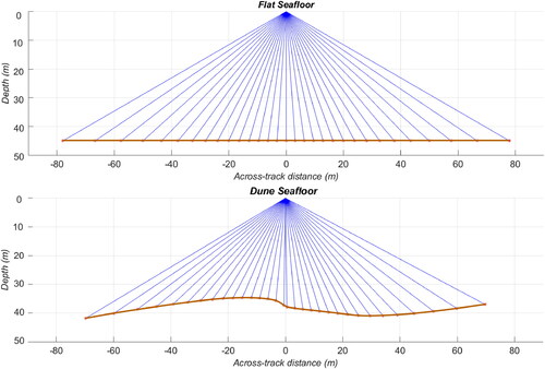
Two simulated datasets were built to apply and validate the uncertainty model proposed in (15). The first one is a flat seafloor and the second one is a seafloor composed by underwater dunes. Profiles related to these two simulated seafloor surfaces are illustrated in Figure 4.

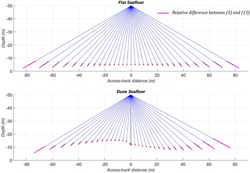
Figure 4. Simulated datasets. The maximum depth is 45 m with a swath angle of 120° represented by soundings every 4° (equiangular acquisition mode). On the top, a simulated flat seafloor profile. On the bottom, a simulated dune profile oriented in the direction of the river current (same direction as Y_S), which is perpendicular to the direction of swath track line.

The sensors considered in the simulation are the same as the ones in the Helen Irene Battle vessel of the CHS (Canadian Hydrographic Service). This acquisition system was used to acquire the real dataset which will be further discussed. The sensors are as follows: the SP90m and PosMV OceanMaster as positioning system and IMU, the Kongsberg EM2040 as MBES, the AML MicroX (AML Oceanographic) as surface speed sensor and the profiler BaseX of AML as sound velocity profiler. The a priori uncertainties and parameters of the sensors are given by the manufacturers and presented in Table 1.

Table 1 . A priori uncertainties and parameters of the acquisition system sensors given by the manufacturers.

Positioning system uncertainties
Measurement	A priori uncertainty
$x_{{\mathrm{P}}_{\mathrm{n}}},$ $y_{{\mathrm{P}}_{\mathrm{n}}}$^a	(5 cm + 1 ppm$\times$ baseline length)
$z_{{\mathrm{P}}_{\mathrm{n}}}$	(8 cm + 1 ppm$\times$ baseline length)
$\phi$ , $\mathrm{Ө}$^b	0.01°
$\psi$^B	0.02°
MBES and sound speed probe uncertainties
Raw range resolution^c	10.5 mm
Maximal angular coverage^c	170°
Sound speed probe^d	0.025 m/s
Sensors installation parameters uncertainties
${\phi }_b,$ ${\mathrm{\theta }}_b,$ ${\psi }_b$^e	0.05°
$a_X,$ $a_{Y\mathrm{}},$$a_Z$^e	1,5 cm

^aSpectra Geospatial (2020).

^bApplanix (2019).

^cKongsberg (2021).

^dAML Oceanographic (2020).

^eConsidered values for the survey involving the survey platform Hele Irene Battle.

To better understand the influence of the seafloor morphology on the uncertainty of the sounded points, we calculated the uncertainty values using the model described in (3). This uncertainty value associated to the georeferenced point shall be considered in this paper as the 3 D combination of the uncertainty related to the coordinates$\mathrm{}x,\mathrm{}y,\mathrm{}z.$ For the flat simulated seafloor, the minimal uncertainty value can be observed at the nadir sounding with a value of 12.6 cm. The values increase up to the outer soundings to a maximal uncertainty value of 17 cm, as it was expected. Considering the dune-simulated seafloor, the minimal uncertainty value of 12.1 cm is also at nadir soundings. The uncertainty values increase up to the outer soundings to a maximal uncertainty value of 16.1 cm. As expected, by using the uncertainty model without taking into account the seafloor morphology (i.e., model described in Equation 3(3) $${\mathcal{V}X}_n\mathrm{}=\mathrm{}{\mathcal{V}P}_n\mathrm{}+\mathrm{}{\mathcal{V}M}_n+{\mathcal{V}b}_n$$(3) ), the same behaviour and uncertainty range of values are observed for the two datasets.

The uncertainties were also estimated considering the seafloor morphology using the proposed model in (15). For the flat seafloor, the minimal uncertainty value is at nadir with a value of 12.7 cm. The uncertainty values increase up to the outer beams to a maximal value of 23.3 cm at the highest grazing beam. The minimum value of uncertainty for the dune seafloor using (15) is 12.2 cm. This value was not estimated for the nadir beam, but for the acoustic beam measuring the crest of the dune (located in the nadir area in Figure 4). Nonetheless, the uncertainty value at nadir is still low with a value of 12.5 cm. The maximal uncertainty can be observed at the outer beams with a value of 26.9 cm.

Comparing the uncertainty values calculated using (3) and (15), we observed no significant difference at the nadir soundings. However, there is a significant difference on the value of uncertainty calculated for the outer beams. For the flat seafloor, this difference is 6.3 cm and for dune seafloor, the difference is 10.8 cm. The difference between the uncertainty estimated with (3) and (15) can be observe on Figure 5.

Figure 5. Relative difference between the uncertainty computed using (3(3) $${\mathcal{V}X}_n\mathrm{}=\mathrm{}{\mathcal{V}P}_n\mathrm{}+\mathrm{}{\mathcal{V}M}_n+{\mathcal{V}b}_n$$(3) ) and (15(15) $$\mathcal{V}{X}_n\mathrm{}=\mathrm{}{\mathcal{V}P}_n\mathrm{}+\mathrm{}{\mathcal{V}M}_n+{\mathcal{V}b}_n+{\mathcal{V}S}_n$$(15) ) representing the influence of the seafloor morphology on the uncertainty value. This difference is due to the ${\mathcal{V}S}_n$ term and can be observed in magenta for each simulated beam sounding (blue lines). The morphological uncertainty estimated by ${\mathcal{V}S}_n$ term has an exaggeration scale of 100 in relation to the soundings distance.

In order to better observe the influence of the seafloor morphology on the uncertainty illustrated on Figure 5, we classified the relative difference between the classical and the proposed model (i.e., $\left[\left(15\right)-(3)\right]/(15)$) according to five classes namely: 0-1%; 1.0 − 5%; 5.0 − 15%; 15.0 − 30%; 30.0 − 100%. The result can be observed on Figure 6.

Figure 6. Relative difference between the uncertainty computed using (3(3) $${\mathcal{V}X}_n\mathrm{}=\mathrm{}{\mathcal{V}P}_n\mathrm{}+\mathrm{}{\mathcal{V}M}_n+{\mathcal{V}b}_n$$(3) ) and (15(15) $$\mathcal{V}{X}_n\mathrm{}=\mathrm{}{\mathcal{V}P}_n\mathrm{}+\mathrm{}{\mathcal{V}M}_n+{\mathcal{V}b}_n+{\mathcal{V}S}_n$$(15) ) representing the influence of the seafloor morphology on the uncertainty value. The relative difference is converted in percentage and presented as a magenta segment attached to the simulated points (blue). The morphological uncertainty estimated by the ${\mathcal{V}S}_n$ term has an exaggeration scale of 100 in relation to the soundings distance.

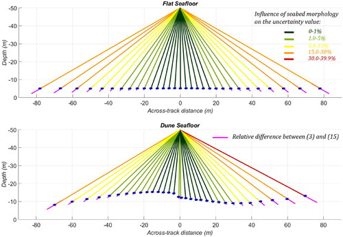
As previously mentioned, and shown in Figure 6, the relative difference is negligible in the flat simulated seafloor with an influence of the seafloor morphology under 1% in the nadir beams. In the outer beams of the swath, this difference is between 15% and 20% and in the outermost beam, approximately 27% of the uncertainty value comes from the morphological uncertainty. For the dune seafloor, the relative difference is still negligible at nadir with a value of approximately 2%. As mentioned earlier, the lowest influence of the seafloor morphology on the uncertainty value is located at the dune crest. Indeed, for this sounding, the uncertainty value is lower than 1%. The influence of the seafloor morphology estimated by the relative difference between (3) and (15) increases up to approximately 40% for the outermost beam (i.e., red beam on Figure 6). This influence is between 15% and 25% in the grazing beams located on the border of the swath (i.e., orange beams on Figure 6). These values shall be further discussed in the fourth section of the paper.

Real dataset

After applying the proposed model considering the seafloor morphology (15) on simulated datasets, the model was tested on a real dataset. This dataset was acquired on the sector G14 of the Northern Traverse of the Saint Lawrence River, near the Orléans Island (Eastern Canada). The sector of this navigation channel includes many underwater sedimentary structures, such as underwater dunes. The survey involved nine lines in the Southwest-Northeast direction. The paper focuses on two selected zones of the G14 sector (i.e., zones A and B), which have relevant morphological characteristics. Nevertheless, the proposed method is scalable to larger areas. The data acquisition system was embedded in the Helen Irene Battle vessel of the CHS. The sensors used in this acquisition are the same as the ones described in the previous section with their a priori uncertainties and parameters described in Table 1. As previously mentioned, the normal vector associated to each sounded point was estimated using a robust PCA method as proposed by Dupont (2020). The DBMs of the zones A and B can be observed in Figure 7. Both DBMs surfaces were computed with processed bathymetric data (e.g., celerity correction, processing of the vessel trajectory) without post-processing filtering.

Figure 7. DBM of zones A and B of the sector G14 of the Northern Traverse of the Saint-Lawrence River. The cell resolution is 1 m. The DBM is computed considering the mean values of the soundings in each cell.

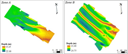
Both surfaces shown in Figure 7 present sedimentary structures (e.g., underwater dunes) on the seafloor surface. Zone A has a minimum depth of 13.45 m and a maximum depth of 22.10 m. In this zone, we can observe the presence of dunes in the eastern side and a relatively flat seafloor in the western side of the zone. Zone B has a similar depth with a minimum of 13.40 m and a maximum depth of 24.75 m. These surfaces shall be used to illustrate the influence of the seafloor morphology on the uncertainty value. Therefore, the uncertainty was estimated for both zones, with the proposed uncertainty model (15). The calculated uncertainty values are presented in Figure 8. This figure also illustrates the survey lines and the crest lines of the dunes aiming to highlight the influence of the seafloor morphology on the uncertainty value. Please note that the computational cost to estimating the influence of the seafloor on the uncertainty from both zones is relatively high (i.e., around twenty hours including the estimation of the normal by the robust PCA method for about 7 million sounded points using a computer with 12 GB RAM and Intel Core i7-3770 @ 3.40 GHz CPU).

Figure 8. Uncertainty values computed with the proposed model including the seafloor morphology, the survey lines (cyan lines) and crest lines of the dunes (magenta). The mean value of the uncertainty was considered at each cell to represent the uncertainty value. The cell resolution is 1 m.

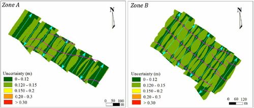
The uncertainty values for both zones are generally inferior to 15 cm with a few isolated soundings with a superior value, but it is not critical on the survey. Similarly, to the simulated datasets, a preliminary estimation of the uncertainty was carried out using the model described in (3) for the dunes real datasets. It can be observed that some areas in the center of zone A have an uncertainty greater than 15 cm. The influence of the morphological parameter on the estimation of the uncertainty is clearly shown in Figure 8. In fact, in the western flat area of zone A, it can also observed that the minimum uncertainty value is located in the near-nadir area of the survey line. The uncertainty is increasing with the grazing angle of the soundings in the swath. In the center of the zone A, we can observe the effect of the seafloor morphology, with the minimum uncertainty on the near-nadir area and in the crest line of the dune. This influence is more significant in zone B, where the uncertainty values have minimum values in the near-nadir area and near the crest line of the dunes. The classified relative difference for the real dataset can be observed in Figure 9. Please note that different classes were used to highlight the relative difference between (3) and (15), namely: 0-1%; 1.0 − 5%; 5.0 − 10%; 10.0 − 15%; 15.0 − 100%.

Figure 9. The influence of the seafloor morphology on the uncertainty considering the underwater dune context, the survey lines (cyan lines) and crest lines of the dunes (magenta). The mean value of the relative uncertainty was considered at each cell. The cell resolution is 1 m.

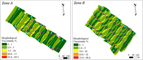
The morphological influence on the uncertainty value is more spatially variable in the underwater dune context. We can compare the flatter areas of zone A (eastern and western areas) with the dune seafloor. For flat seafloor areas, close to the nadir, the majority of the surface cells had a contribution lower than 1%. This value of relative difference increases with the grazing angle in the outer beams of the swath. In the dune areas, specifically, in zone A, the relative uncertainty is ranging between 5% and 15% in the outer beams of the swath over the dunes. The relative difference of some cells of the DBM is superior to 15% being related to noisy points considered in our analysis. Noisy points often yield errors in the normal estimation, which is associated to the sounded points considered in the proposed model. In zone B, the influence of the morphological parameter is more significant. A higher spatial variability of the uncertainty values is observed. The influence of the morphological parameter is lower than 1% in the near nadir area and near the crest lines of the dunes. This is due to the fact that the crest lines are closer to the survey platform and do not present acute grazing-angle beams. The relative uncertainty increases up to 15% in the outer beams of the swath, especially in the valley zone between the dunes, where the sounding beams present an acute incidence angle. Thus, this is where the morphological parameter has the stronger impact.

Discussion

This section aims to further discuss the results presented in the previous section and the strength and limitations of the proposed complementary model. The influence of the seafloor on the uncertainty value, estimated by the relative difference between (3) and (15), was negligible in the beams at nadir of the simulated and the real datasets. In both datasets, this influence increases on the outer beams of the swath. This growth is related to the grazing angle between the beam and the seafloor surface. Since this influence is directly associated to the seafloor morphology, higher values could be located anywhere on the swath, not necessarily on the outer beams. The relationship between the seafloor morphology (i.e., normal associated to the sounded point) and the morphological uncertainty proposed in this paper can be observed in Figure 10, where the difference between the sounding range uncertainties ${\mathcal{v}}_{\delta {\rho }_m}$ and ${\mathcal{v}}_{\delta {\rho }_i}$ considered in (15) are presented.

Figure 10. The uncertainties related to the sounding errors (${\mathcal{v}}_{\delta {\rho }_m}\text{and}{\mathcal{v}}_{\delta {\rho }_i}$) can be observed in different seafloor contexts.

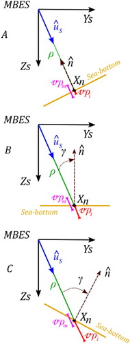
In the first geometry example (Figure 10.A), the incidence angle is equal to zero (where $\widehat{n}=\mathrm{}-{\widehat{u}}_S$). Therefore, the morphological uncertainty (${\mathcal{v}}_{\delta {\rho }_i}$) has also a near-zero value since the morphological error is strongly related to the incidence angle $\mathrm{\gamma }.$ In a flat seafloor context (Figure 10.B), the value of ${\mathcal{v}}_{\delta {\rho }_i}$ is greater than in Figure 10.A since the incidence angle is greater to 0. In Figure 10.C, the uncertainty related to the seafloor morphology increases when comparing with Figure 10.A and Figure 10.B. Indeed, such increase is directly related to the increase of the incidence angle. The morphological uncertainty has its maximum values in the grazing angle areas where (${\widehat{u}}_S\perp \mathrm{}\widehat{n}$). Regarding the value of ${\mathcal{v}}_{\delta {\rho }_m},$ it remains the same in the three examples since it considers the bathymetric measurements and its related uncertainty. Therefore, the uncertainty value associated to the soundings increases with the grazing angle which is consistent with Tidd (2005) observations. Furthermore, the study states that the swath of the MBES is limited by the grazing angles. Therefore, “a seafloor which results in acute incident angles throughout the swath can be reasonably expected to provide reduced quality data” (Tidd 2005).

The influence of the seafloor morphology on the uncertainty located in the near nadir area for the simulated and real datasets are consistent with each other. Nonetheless, the range of the influence calculated for the outer beams of the simulated datasets are not in the same order as the one for the real datasets, especially the outmost beam value (i.e., 27% for flat seafloor and 40% for dune seafloor). These values can be directly associated to the grazing angle between these acoustic beams and the seafloor surface, as illustrated in Figure 10.C. In these simulated datasets, the outermost beams are characterized by more acute grazing angles, which may be avoided in a real data acquisition.

As synthetized in Figure 10, the model proposed in (15) is intimately related to the estimation of the normal associate to each sounded point. The estimated normal can be affected by the noise that can be present in the bathymetric data. Even if the normal computation with the robust PCA limit the noise influence, caution must be taken when interpreting the influence of seafloor morphology on the estimated uncertainty considering the proposed model (15). There would then be a combination of the morphology influence on the uncertainty value with the noise effect. In areas affected by noisy data, the influence of the seafloor morphology on the uncertainty exceeds 15%. However, in the real dataset shown in Figure 9, the noise is limited to outer beams of the swath being even difficult to observe in this figure. Furthermore, the anticipated use of the proposed model (15) concerns the post-processing phase. As a result, at that stage, most of the noisy points should be already filtered. Further experiments considering the proposed model (15) may also estimate the normal associated to each sounding from the DBM. Such estimation should evaluate not only the sensitivity related to the estimation of the normal from the bathymetric point cloud or from the DBM, but also the computational speed advantage related to the normal estimation.

As argued above, the anticipated use of the proposed model (15) should be in the post-processing phase, specifically in the data analysis stage. This information can be very helpful in the study of the sedimentary structures present on the seafloor surface (e.g., Debese, Jacq, and Garlan 2016; Di Stefano and Mayer 2018). The characterization of these structures generally involves locating their salient features. For example, in the case of underwater dunes, we would try to locate the crest line. At that stage, the uncertainty estimated with (3) is available. It essentially characterizes the uncertainty related to the acquisition system. What the proposed model brings here is the ability to improve the interpretation of the uncertainty according to the position of the sounding on the dune. As such, not only would the crest line be characterized, but also the uncertainty variation along the crest line would be available. This complementary information could be useful when studying the spatiotemporal variation of the detected structures and saliences. The knowledge of the morphological uncertainty could help discriminate real migration from location discrepancy related to the data uncertainty.

Conclusion

An estimation of the influence of seafloor morphology on the bathymetric data has been proposed in this paper. It relies on the classical georeferencing model, the bathymetric survey measurements, and their related uncertainties. The proposed model adds a new term, called the morphological uncertainty, to the classical uncertainty estimation model. It represents the contribution of the seafloor morphology to the uncertainty value. This representation relies on the incidence angle of the acoustic beams.

In addition to the proposed model, the second contribution of this work is the analysis of the influence of the seafloor morphology on the uncertainty of the bathymetric data. The relative differences between the uncertainties estimated by the classical model (3) and the proposed model (15) highlighted the impact of the morphological parameter. This difference was computed for simulated datasets, which were used to validate the model, and a real dataset. The latter, acquired by the Helen Irene Battle vessel of the CHS over a dune seafloor, shows an influence of the seafloor morphology on the uncertainty value up to 15% in almost all of the surfaces, with a few noisy points, presenting an influence greater than 15%. Such a contribution was mostly due to the incidence angle of the beam which varies significantly given the changing seafloor morphology induced by the dunes. The uncertainty increases with the grazing angle beams, such grazing being associated with beams in the swath outer part or with the presence of a particular bottom morphology located anywhere on the swath. Finally, the paper addressed the normal computation in the proposed model, which makes its involvement necessary in the post-processing phase. However, if this model is applied to noisy data, some care would be required when interpreting the uncertainty results, since the noise and morphological effect may be combined.

Acknowledgments

The authors would like to thank Université Laval for providing access to the equipment and laboratories required to conduct this research. Also, the authors thank the CIDCO (Centre Interdisciplinaire en Développement en Cartographie des Océans), Mathieu Rondeau and Ghislain Bouillon of the Canadian Hydrographic Service (CHS) for providing the data used in this research. Thanks to the companies for the licenses of the software as QPS for Qimera 1.7.6, ESRI for ArcGIS 10.7 and Matlab R2019a—Classroom use. The authors acknowledge Vincent Dupont, M.Sc., for his comments and involvement in the results production phase.

Disclosure statement

The authors declare no conflicts of interest.

Data availability statement

The data are not publicly available. The data were a courtesy of the Canadian Hydrographic Service for this research. They can be available upon request to the corresponding author.

Additional information

Funding

This work was supported by the FRQ-NT (Fonds de Recherche Nature et Technologie Québec) under grant 2018-PR-206875. The authors thank Mitacs, CN (Canadien National), Faculté de Foresterie, Géographie et Géomatique de l’Université Laval, Fond Joncas, l’Association de Géomatique Municipale du Québec (AGMQ) and Canadian Institute of Geomatics (CIG) for their financial support.

References

- Amante, C. J., and B. W. Eakins. 2016. Accuracy of interpolated bathymetry in digital elevation models. Journal of Coastal Research 76:123–33.
- AML Oceanographic. 2020. Base-X product description. Accessed December 7, 2021. http://www.mdsys.co.kr/down/AML/Base_X.pdf.
- AML Oceanographic. Micro-X product description. Accessed December 7, 2021. https://stema-systems.nl/wp-content/uploads/2015/08/Micro-X_Brochure.pdf.
- Applanix. 2019. POS MV OceanMaster, 2. Accessed December 7, 2021. https://www.applanix.com/downloads/products/specs/posmv/POS-MV-OceanMaster.pdf.
- Beaudoin, J., B. Calder, J. Hiebert, and G. Imahori. 2009. Estimation of sounding uncertainty from measurements of water mass variability. International Hydrographic Review November 2009:20–38.
- Bjorn, J, and B. Einar. 2006. Time referencing in offshore survey systems. FFI/RAPPORT-2006/01666. Forsv Arets Forskninginstitutt (Norwegian Defence Research Establishment), 122.
- Byrne, J. S, and V. E. Schmidt. 2015. Uncertainty modeling for AUV acquired bathymetry. U. S. Hydrographic Conference (US HYDRO), Gaylord Hotel, National Harbor, Maryland, USA, 25
- Calder, B. R., and L. A. Mayer. 2003. Automatic processing of high-rate, high-density multibeam echosounder data. Geochemistry Geophysics Geosystems 4 (6):22.
- Canadian Hydrographic Service (CHS). 2012. Traitement et analyse de données bathymétriques de CUBE. Pêches et Océans Canada, 7 p.
- Cassol, W. N. 2018. Définition d'un modèle d'incertitude-type composée pour les Systèmes LiDAR mobiles, Master thesis, Université Laval, Québec, Canada, 111 p.
- Debese, N. 2013. Bathymétrie. Sondeurs, traitements des données, modèles numériques de terrain. Cours et exercices corrigés. Paris, France: TECHNOSUP, éditions ellipses, 404 p.
- Debese, N., J. J. Jacq, and T. Garlan. 2016. Extraction of sandy bedforms features through geodesic morphometry. Geomorphology 268:82–97.
- Di Stefano, M., and L. A. Mayer. 2018. An automatic procedure for the quantitative characterization of submarine bedforms. Geosciences 8 (1):28.
- van Dijk, T. J. A. van Dalfsen, V. Van Lancker, R. A. van Overmeeren, S. van Heteren, and P. J. Doornenbal. 2012. 13—Benthic habitat variations over tidal ridges, North Sea, the Netherlands. In Seafloor Geomorphology as Benthic Habitat; 241–9. Elsevier: Amsterdam, The Netherlands. ISBN 9780123851406.
- Dupont, V. 2020. Élaboration d’une méthode d’extraction de plans par croissance de régions dans un nuage de points bathymétriques servant à alimenter des estimateurs d’erreur hydrographique. Université Laval, Québec, Canada, 120 p.
- Godin, A. 1998. The calibration of shallow water multibeam echo-sounding systems. Fredericton, Canada: Department of Geodesy and Geomatics Engineering, University of New Brunswick, 76–120.
- Goulden, T. 2009. Prediction of error due to terrain slope in LiDAR observations. Technical Repport no. 265. Department of Geodesy and Geomatics Engineering, University of New Brunswick, 150 p.
- Goulden, T., and C. Hopkinson. 2010. The forward propagation of integrated system component error within airborne LiDAR data. Photogrammetric Engineering & Remote Sensing 76 (5):589–601.
- Hare, R. 1995. Depth and position error budgets for multibeam sounding. International Hydrographic Review, Monaco LXXII (2):37–69.
- Hare, R., B. Eakins, and C. Amante. 2011. Modelling bathymetric uncertainty. International Hydrographic Review November 2011: 31–42.
- Hughes Clarke, J. E. 2018. The impact of acoustic imaging geometry on the fidelity of seabed bathymetric models. Geosciences 8 (4):109.
- International Hydrographic Organization. 2020. Standards for Hydrographic Surveys, No. 44, 6th ed., 49 p. Principauté de Monaco: IHO Publication.
- Joint Committee for Guides in Metrology. 2008. Evaluation of measurement data—Guide to the expression of uncertainty in measurement. 1st ed., September 2008, 134 p. Sèvres, France: Bureau International des Poids et Mesures (BIPM).
- Kongsberg. 2021. EM 2040 multibeam Echosounder, 2 p. Accessed December 7, 2021. https://www.kongsberg.com/contentassets/e8fa4f09f25f4b1e86eda52cc1355dc7/em-2040–-mkii-data-sheet.pdf
- Lecours, V., M. F. J. Dolan, A. Micallef, and V. L. Lucieer. 2016. A review of marine geomorphometry, the quantitative study of the seafloor. Hydrology and Earth System Sciences 20 (8):3207–44.
- Lurton, X. 2003. Theoretical modelling of acoustical measurement accuracy for swath bathymetric sonars. International Hydrographic Review 4 (2):17–30.
- Naankeu Wati, G., J. B. Geldof, and N. Seube. 2016. Error budget analysis for surface and underwater survey system. International Hydrographic Review May 2016: 21–46.
- Schaer, P., Skaloud, J., Landtwing, S. and Legat, K. 2007. Accuracy estimation for laser point cloud including scanning geometry. 5th International symposium on mobile mapping technology, Padova, Italy, May 29–31, 8 p.
- Seube, N., and R. Keyetieu. 2017. Multibeam echo sounders-IMU automatic boresight calibration on natural surfaces. Marine Geodesy 40 (2–3):172–86.
- Spectra Geospatial. 2020. SP90m GNSS receiver, 3 pages, viewed June 2021.
- Thibaud, R., G. Del Mondo, T. Garlan, A. Mascret, and C. Carpentier. 2013. A spatio-temporal graph model for marine dune dynamics analysis and representation. Trans GIS 17:742–62.
- Tidd, R. A. 2005. The impact of varying seafloor topographies, and object geometris on resolution for multibeam echosounders and multi-angle swath bathymetry systems. Proceedings of OCEANS 2005 MTS/IEEE, Washington DC,Vol. 3,2224–2227.