Lead Detection in the Arctic Ocean from Sentinel-3 Satellite Data: A Comprehensive Assessment of Thresholding and Machine Learning Classification Methods

Abstract

In the Arctic Ocean, obtaining water levels from satellite altimetry is hampered by the presence of sea ice. Hence, water level retrieval requires accurate detection of fractures in the sea ice (leads). This paper describes a thorough assessment of various surface type classification methods, including a thresholding method, nine supervised-, and two unsupervised machine learning methods, applied to Sentinel-3 Synthetic Aperture Radar Altimeter data. For the first time, the simultaneously sensed images from the Ocean and Land Color Instrument, onboard Sentinel-3, were used for training and validation of the classifiers. This product allows to identify leads that are at least 300 meters wide. Applied to data from winter months, the supervised Adaptive Boosting, Artificial Neural Network, Naïve-Bayes, and Linear Discriminant classifiers showed robust results with overall accuracies of up to 92%. The unsupervised Kmedoids classifier produced excellent results with accuracies up to 92.74% and is an attractive classifier when ground truth data is limited. All classifiers perform poorly on summer data, rendering surface classifications that are solely based on altimetry data from summer months unsuitable. Finally, the Adaptive Boosting, Artificial Neural Network, and Bootstrap Aggregation classifiers obtain the highest accuracies when the altimetry observations include measurements from the open ocean.

Keywords:

• Arctic Ocean
• classification
• lead detection
• machine learning
• Sentinel-3
• synthetic aperture radar

Introduction

The Arctic Ocean is highly affected by global warming. The region is subject to temperature changes of about three times the global average (IPCC 2021), of which the Arctic sea ice decline is a major consequence. In only two decades, the perennial sea ice cover has decreased by 50%, and the remainder will likely be lost by 2050 (Kwok 2018). Since changes in the Arctic Ocean have a global impact, the region is of great scientific interest. However, due to the remote location of the Arctic and its relatively harsh environmental conditions, the availability of observational input is limited. For instance, information on the Arctic Ocean sea surface height (SSH) is needed for many purposes; from studying the influence of Arctic glacier melt on the regional sea level (e.g., Cazenave et al. 2019; Rose et al. 2019) to monitoring sea ice thickness (e.g., Laxon et al. 2013; Wernecke and Kaleschke 2015). Unfortunately, in situ data are limited to a few tide gauges at the coast and the presence of sea ice hampers measurements by satellite altimeters. In this respect, Synthetic Aperture Radar (SAR) altimetry provides a solution. SAR altimeters have a higher along-track resolution compared to conventional radar altimeters (Donlon et al. 2012), which allows measuring the SSH through fractures in the sea ice, so-called leads. However, this requires careful discrimination between measurements from sea ice and leads.

Fortunately, because of differences in the surface characteristics of sea ice and leads, these surfaces typically cause distinct SAR returns. Consequently, various classification methods have been developed that use waveform features, which describe the unique features of the SAR return signal. Empirical methods, reliant on setting thresholds for these waveform features, have been widely used to classify radar returns (e.g., Laxon 1994; Peacock and Laxon 2004; Poisson et al. 2018; Zakharova et al. 2015). More recently, machine learning-based classification methods have gained popularity (e.g., Dettmering et al. 2018; Lee et al. 2016; Müller et al. 2017; Poisson et al. 2018). Machine learning-based methods can produce higher accuracies as they can overcome shortcomings associated with the simple thresholding methods, such as failing to deal with waveform features that contain aliasing between leads and sea ice (Lee et al. 2016).

Despite the promising implementations of machine learning classifiers presented in earlier studies, some uncertainties remain. Firstly, the aforementioned classifiers and their performances cannot be directly compared as these studies involve different study areas, sensors, and validation data. For instance, it is still unknown whether unsupervised machine learning classifiers can outperform supervised learning classifiers. Secondly, the validation in previous studies was often limited, e.g., to small areas (Dettmering et al. 2018: the Greenland Sea for unsupervised classification) or few SAR data (Lee et al. 2016: 239 waveforms). The most important restriction on the extent of validation is the need to generate ground truth data, which is often done through visual inspection (Lee et al. 2016, Quartly et al. 2019). As a result, it remains unknown whether the classifier performance is location-dependent. This may, for instance, be due to regional variations in the prevailing sea ice type (e.g., first-year ice or multi-year ice). Thirdly, seasonal differences in classification performance are poorly understood, as lead detection methods are typically only tested on data from winter months. Shu et al. (2020) tested their classifier on data from spring (up to May) and showed reduced performance for May compared to earlier months. In contrast, Dawson et al. (2022) recently obtained comparable performances for the classification of data from winter and summer months.

The main objective of this paper is to provide a comprehensive assessment of lead detection methods, applied to SAR altimetry. Therefore, supervised- and unsupervised machine learning methods and a thresholding method are applied to a wide range of study areas in the Arctic Ocean, to identify the most suited classifier to be applied for SSH estimation. A key opportunity is recognized in using data from the Sentinel-3 satellites (operated by ESA and EUMETSAT), as these satellites are equipped with a Synthetic Aperture Radar Altimeter (SRAL) and the Ocean and Land Color Instrument (OLCI). Therefore, classification methods applied to data acquired by SRAL can be validated using simultaneously acquired OLCI images. This combination of temporally aligned data sources is extremely beneficial to the research as it eliminates the need to employ ice drift models to correct for the relocation of the ice in-between the measurements (Quartly et al. 2019). Although an operator-controlled selection of cloud-free images is required, most of the validation data generation process is successfully automated. In this way, a larger study area can be included in the validation. The classifiers are additionally applied to data from different years and summer months to gain insight into temporal effects. Finally, as part of the Arctic Ocean is completely ice-free during summer months, the classifiers are also tested with consideration of data from the open ocean.

In the following sections, we first expand on the Sentinel-3 satellite data that were used, the procedures that were adopted for generating the ground truth data, the specific classifiers that were implemented, and the measures that were used to assess the classifier performance. Thereafter, the different test cases are introduced, followed by the results and a discussion of the main findings. A list of all abbreviations used in the paper is incorporated in Appendix 5. List of Abbreviations.

Data

Synthetic Aperture Radar Altimeter (SRAL)

This study uses SAR altimetry level 1B data (non-time critical), retrieved by the Synthetic Aperture Radar Altimeter (SRAL) instrument of the Sentinel-3A and Sentinel-3B satellites (Donlon et al. 2012). In contrast to conventional altimeters, SAR altimeters obtain a relatively high along-track resolution by applying coherent processing of groups of transmitted pulses, exploiting the Delay-Doppler effect (Raney 1998). The along-track resolution is ∼300 m (Donlon et al. 2012). The shape of the returned signal relates to the roughness and orientation of the surface from which the signal is reflected. For instance, smooth surfaces such as leads cause specular returns, while rougher surfaces like sea ice and open ocean result in diffuse reflections (Laxon et al. 2013; Poisson et al. 2018). In this paper, the full waveforms (128 data points) were reduced to twelve waveform features (see Figure 1 and Table 1), which were then used as input for the classifiers.

Figure 1. An example of Sentinel-3 SRAL level 1B waveform return from sea ice. The waveform features maximum power (MAX), leading edge width (LeW), trailing-edge width (TeW), and the waveform width (ww) are presented in the figure.

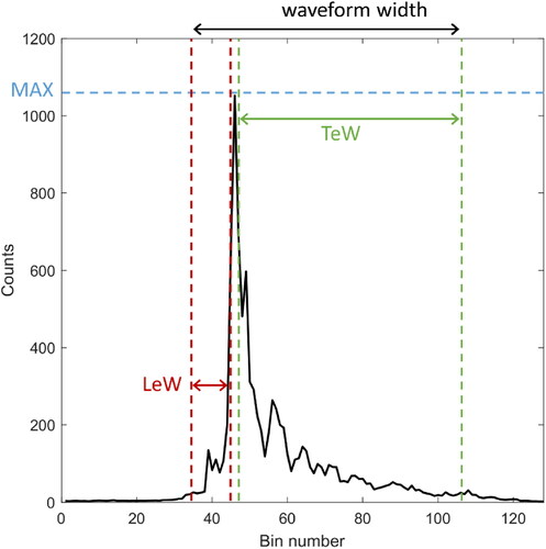
Table 1. Description and equation of the waveform features considered in this study. Here n is the number of bins that make up the waveform, P the power of an individual bin, the P average power, P_max the maximum power, and the standard deviation of the distribution.

Waveform parameter (Abbreviation)	Description	Equation
Maximum Power (MAX)	The maximum power value of the waveform in counts	–
Kurtosis (kurt)	A measure of peakiness of the power distribution (Lee et al. 2016). Kurtosis is a fourth standardized moment.	$\mathrm{kurt}=\frac{1}{n}\mathrm{}\frac{{\sum }_{i=1}^n{\left(P_i-\overline{P}\right)}^4}{{\sigma }^4}$
Skewness (skew)	A measure of how slanted the power distribution is. Skewness is a third standardized moment.	$\mathrm{skew}=\frac{1}{n}\mathrm{}\frac{{\sum }_{i=1}^n{\left(P_i-\overline{P}\right)}^3}{{\sigma }^3}$
Pulse Peakiness (PP)	A measure of the peakiness of the waveform. It is found by dividing the maximum power by the total accumulated power of the waveform (Wernecke and Kaleschke 2015).	$\mathrm{PP}=\frac{P_{\mathit{max}}}{{\sum }_{i=1}^n{P}_i}$
Waveform width (ww)	The number of bins surrounding the peak with a power of at least 1% of the maximum power (Dettmering et al. 2018) (see Figure 1).	–
Leading edge Width (LeW)	The number of bins before the peak that has 1% to 99% of the maximum power value (see Figure 2.1).	–
Trailing edge Width (TeW)	The number of bins after the peak that has 99% to 1% of the maximum power value (see Figure 2.1).	–
Backscatter Coefficient (sigma0)	The radar backscatter coefficient describes the surface properties, radar frequency, polarization, and incident angle (Wingham et al. 2006). Sigma0 values are computed as in CLS (2011), using the maximum power from the original waveform.	–
Pulse Peakiness Left (PPL)	Modified PP, only considering the three bins on the left of the bin belonging to the maximum (Ricker et al. 2014).	$\mathrm{PPL}=\frac{P_{max}}{\sum _{i=i_{max}-3}^{i_{max}-1}{P}_i}$
Pulse Peakiness Right (PPR)	Modified PP, only considering the three bins on the right side of the bin belonging to the maximum (Ricker et al. 2014).	$\mathrm{PPR}=\frac{P_{max}}{\sum _{i=i_{max}+1}^{i_{max}+3}{P}_i}$
Pulse Peakiness local (PPloc)	Modified PP, only considering the three bins on the left and three bins on the right of the bin with maximum power.	$\mathrm{PPloc}=\frac{P_{max}}{\sum _{i=i_{max}-3}^{i_{max}+3}{P}_i}$
Number of Peaks (NrPeaks)	Number of peaks with a peak prominence greater than 5% and a minimum separation distance of five bins	–

Ocean and Land Color Instrument (OLCI)

Optical images taken by the Ocean and Land Color Instrument (OLCI) onboard the Sentinel-3 satellites were used to create ground truth data for the training and validation of the SAR altimetry-based classification. OLCI is a push-broom imaging spectrometer that contains 21 spectral bands (Oa1–Oa21) ranging from 400 nm to 1020 nm (Donlon et al. 2012). This study used the level 1B product, which consists of top of atmosphere radiances, calibrated to geophysical units (Wm⁻²sr⁻¹mm⁻¹), georeferenced onto the Earth’s surface, and spatially resampled onto an evenly spaced grid (Donlon et al. 2012). Pseudo-color images were constructed using three spectral bands from the OLCI data, which are; Oa3 (442.5 nm), Oa5 (510 nm), and Oa8 (665 nm). In these images, water surfaces (leads/open ocean) can be identified as darker areas (lower radiance value) compared to the brighter ice sheets. The images have a spatial resolution of 300 × 300 m (Donlon et al. 2012), which thus limits lead detection to leads that are at least 300 m wide. Nevertheless, the use of these images provides a common ground to compare different classification schemes.

Study areas and dates

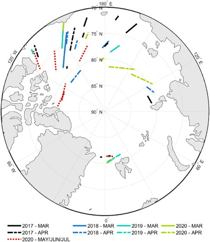
The selection of SRAL tracks was based on the different experiments (see section Experimental Set-up) and the availability of cloud-free OLCI images (manually selected). In total, 35 OLCI images and 18,242 SAR waveforms were collected (see Figure 2). The polar nights and reduced lighting conditions experienced in most winter months restricted the use of OLCI data to images from March, April, and summer months. For the experiments with the extra open ocean class, an additional track was used that crosses the Atlantic Ocean from 50^oS to 50^oN (sensed on August 19, 2021). It was assured that the ocean dataset covers various significant wave heights (SWH; Timmermans et al. 2020) as the SWH determines the curvature of the leading edge of the SAR waveforms and thereby directly affects some of the waveform features (Fenoglio-Marc et al. 2015). Moreover, it was checked that the data were not corrupted by sea ice or land reflections and therefore, no optical data was required for creating the ground truth data. In total, 10,862 open ocean waveforms were included.

Figure 2. The Sentinel-3A/3B SRAL tracks from March 2017 to July 2020 that are used in this paper. Source: Authors.

Methods

Generation of ground truth data

Before testing the classifiers, the SRAL data needed to be labeled according to the ground truth. This procedure relied on a two-step processing of the OLCI product. Firstly, the pseudo-color images were converted to binary images, where each pixel was defined as either lead or sea ice. The following procedure was adopted, inspired by Hamada, Kanat, and Adejor (2019):

1. The study areas were cropped to smaller sections surrounding the SRAL tracks spanning about 0.6° longitude. This was mainly done to reduce the impact of clouds in unused sections of the images on the image segmentation and instead focus on local along-track radiation differences.

2. The images were segmented using Kmeans clustering, considering two clusters (K = 2). This algorithm assigns each pixel to the nearest cluster using the radiance values, while minimizing the total distance to the mean of the clusters. This resulted in binary images.

3. Each point of the SRAL track was assigned a class based on the majority vote of the three closest pixels on the binary images. Three pixels were used to determine the class label because the SRAL data may reflect the surface properties of a combination of pixels, especially when the SRAL data point is located on the edge of a pixel. SRAL data points at the edges of the cropped images were omitted.

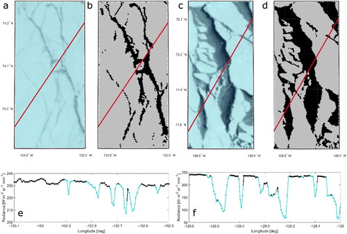
Because this approach to image segmentation relies only on local radiance differences, this method allows for an efficient and flexible application to different study areas. It is not necessary to adjust the approach to correct for e.g., differences in lighting conditions. In Figure 3, two examples of a segmented binary image (b, d) are shown next to their original images (a, c). In some instances, small-scale irregularities in radiance intensity (e.g., due to the presence of small clouds) caused the image segmentation to incorrectly label some pixels. Therefore, a second step was implemented that labels pixels based on relative along-track changes in radiance, as follows:

Figure 3. Examples of OLCI images (a, c) and their binary images after the image segmentation scheme (b, d). The red line shows the Sentinel-3 ground track. The optical images were taken on 15/04/2018 (a) and 13/04/2019 (c). For both examples, the radiance along the ground track for OLCI band Oa3 is shown below (e, f). The colored parts of the line indicate possible leads.

1. The OLCI radiances were interpolated to each SRAL data point.

2. Maximum and minimum peaks in the radiance series were identified as data samples that are, respectively, higher or lower than both neighboring samples.

3. Minimum peaks whose value does not exceed 2% (empirically determined) of the value of the preceding maximum peak were considered to be leads (see Figure 3e, f).

This second step helped to properly label points close to the edge of the leads. SRAL data were only labeled as leads in the ground truth data when this followed from both steps of the procedure. This resulted in a total of 11,762 sea ice and 2,961 lead data points. 3,519 waveforms were rejected.

Classifier configuration and performance assessment

A total of twelve classifiers were assessed in this study, including nine supervised machine learning classifiers, two unsupervised machine learning classifiers, and one thresholding classifier (listed in section Waveform Classifiers).

Waveform classifiers

The following classifiers were implemented in MATLAB®, using functions from the Statistics and Machine Learning toolbox and the Classification Learner application.

Supervised machine learning classifiers

Supervised machine learning classifiers infer a model from labeled training data, consisting of waveform features (cohesively referred to as the feature space) and the corresponding classes. Subsequently, the model is used to predict the classes of a new set of waveform features. The following nine supervised learning classifiers were tested in this study:

• Decision tree-based classification: various tree-based models have been applied to the classification problems and have shown promising results in many remote sensing applications (Shu et al. 2020; Xu, Li, and Brenning 2014), including lead detection (Lee et al. 2016). One can distinguish between single decision tree classifiers and tree-based ensemble classifiers that combine many classification trees for better and more robust predictions (Hastie, Tibshirani, and Friedman 2009). Ensemble tree classifiers are built with many decision trees in parallel (bagging) or sequence (boosting). For this paper, we implemented four types of tree-based classifiers with varying model complexities:

• • • A decision tree (DT) consists of a recursive partition of the input data in a single tree-like structure. At each split, a decision is made based on the input features and the new branches represent the possible outcomes, ultimately leading to the final class labels. DT algorithms develop conditions at each split such that the error of class labels is minimized and a meaningful relationship between a class and the values of its features can be captured (Quinlan 1986). The tuning parameters of this classifier include the maximum number of splits and the type of split criterion that is used to evaluate the effectiveness of a split (Tangirala 2020).

  • • Bootstrap Aggregation (Bagged) relies on building many decision trees based on random subsets of the training data (bootstrapping). The final classification is then determined using the average of all predictions from different trees. This reduces the sensitivity to the training data, and reduces variance and over-fitting compared to DT and boosting ensembles (Breiman 1996). The tuning parameters include the maximum number of splits, number of trees, and learning rate.

  • • Adaptive Boosting (AdaBoost) is an ensemble classifier that attempts to improve the model by iteratively combining DTs (Freund and Schapire 1999). With each iteration, AdaBoost assigns higher weights to misclassifications. In contrast to the Bagged classifier, the boosting method increases the complexity of the model to primarily reduce the bias and reduce any under-fitting of the training data (Breiman 1996). The tuning parameters include the maximum number of splits and the number of trees.

  • • RUSBoost is another boosting method that applies random undersampling (RUS) of the data. Samples from the larger class are randomly removed to ensure a given ratio between the amount of data per class. This improves classification performance, especially for data sets with uneven class sizes (Seiffert et al. 2008). This method can be promising due to the smaller number of leads compared to sea ice data points in the dataset. Tuning parameters include the maximum number of splits, number of trees, learning rate, and class ratio.

• Artificial Neural Network (ANN): ANN is one of the most popular machine learning methods and has been earlier applied to waveform classification (e.g. Poisson et al. 2018; Shen et al. 2017). In this paper, a simple feedforward network was used that consists of an input layer (observations), a few hidden layers, and an output layer (assigned classes). Each layer consists of several so-called neurons that are connected with neurons from adjacent layers (Grossi and Massimo 2007). The tuning parameters include the number of layers, layer size, and the activation function (e.g. ReLu, tanh, or sigmoid (Zhang et al. 2018)).

• Naive Bayes Classifier (NB): Bayesian classifiers determine the probability of the occurrence of a class based on a particular set of waveform features (Friedman, Geiger, and Goldszmidt 1997). The NB classifier is a simple form of a Bayesian classifier that assumes all waveform features to be conditionally independent of each other. This assumption is untrue in many real-life problems (amongst which the problem at hand: see Appendix 4. Predictor Correlation), yet the NB classifier has performed excellently in many applications, including waveform classification (e.g. Shen et al. 2017; Zygmuntowska et al. 2013). The tuning parameters include the predictor distribution.

• Linear Discriminant (LD): In LD Analysis, the set of features that are used as input for the classifier (e.g. waveform features as in Table 1) is dimensionally reduced, such that variability between the classes is maximized, while variability within the classes is reduced (Qin et al. 2005). Subsequently, classes are assigned based on linear boundaries drawn within the new feature space. The tuning parameters include the type of covariance matrix (full or diagonal) that is estimated from the features.

• Support Vector Machine (SVM): in SVMs, the original feature space is non-linearly transformed into a higher dimensional feature space. Then, an optimal hyperplane that separates the data from different classes is found (Xu, Li, and Brenning 2014). Tuning parameters include the kernel function that is used to transform the data (i.e. linear, polynomial, or Gaussian (Savas and Dovis 2019)), kernel scale (scaling parameter for the input data), and box constrained level (penalty factor for misclassification).

• Nearest Neighbors (KNN): KNN finds the k number of data points of which the features are closest to the point to be classified. Then, this point is given the majority class of the k closest points (Shen et al. 2017). This classifier is widely used because of its simplicity. Tuning parameters include the number of neighbors (k) and the distance metric that is used to determine the distance between data points.

Unsupervised machine learning classifiers

Unsupervised machine learning algorithms do not require the input data to be labeled but cluster the dataset based on similarities in waveform features. This is particularly beneficial in case the generation of ground truth data is relatively time-consuming or restricted by data availability, such as in the problem at hand. However, unsupervised classification requires the user to manually assign a class to each cluster (Dettmering et al. 2018). For this study, the following unsupervised learning classifiers are adopted:

• Kmedoids: This type of clustering has been successfully applied to lead detection from SAR altimetry by earlier studies (e.g. Dettmering et al. 2018; Müller et al. 2017). This classifier essentially breaks up the data in K clusters while minimizing the distance of all data points to the center of the cluster (called the medoid) (Kaufman and Rousseeuw 1987). Kmedoids clustering assumes that for each cluster, the distribution of the data in the feature space is spherical (i.e. the variance of different features is of similar magnitude) and cannot handle otherwise shaped clusters (Bindra and Mishra 2017). The number of clusters (K) is the only tuning parameter for this classifier.

• Agglomerative Hierarchical Clustering (HC): This clustering technique initially considers all individual samples as a cluster and iteratively merges the two closest clusters. The linkage function describes the distance between the clusters. This can for instance be the smallest/furthest distance between individual elements or the group average distance between the two clusters (Murtagh and Contreras 2012). The tuning parameters include the final number of clusters (K) and the linkage function. This type of clustering can better handle non-spherical data but is typically more time-consuming and more difficult to optimize than Kmedoids (Bindra and Mishra 2017).

Thresholding classification

A thresholding method uses threshold values for each waveform feature (see Table 1) to classify the samples. This method has been widely used for lead detection in the past (Laxon et al. 2013; Peacock and Laxon 2004; Rose, Forsberg, and Pedersen 2013; Schulz and Naeije 2018). The thresholding values are typically selected empirically or determined by solving an optimization problem to maximize the accuracy (Wernecke and Kaleschke 2015). The latter approach was adopted in this study (see Appendix 1. Definition of Threshold Classifier for more details).

Classifier configuration

Before assessing classification performance, the classifiers were configured by finding the optimal set of waveform features (Table 1) and classifier tuning parameters (see section Waveform Classifiers) using an iterative procedure. First, the classifiers were optimized individually by using all waveform features and adjusting the tuning parameters to maximize overall classification performance (see also section Classifier Performance Assessment). Then, using these optimized classifiers, the set of waveform features with the best predictive capacity was selected by running the classifiers with different combinations of features and again assessing the classification performance. Once the final waveform features were selected, the classifier settings were again tuned to maximize their performances. The final input settings (both waveform features, and classifier tuning parameters) were kept constant throughout the study. After this configuration phase, a preliminary comparison of the classifiers was conducted to limit the number of classifiers to be compared. Classifiers that performed significantly worse than the others were omitted at this stage.

Classifier performance assessment

During subsequent phases of the experiment, classifier assessment consists of a training and testing phase. For the assessment of supervised classifiers (SUP), the total considered dataset is split into training data (typically 80% of the dataset) and testing data (20%). During the training phase, the total misclassification cost was minimized, where equal weights were assigned to the misclassification of all considered classes. A five-fold cross-validation technique was used to quantify the training performance (Xu, Li, and Brenning 2014). With this technique, the training dataset was randomly divided into five subsets, of which four were combined and acted as the training set while the remaining one acted as the testing set. This was repeated five times and the final performance score was determined by averaging the classification accuracy of the five iterations (Xu, Li, and Brenning 2014). The training phase for the unsupervised machine learning algorithms consisted of applying the algorithm to the training dataset. The classifier subsequently found the clusters and assigned a class to each cluster based on user input.

During the testing phase of the supervised classifiers, the trained models were applied to the testing data set. For the unsupervised classifiers, the KNN algorithm was applied to the testing dataset such that to each sample, the class of the closest cluster of the training dataset was assigned. For the threshold classifier, there was no training phase as the data were directly classified on the basis of the optimized thresholds (Appendix 1. Definition of Threshold Classifier).

The performance of both the supervised, unsupervised, and threshold classifiers was assessed according to the following measures:

1. The overall accuracy is defined as the total number of correct classifications as a percentage of the total number of samples.

2. The true positive rate, or sensitivity, measures the proportion of positives that are correctly classified (Flach 2016). In this study, the True Lead Rate (TLR) is used, which takes leads as the positive class. The True water Rate (TwR) is also used, which takes all water surfaces (leads and open ocean) as the positive class. Ideally, the TLR and TwR should be as high as possible

3. The false positive rate measures the number of samples that are incorrectly classified as positive over the total number of positive data points according to the ground truth data (Flach 2016). In this study, the False Lead Rate (FLR) and the False water Rate (FwR) were used. To reduce SSH errors due to misclassification of water surfaces, minimal FLR and FwR are pursued.

4. Receiver Operating Characteristic (ROC) graphs show a trade-off between the true positive rate and the false positive rate. The area under the curve (AUC) provides an overall performance measure. An AUC value of 1.0 suggests a perfect classifier, whereas an AUC value of 0.5 indicates the classification is equivalent to random guessing (Flach 2016). For supervised learning classifiers, ROC graphs show the classification results as a function of the decision threshold that is used when assigning data to different classes based on the probability that the sample belongs to that class (Flach 2016). ROC graphs for unsupervised learning and thresholding classifiers were generated by adjusting the tuning parameters (see section Classifier Configuration) (e.g. Dettmering et al. 2018; Müller et al. 2017).

Experimental set-up

To assess the performance of the different classifiers under varying circumstances, the tuned classifiers were applied to different data. The specific division of the data is summarized in Table 2. Note that the division depends on the algorithms that are used. The general performance during the winter (MAR/APR) was analyzed using the D-01 data set. Datasets D-02 and D-03 were used to assess the impact of using training data from, respectively, a different year or different areas on the classifier performance. This has practical relevance for the supervised machine learning algorithms because the availability of ground truth data is typically limited. Summer performances were studied with the D-04 data set that includes only data from summer months (MAY/JUN/JUL). Finally, the influence of the inclusion of observations from the open ocean was studied with the D-05 data set. If not otherwise specified, the training and testing data were created by randomly selecting 80% and 20% of the original data set. As unsupervised learning and thresholding classifiers do not require any labeled data, these algorithms were directly applied to the testing data, such that their performances could be compared to supervised learning classifiers.

Table 2. Description of data divisions for different test cases.

Name	Purpose	Description
D-01	Assess the general performance of classifiers	Randomly takes 80% data for training and 20% data for testing from all data. Excludes 2020 – MAY/JUN/JUL (see Figure 2) and the Atlantic Ocean track.
D-02	Analyze possible temporal biasing (interannual)	Supervised: uses 2017 – MAR and 2017 – APR as training data to test the rest of the data. Excludes 2020 – MAY/JUN/JUL and the Atlantic Ocean track. Unsup./Threshold: Apply the algorithm to the test data set.
D-03	Analyze possible regional biasing	Supervised: Uses data from below 80°N and between 150°E- 240°E as training to test data lying above 80°N and between 120°E − 150°E. Excludes 2020 – MAY/JUN/JUL and the Atlantic Ocean track. Unsup./Threshold: Apply the algorithm to the test data set.
D-04	Analyze possible temporal biasing (seasonal)	Randomly takes 80% data for training and 20% data for testing from 2020 – MAY/JUN/JUL
D-05	Analyze the impact of additional open ocean class	Randomly takes 80% data for training and 20% data for testing from all data. Excludes 2020 – MAY/JUN/JUL but includes the Atlantic Ocean track.

Results

Classifier configuration

Following the optimization procedure described in section Classifier Configuration applied to all winter data (i.e., D-01, Table 2), the following waveform features were selected to be used in the remainder of the analysis: MAX, skew, ww, PP, and PPloc. Considering each of these features individually produced consistently high accuracies for all classifiers (see Appendix 2. Tuning of Classifiers). The combination of the five features further improved the performance, yet the addition of more features had little effect (Figure A2.1).

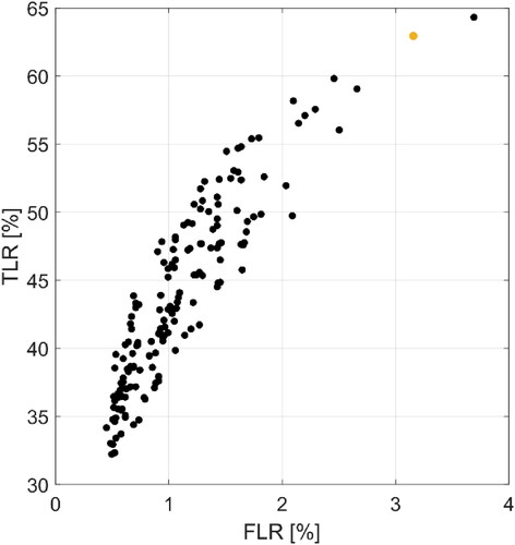
With this set of five waveform features, the optimal settings for each classifier were determined (as described in section Classifier Configuration). The optimal number of clusters (K) for the unsupervised classifiers was determined based on the ROC graphs as depicted in Figure 4b. This figure shows that a small number of clusters (K = 5) relates to a high FLR and low TLR, while for a higher number of clusters (K > 5), there is no clear correlation between cluster size and classifier performance. The HC classifier produces the same results for some of the clustering sizes (e.g., K = 5,10 or K = 15,20,25,30), indicating this classifier is inflexible. The selected settings for all classifiers are displayed in Table 3.

Figure 4. ROC graphs of supervised (a) and unsupervised (b) classifiers during the training phase of the D-01 data division. The ROC graphs of supervised classifiers are obtained by varying the discrimination threshold (see section Classifier Performance Assessment). The ROC graphs of the unsupervised classifiers are obtained by adjusting the number of clusters (K) as shown in the legend (b). Note the different limits on the axes.

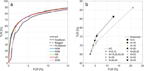
Table 3. Classifier settings, where $n$ is the size of the training dataset and $f$ the number of predictors.

Classifier	Settings
DT	Maximum number of splits = 100, Split criterion = Gini index
Bagged	Maximum number of splits = $n-1,$ Number of trees = 30
AdaBoost	Maximum number of splits = 100, Number of trees = 30, Learning rate = 0.1
RUSBoost	Maximum number of splits = 20, Number of trees = 30, Learning rate = 0.1, Class ratio = 1:1(:1).
ANN	Fully connected layers =1, Layer size = 10, Activation = ReLU, No regularization
NB	Predictor distribution = Gaussian
LD	Covariance structure = Full
SVM	Kernel function = Gaussian, Kernel scale = $\frac{1}{4}\sqrt{f},$ Box constrained level = 1
KNN	Number of neighbors k = 100, Distance metric = Euclidean
Kmedoids	Number of clusters $K$ = 15
HC	Number of clusters $K$ = 40, Linkage = farthest distance
Threshold	Classify as leads if MAX > 3000 counts, PPloc > 0.55, ww < 45 bins, PP > 0.24, and skew > 7. Classify as ocean if: MAX: 500-1500 counts, PPloc: 0.2-0.35, ww: 85-110 bins, PP < 0.1, and skew: 1.5-3.5. Else: sea ice (see Table 1 for abbreviations).

Based on the ROC graphs obtained during classifier configuration (Figure 4), the DT and SVM classifiers were excluded from the analysis since they produced lower AUC values (0.88 for SVM and 0.91 for DT) than the other supervised classifiers (all 0.94). Regarding the unsupervised classifiers, the Kmedoids classifier shows the best results as it consistently obtains higher TLR values than the HC classifier (Figure 4b). Therefore, the HC classifier was also excluded from further analyses.

Classification performances for winter data (D-01-D-03)

Classification performances obtained from the test cases with data from winter months are shown in Figures 5a and c. In Figure 5a, the best performances are connected to create an optimal front. Classifiers on this front obtain the highest TLRs for a given range of FLRs and are therefore perceived to outperform classifiers that are located away from the front. The best choice out of all classifiers that are located on the front depends on user preferences regarding the FLR. KNN, AdaBoost, and LD show the best results from the general performance test (D-01) as they are all located on the optimal front. However, there is little difference between these three and most other classifiers. The Threshold and Bagged classifiers are located away from the optimal front, indicating that they perform worse than the others. While RUSBoost is located on the optimal front with the highest TLR, it also achieved the highest FLR, which explains the lower overall accuracy (Figure 5c).

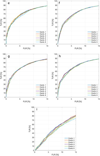
Figure 5. ROC graph showing classification performances for D-01, D-02, D-03 (a), and D-04 (b) (see description of test cases in Table 2). The marker style depicts the classifier, and the colors are used to differentiate between different study cases. The grey line in (a) shows the optimal front, while the grey line in (b) simply connects FLR = TLR = 0 and FLR = TLR = 100. Note the different limits on the axes. Overall classification accuracies [%] are shown in (c).

Most of the supervised learning classifiers do not suffer significantly when they are trained with data set from another year (D-02). Most classifiers are still part of the optimal front or very close to it. However, the Bagged and KNN classifiers perform poorly when trained with data set from another year. Lastly, the test concerning possible regional biasing (D-03) resulted in improved overall accuracy for most of the classifiers (up to 1.2%, Figure 5c). However, the performance of the supervised classifiers was reduced in terms of lead detection (Figure 5a). This indicates that these classifiers may perform slightly worse when they are trained with data sets from different study areas.

Classification performances for summer data (D-04)

All classifiers perform relatively poorly when applied to summer data (Figures 5b and c). Classifiers in the lower FLR range (<20%) produce very low TLRs (under detection): AdaBoost, Bagged, ANN, KNN, NB, and LD, while classifiers with a higher TLR also produce high FLRs (>40%; overdetection): RUSBoost, Kmedoids, and Threshold. All classifier performances are very close to the diagonal line in Figure 5b, indicating that the classifiers are not much better than random guessing. Especially, the Kmedoids and Threshold classifiers produce extremely low overall accuracies (Figure 5c).

Classification performance with additional open ocean class (D-05)

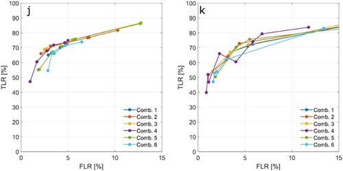
Finally, to allow for increased reliability of SSH estimation by the inclusion of open water samples, the classifiers were additionally assessed with consideration of this third class. When overall accuracy is considered, most classifiers do not suffer from the addition of the open ocean class (Figure 6a). Only the LD and Kmedoids classifiers perform significantly worse in the D-05 test case. However, regarding the distinction between leads and sea ice waveforms, all classifiers perform slightly worse (higher FLRs; Figure 6b). This effect is most pronounced for LD, NB, RUSBoost, and especially Kmedoid. The TwRs are relatively high for most classifiers except for LD and Kmedoids, which also produce very high FwRs. In all cases, the real FLRs, which compares both sea ice and ocean waveforms against leads (Figure 6b: dashed line + dot), are lower than when ocean data are excluded from this measure. This indicates that a negligible number of ocean waveforms are misclassified as leads.

Figure 6. Overall classification accuracies [%] for D-01 and D-05 (a), complemented by ROC graphs showing classification performances (b). The D-05 results are plotted in three ways: using the TLR and FLR that compare lead classifications to sea ice classifications (black) to allow direct comparison with the D-01 results, the actual TLR and FLR that compare lead classifications to sea ice and ocean classifications (dashed line + dot) and the TwR and FwR (red) that compare lead and ocean classifications to sea ice classifications. Note that the FwRs of LD and Kmedoids are outside plot limits.

Discussion

A wide range of classification methods was assessed for lead detection in the Arctic Ocean from Sentinel-3 satellite data. The classifiers were applied to SRAL data, while simultaneously sensed OLCI images were used for creating the ground truth data. For the latter, an automatic validation process was implemented that uses Kmeans image segmentation and along-track changes in radiance. This novel approach of using OLCI imagery was particularly useful because of the perfect temporal alignment between the two involved datasets. Disadvantages of using OLCI images are the dependency on illuminated and cloud-free conditions and the relatively low spatial resolution (compared to e.g., Operation Ice Bridge imagery (Dettmering et al. 2018)). Even though the spatial resolution of OLCI imagery equals the along-track resolution of SRAL data, a narrow lead may cause a specular SRAL waveform, while it would not be visible on the OLCI image. This would result in (seemingly) overdetection of leads, i.e., higher FLRs.

In total, nine supervising machine learning algorithms, two unsupervised machine learning algorithms, and a threshold classifier were applied to various test cases. This provides a comprehensive understanding of the performance of different classifiers and their applications. In this study, where the goal of lead detection is to improve the Arctic Ocean SSH estimation, a low FLR is treated as the most important classifier criterion. Misclassifications may result in large errors in the SSH estimation (see Appendix 3. Improving the Additional Open Ocean Classification, for an example). While the RUSBoost classifier produced results close to the optimal front for each winter test case (D-01-D-03; Figure 5a), its FLR values are very high compared to other classifiers. The RUSBoost classifier obtains such high FLR and TLR values because this algorithm opts to increase the correct classifications for the minor class (Seiffert et al. 2008), leading to overdetection of leads. The latter makes the classifier less suitable for SSH estimation. The Kmedoids classifier performed consistently well for the winter data (D-01-D-03). Because this is an unsupervised classifier, it can be directly applied to the data of interest, regardless of the available ground truth data. Hence, any consequences from temporal differences between training and testing data for the performance of supervised classifiers, do not apply to unsupervised classifiers. Therefore, if the ground truth data are unavailable for the testing area, using the Kmedoids classifier may be preferred. However, this classifier requires the user to manually assign waveform clusters to surface types, which is a disadvantage when a priori knowledge of the different waveform types belonging to certain classes is lacking. If sufficient ground truth is available, the supervised learning classifiers AdaBoost, LD, or ANN are preferred over the Kmedoids classifier, as their general performances were slightly better (up to 0.31%), and the classification does not require manual class assignment. Additionally, when large amounts of data are considered, the time complexity of the different classifiers favors the use of supervised classification. In the case of unsupervised classification, the time complexity is typically quadratically (Kmedoid) or cubically (HC) dependent on the number of observations (Bindra and Mishra 2017; Whittingham and Ashenden 2021), compared to a predominantly linear dependency for the supervised classifiers (e.g., Cai, He, and Han 2008; Deng et al. 2016; Fleizach and Fukushima 1998; Sani, Lei, and Neagu 2018). Finally, while the KNN classifier produced one of the best results in the general test case (D-01) and was only marginally affected by a regional bias (D-02), its performance worsened significantly when applied to data from another period (Figure 5c). This indicates that the KNN classifier could be very sensitive to a change in the dataset, making the classifier unpredictable. Almost all classifiers performed slightly worse when applied to data from another period than the training data, which argues for the consideration of a training data set that spans the full period of interest. Finally, it was shown that the Bagged classifier did not produce high enough TLRs in any of the winter test cases.

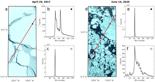
From the fourth test case (D-04) it appears that all classifiers perform poorly when applied to data from summer months (Figure 5b). This is likely related to the physical transformation of the sea ice during this period. Most of the altimetry return signals are specular, even when ground truth data suggest that they originate from sea ice (see Figure 7e). The presence of melt ponds on the surface of the sea ice may be the cause of this increase in specular returns during summer months. Unevenness in the color of the sea ice on the OLCI images (Figure 7d) may indicate melt ponds. This must however be confirmed with images from sensors with higher resolution. Additionally, more diffuse signals are returned from what appear to be leads based on the ground truth data (Figure 7f). This may be related to the presence of waves on widening leads, or the presence of separated ice floes smaller than the resolution of the OLCI images. The sole use of SAR waveform features for lead detection in summer months is deemed unsuitable and auxiliary information is required. For instance, in the study by Dawson et al. (2022) local variations in elevation were successfully used in addition to waveform features, to distinguish between SAR returns from leads and melt ponds. However, this does require preliminary retracking of the data before the classification and constrains the variety of leads that can be detected (Dawson et al. 2022). On another note, further research should show to what extent, reduced classifier performance impacts the uncertainty associated with SSH estimates from summer data. In this respect, it should be noted that the occurrence of sea ice, and thus leads, is significantly reduced in summer, resulting in more possibilities regarding SSH estimation from open water and reducing the need for accurate lead detection.

Figure 7. Example OLCI images with two typical SAR waveforms for a winter date (a–c) and a summer date (d–f). In both examples, the first waveform (b, e) belongs to sea ice and the second (c, f) to a lead according to the OLCI image, while in the summer case (d–f), the SAR waveforms were incorrectly classified as the opposite class by all classifiers.

Finally, to improve SSH estimation by reliable detection of open water areas, the addition of a third class is required. The addition of the open ocean class had little impact on the overall accuracy of most classifiers, except for LD and Kmedoids (Figure 6a). However, the performance of all classifiers decreased slightly in terms of lead detection (Figure 6b; TLR and FLR), while the impact on the Threshold and Bagged classifiers was the smallest. If one is purely interested in obtaining as many good water level measures as possible (considering TwR and FwR), the AdaBoost, Bagged and ANN classifiers perform best. The reduced performance of the Kmedoids classifier was associated with the fast increase in data, which cluttered the clusters and complicated manual class assignment. Moreover, the Threshold classifier performs poorly when TwR and FwR are concerned.

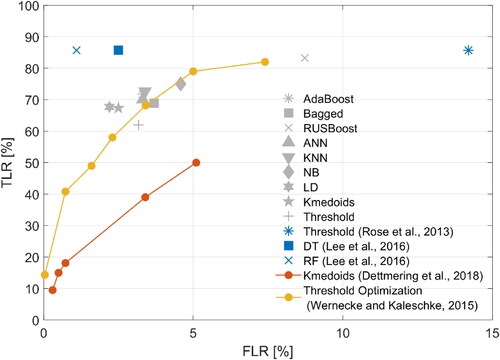
The results produced by this study were compared to results from other studies that tested different classification methods for lead detection from altimetry (Figure 8). However, caution is advised when comparing the classifier performances found in different studies. Differences in input data (e.g., SAR or conventional radar, different study dates or study areas), different settings for the classifiers, or different methods for ground truth data generation, impact the obtained classifier performances. For instance, Lee et al. (2016) applied two tree-based supervised machine learning classifiers to SAR altimetry data from CryoSat-2: DT and Random Forest (RF). The obtained classification results show extremely high accuracies and high TLR values compared to the results obtained in this paper. However, they tested their classifiers using only 239 waveforms, hence the classifiers may have been overfitted to this small dataset. Their findings show that the ensemble tree classifier (RF in their case) outperforms the DT classifier, which agrees with the findings presented here. Moreover, Dettmering et al. (2018) applied the unsupervised Kmedoids classifier to Cryo Sat-2 SAR altimetry data and used images from the NASA Operation Ice Bridge mission for validation. They obtained TLRs that were significantly lower than those produced by the Kmedoids classifier in this study. This may be because the resolution of the images from Operation Ice Bridge is 1 m (Dettmering et al. 2018), compared to the 300 m along-track resolution of CryoSat-2. This difference most likely resulted in the underdetection of leads from the altimeter data. Furthermore, Wernecke and Kaleschke (2015) classified CryoSat-2 data with threshold optimization, using MODIS images for validation. Their TLRs and FLRs are comparable to the results from this study, however, they only validated the classification with data from the Beaufort Sea.

Figure 8. ROC graphs showing classification results from previous studies and general performance (D-01) results obtained in this study.

Where the comparison of classifier performances presented by prior studies may be misleading, this study provides a comprehensive assessment of the relative classifier performances. Nevertheless, there are more classifiers that could be applied to lead detection in the Arctic. For instance, the results from Lee et al. (2016) suggest that the RF classifier performs well, which has not been tested in this study. Furthermore, the use of OLCI images for validation appeared very useful because of their perfect temporal alignment with the SRAL data. However, while the generation of ground truth data has been largely automated in this study, a manual check was required to reject images that were deteriorated by small clouds. This process is time-consuming and future studies may benefit from an improved algorithm for cloud rejection that would also detect small and thin clouds, allowing more ground truth data to be generated. A solution may be the combination of OLCI images and Sea and Land Surface Temperature Radiometer (SLSTR) data, which have recently been used for cloud detection (Fernandez-Moran et al. 2021). This synergy could also be exploited to better distinguish between leads and melt ponds. Likewise, for specific test cases or when additional (sub)classes are considered, the classification may benefit from a different/extended set of waveform features. For instance, it was found that sea ice waveforms sometimes resemble open ocean waveforms (see Appendix 3. Improving the Additional Open Ocean Classification), which would cause large errors in the SSH estimation. For most of the data, a clear regional separation between sea ice and the open ocean can be assumed. Therefore, the initial set of waveform features may be extended by a certain along-track history parameter. For instance, the addition of the moving standard deviation of the pulse peakiness (see Table 1) appeared to significantly improve the three-class classification performances (Appendix 3. Improving the Additional Open Ocean Classification). Finally, it should be acknowledged that the predictors used in this study are to some degree correlated with each other (see Appendix 4. Predictor Correlation). While this is something that should generally be avoided in any statistical model (including classifiers) (Blalock 1963), Figure A4.1 shows that the correlation within the set of predictors is largely consistent across different data divisions and is therefore expected to have a limited effect on the quality of the classifiers.

Conclusions

This paper provides a thorough assessment of twelve different waveform classification methods, applied to Sentinel-3 SRAL data. Here, the perfect temporal alignment between SRAL and OLCI data was successfully exploited for generating the ground truth data. In addition to assessing the general classifier performance, the classifiers were applied to different test cases to analyze the impact of possible regional or temporal biasing and the impact of additional classes.

It was shown that all classifiers performed relatively well on data from March and April (2017–2020). Overall, the AdaBoost and ANN classifiers showed the most robust results throughout the analysis. However, supervised learning requires labeled training data, and thus ground truth data must be available. This study showed that the usage of training data from another study area or a different year slightly worsens the performance of some classifiers, hence the use of a comprehensive training dataset is recommended. Alternatively, the unsupervised machine learning Kmedoids classifier does not require the ground truth data and consistently showed excellent results but performed poorly when tracks that (partly) cover open ocean were considered. Additionally, the interpretation of classifications by Kmedoids is sensitive to differences in user knowledge. Moreover, if large amounts of data are considered, the supervised classifiers may be preferred over unsupervised classifiers as they typically have lower time complexities. Finally, the thresholding method performs worse than the machine learning-based methods yet may still be preferred due to its simplicity in application.

Disclosure statement

No potential conflict of interest was reported by the authors.

Data availability statement

Sentinel-3 OLCI imagery and SRAL data are available through the Earth Observation Portal from EUMETSAT (https://eoportal.eumetsat.int).

Additional information

Funding

This work is part of the research program FAST4Nl with project number ALWPP.2017.001, which is (partly) financed by The Netherlands Organisation for Scientific Research (NWO).

Appendix 1.

Definition of Threshold Classifier

For the Threshold classifier, the threshold values were determined by solving an optimization problem. For this, the distribution of the waveform features was studied on a class-by-class basis. For each feature, a range of thresholds was empirically determined that would separate most leads from sea ice waveforms. This resulted in the following ranges; MAX: 3000–7000, skew: 7–8, PP: 0.15–0.35, PPloc: 0.5–0.7, and ww: 25–50. Note that this only involves the five features with the best predictive capacity as was determined in Appendix 2. Tuning of Classifiers. Subsequently, 200 random combinations of thresholds within these ranges were created and applied to the data (Wernecke and Kaleschke 2015). The result of this random search is analyzed based on the produced TLR and FLR (Figure A1.1). The final set of thresholds was chosen such that the total number of misclassifications was minimized. Waveforms are classified as leads when: MAX > 3000 counts, PPloc > 0.55, ww < 45 bins, PP > 0.24, and skew > 7. For the D-05 experiment, the thresholds for ocean classes were determined as follows: 500 > MAX > 1500 counts, 0.2 > PPloc 0.35, 85 > ww > 110 bins, PP < 0.1, and 1.5 > skew > 3.5. The remaining data were classified as sea ice.

Figure A1. 1. ROC graph showing the results of the random search of thresholding values for lead classification. The orange point depicts the final choice of the thresholding values used in the paper.

Appendix 2.

Tuning of Classifiers

As described in section Classifier Configuration, the classification potential of individual waveform features was studied. For each considered classifier, the resulting accuracies are given in Table A2.1. The produced accuracies are generally high, with most of the waveform features producing more than 80% accuracy for most of the classifiers. However, the unsupervised learning classifiers (Kmedoids and HC) achieved substantially lower accuracies when using LeW, PPL, PPR, and NrPeaks. The HC classifier also did not perform well when using kurtosis. It was found that using WW, PP, PPloc, skewness, and MAX, produces high accuracy for all classifiers. Though TeW has achieved a high average accuracy, it has not been selected due to the relatively low accuracy produced by the Kmedoids classifier. Additionally, most of the supervised learning classifiers produced very similar results when using NrPeaks (79.8%). However, all classifiers that produced this accuracy predicted all of the waveforms to be sea ice, i.e., obtained a TLR of 0%. Because NrPeaks can only have discrete integer values, it is not a suitable feature for machine learning algorithms. Previous studies which used NrPeaks as a predictor, were thresholding-based classifications (e.g., Bij de Vaate et al., 2021; Schulz and Naeije 2018).

Table A2.1. Training accuracies [%] of classifiers trained with a single predictor. The shaded rows indicate the parameters that were selected for this paper.

	Ada-Boost	Bagged	KNN	SVM	DT	NB	LD	ANN	RUS-Boost	Kmedoids	HC	Average
MAX	88.76	88.76	88.84	88.96	88.18	88.92	88.93	88.92	88.76	83.41	82.86	87.85
Kurt	87.84	87.78	87.83	88.06	87.06	88.07	88.05	88.07	87.85	86.57	49.50	84.55
Skew	89.04	89.05	88.95	89.08	88.40	89.05	89.06	89.06	89.00	87.59	88.39	88.81
PP	90.79	90.82	90.90	91.01	90.25	90.97	90.98	90.98	90.82	90.68	90.67	90.82
WW	91.02	91.00	91.05	91.10	90.99	91.10	91.10	91.10	91.03	90.93	90.84	91.03
LeW	85.82	85.82	85.82	85.82	85.82	79.88	85.82	85.82	85.82	20.91	28.46	75.14
TeW	88.38	88.38	88.38	88.38	88.38	88.38	88.38	88.38	88.38	71.28	86.45	86.79
sigma0	87.27	99.43	87.15	87.19	87.82	86.02	86.06	87.21	84.15	69.23	64.41	84.18
PPL	86.35	86.45	86.50	86.52	85.65	86.52	86.55	86.47	86.38	43.60	20.18	77.30
PPR	87.53	87.56	87.72	87.79	86.96	87.76	87.80	87.82	87.61	70.48	20.17	80.58
PPloc	90.32	90.48	90.41	90.49	89.89	90.49	90.49	90.46	90.50	89.79	90.26	90.34
NrPeaks	79.80	79.80	79.80	79.80	79.80	79.80	79.80	79.80	44.30	59.10	70.22	73.80

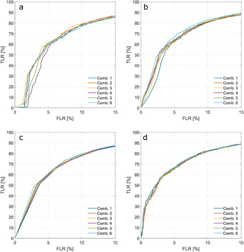
The sensitivity to the addition of more predictors to the initial set of five (MAX, skew, PP, ww, PPloc) was assessed by a comparison of the produced ROC graphs (Figure A2.1). Six possible combinations of the features were tested (Table A2.2). Here, the NrPeaks was excluded completely.

Table A2.2. Combinations of waveform features which were used in this analysis.

Combination	Waveform Features
Combination 1	MAX, skew, PP, ww, and PPloc
Combination 2	MAX, skew, PP, ww, PPloc, and kurt
Combination 3	MAX, skew, PP, ww, PPloc, and TeW
Combination 4	MAX, skew, PP, ww, PPloc, and PPR
Combination 5	MAX, skew, PP, ww, PPloc, kurt, TeW, and PPR
Combination 6	MAX, skew, PP, ww, PPloc, kurt, TeW, PPR, LeW, sigma0, and PPL

From Figure A2.1, it appears that for most classifiers, the addition of predictors does not have a significant effect on classifier performance. The largest effects are observed for DT and SVM (Figure A2.1a/i), but this concerns reduced performance when more predictors are included. Adaboost and Bagged (Figure A2.1b/c) may benefit to some extent from the larger set of predictors, although this is mostly restricted to the far low FLR range (<4%). In addition, both unsupervised classifiers appear to benefit from the addition of kurt, TeW and or PPR, although the effect is small.

Figure A2. 1. ROC graphs of supervised learning algorithms for different waveform feature combinations (see Table A2.2): DT (a), AdaBoost (b), Bagged (c), RUSBoost (d), ANN (e), KNN (f), LD (g), NB (h) and SVM (i), Kmedoids (j) and HC (k).

Appendix 3.

Improving the Additional Open Ocean Classification

Since the main goal of this paper is to improve the detection of leads, classifier settings and selection of waveform features have been optimized with the focus on the distinction between leads and sea ice. However, when one is interested in processing satellite tracks that may include SAR returns from the open ocean, the classification may be further optimized. As can be seen in Figure A3.1a, the misclassification of sea ice returns as open ocean (isolated black dots between 70 and 77^oN) can result in large SSH errors. To prevent these misclassifications, one could opt for the addition of a certain along-track history parameter that combines values from neighboring samples (referred to as test case D-05h).

Figure A3. 1. An example of an along-track SSH series referenced to DTU18-MSS (Sentinel-3B track from November 5, 2021) obtained by the AdaBoost classifier and retracked by fitting the SAMOSA model (Dinardo et al. 2018; Ray et al. 2015) (a). Along-track PP and moving standard deviation of the along-track PP (b).

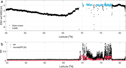
Here, this history parameter was defined as the moving standard deviation of the PP over 25 neighboring samples (see Figure A3.1b). In the Threshold classifier, the following condition was added for the ocean class: movstd(PP, 25) < 0.01.

Figure A3. 2. Overall classification accuracies [%] for D-05 and D-05h (a), complemented by ROC graphs showing classification performances (b). The D-05(h) results are plotted in two ways: the actual TLR/FLR where lead classes are compared to ocean and ice combined (black/grey) and the TwR/FwR (red/orange) that combines the water classes (ocean and leads). Note that the red/orange markers for AdaBoost and ANN overlap.

The addition of the history feature significantly improved the classification of both ocean and lead waveforms (Figure A3.2). All performance measures improved, but the effect on the TwR and FwR was the strongest, in particular for the Threshold and Kmedoids classifier. Note that in this study, the ocean data were added as a single separate track. The addition of a history feature would likely not improve the classification of consecutive ocean and sea ice data points. However, most ocean and sea ice data are well separated.

Appendix 4.

Predictor correlation

A common issue to occur in multivariate analyses is multicollinearity. This phenomenon – where one or more predictors are linearly related – can lead to biased estimation and may cause the trained model to be unstable (Yoo et al. 2014). Ideally, the predictor variables would be chosen in such a way that the correlation between predictors (waveform features) is minimized, yet the correlation with the response variable (class in this case) is large. To test the impact of multicollinearity in the study case described in this paper, Pearson correlation coefficients are calculated for each predictor pair and Kendall correlation coefficients for each predictor-response pair. This is done for all data divisions as described in the paper (Figure A4.1).

Figure A4. 1. Absolute correlation coefficients of all predictor pairs and the correlation coefficient between each predictor and the response variable (Class): for the D-01 dataset (a), the D-02 training (b) and testing dataset (c), the D-03 training (d) and testing dataset (e), the D-04 summer data (f) and the D-05 set including ocean data (g). The dots indicate the features that were used in this study.

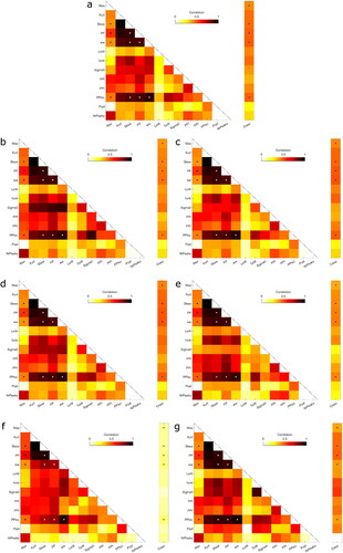
Four of five predictors used in the study are highly correlated: skew, PP, ww, and PPloc (Figure A4.1a). However, these features are all directly dependent on the shape of the waveform and therefore the correlation is in this case deemed inevitable. Nevertheless, if the correlation among predictor variables is consistent across the data divisions that the trained model is applied to, multicollinearity does not necessarily degrade classifier performance (Kutner et al. 2018). This mainly concerns the D-02 and D-03 test cases (Table 2). From Figure A4.1b/c and d/e, it appears that the correlation between the considered predictors remains consistent, regardless of differences in the study area or sensing period. This does not apply to all predictors (e.g., sigma0). The distinct difference between Figure A4.1f and other subfigures suggests that a classifier trained with winter data should not be applied to classify summer data. In addition, the low correlation between all predictors and the response variable (Figure A4.1f) emphasizes the poor potential in summer surface classifications based solely on altimetry data.

Appendix 5.

List of Abbreviations

Table A5.1. Abbreviations used in this paper.

Abbreviation	Explanation
SSH	Sea surface height
SAR	Synthetic Aperture Radar
SRAL	Synthetic Aperture Radar Altimeter
OLCI	Ocean and Land Color Instrument
SWH	Significant Wave Height
MAX	Maximum power (waveform feature)
Kurt	Kurtosis (waveform feature)
Skew	Skewness (waveform feature)
PP	Pulse Peakiness (waveform feature)
Ww	Waveform width (waveform feature)
LeW	Leading edge width (waveform feature)
TeW	Trailing edge width (waveform feature)
Sigma0	Backscatter coefficient (waveform feature)
PPL	Pulse Peakiness Left (waveform feature)
PPR	Pulse Peakiness Right (waveform feature)
Pploc	Local Pulse Peakiness (waveform feature)
NrPeaks	Number of peaks (waveform feature)
DT	Decision tree (classification method)
Bagged	Bootstrap Aggregation (classification method)
AdaBoost	Adaptive Boosting (classification method)
RUSBoost	Random undersampling boosting (classification method)
ANN	Artificial Neural Network (classification method)
NB	Naïve Bayes (classification method)
LD	Linear Discriminant (classification method)
SVM	Support Vector Machine (classification method)
KNN	K-Nearest Neighbors (classification method)
Kmedoids	K-Medoids clustering (classification method)
HC	Hierarchical clustering (classification method)
TLR	True Lead Rate
FLR	False Lead Rate
TwR	True water Rate
FwR	False water Rate
ROC	Receiver Operating Characteristics
AUC	Area Under the Curve
RF	Random Forest (classification method)

References

- Blalock, H. M. Jr., 1963. Correlated independent variables: The problem of multicollinearity. Social Forces 42 (2):233–7.
- Breiman, L. 1996. Bagging predictors. Machine Learning 24 (2):123–40.
- Cai, D., X. He, and J. Han. 2008. Training linear discriminant analysis in linear time. 2008 IEEE 24th international conference on data engineering, 209–217.
- Cazenave, A., B. Hamlington, M. Horwath, V. R. Barletta, J. Benveniste, D. Chambers, P. Döll, A. E. Hogg, J. F. Legeais, M. Merrifield, et al. 2019. Observational requirements for long-term monitoring of the global mean sea level and its components over the altimetry era. Frontiers in Marine Science 6:582.
- Collecte Localisation Satellites (CLS). 2011. Surface Topography Mission (STM) SRAL/MWR L2 Algorithms Definition, Accuracy and Specification.
- Dawson, G., J. Landy, M. Tsamados, A. S. Komarov, S. Howell, H. Heorton, and T. Krumpen. 2022. A 10-year record of Arctic summer sea ice freeboard from CryoSat-2. Remote Sensing of Environment 268:112744.
- Deng, Z., X. Zhu, D. Cheng, M. Zong, and S. Zhang. 2016. Efficient kNN classification algorithm for big data. Neurocomputing 195:143–8.
- Dettmering, D., A. Wynne, F. L. Müller, M. Passaro, and F. Seitz. 2018. Lead detection in polar oceans-a comparison of different classification methods for Cryosat-2 SAR data. Remote Sensing 10 (8)1190.
- Dinardo, S., L. Fenoglio-Marc, C. Buchhaupt, M. Becker, R. Scharroo, M. J. Fernandes, and J. Benveniste. 2018. Coastal SAR and PLRM altimetry in German Bight and West Baltic Sea. Advances in Space Research 62 (6):1371–404.
- Donlon, C., B. Berruti, A. Buongiorno, M.-H. Ferreira, P. Féménias, J. Frerick, P. Goryl, U. Klein, H. Laur, C. Mavrocordatos, et al. 2012. The global monitoring for environment and security (GMES) sentinel-3 mission. Remote Sensing of Environment 120:37–57.
- Fenoglio-Marc, F., S. Dinardo, R. Scharroo, A. Roland, M. Dutour Sikiric, B. Lucas, M. Becker, J. Benveniste, and R. Weiss. 2015. The German Bight: A validation of CryoSat-2 altimeter data in SAR mode. Advances in Space Research 55 (11):2641–56.
- Fernandez-Moran, R., L. Gómez-Chova, L. Alonso, G. Mateo-García, and D. López-Puigdollers. 2021. Towards a novel approach for Sentinel-3 synergistic OLCI/SLSTR cloud and cloud shadow detection based on stereo cloud-top height estimation. ISPRS Journal of Photogrammetry and Remote Sensing 181:238–53.
- Flach, P. A. 2016. ROC analysis. In Encyclopedia of machine learning and data mining. Boston, USA: Springer.
- Fleizach, C, and S. Fukushima. 1998. A naive bayes classifier on 1998 JDD cup.
- Freund, Y., and R. Schapire. 1999. A short introduction to boosting. Journal of Japanese Society for Artificial Intelligence 14 (5):771–80.
- Friedman, N., D. Geiger, and M. Goldszmidt. 1997. Bayesian Network Classifiers. Machine Learning 29 (2/3):131–63.
- Grossi, E., and B. Massimo. 2007. Introduction to artificial neural networks. European Journal of gastroenterology & hepatology 19 (12):1046–54.
- Hamada, M., Y. Kanat, and A. Adejor. 2019. Sea ice drift in the Arctic since the 1950s. International Journal of Innovative Technology and Exploring Engineering 2:1016–9.
- Hastie, T., R. Tibshirani, and J. Friedman. 2009. The elements of statistical learning: Data mining, inference, and prediction. New York, USA: Springer.
- IPCC. 2021. Climate Change 2021: The Physical Science Basis. Contribution of Working Group I to the Sixth Assessment Report of the Intergovernmental Panel on Climate Change, eds. V. Masson-Delmotte, P. Zhai, A. Pirani, S.L. Connors, C. Péan, S. Berger, N. Caud, Y. Chen, L. Goldfarb, M.I. Gomis, M. Huang, K. Leitzell, E. Lonnoy, J.B.R. Matthews, T.K. Maycock, T. Waterfield, O. Yelekçi, R. Yu, and B. Zhou. Cambridge, UK: Cambridge University Press. In Press.
- Kaufman, L., and P. Rousseeuw. 1987. Clustering by means of medoids. Statistical data analysis based L1 norm related methods, 405–16. Basel, Switzerland: Birkhäuser Verlag.
- Kutner, M. H., C. J. Nachtsheim, J. Neter, and W. W. Li. 2005. Applied linear statistical models. New York, USA: McGraw Hill Irwin.
- Kwok, R. 2018. Arctic sea ice thickness, volume, and multiyear ice coverage: Losses and coupled variability (1958–2018). Environmental Research Letters 13 (10):105005.
- Laxon, S. 1994. Sea ice altimeter processing scheme at the EODC. International Journal of Remote Sensing 15 (4):915–24. doi:10.1080/01431169408954124.
- Laxon, S. W., K. A. Giles, A. L. Ridout, D. J. Wingham, R. Willatt, R. Cullen, R. Kwok, A. Schweiger, J. Zhang, C. Haas, et al. 2013. CryoSat‐2 estimates of Arctic sea ice thickness and volume. Geophysical Research Letters 40 (4):732–7.
- Lee, S., J. Im, J. Kim, M. Kim, M. Shin, H. Kim, and L. Quackenbush. 2016. Arctic sea ice thickness estimation from CryoSat-2 Satellite Data using machine learning-based lead detection. Remote Sensing 8 (9):698.
- Müller, F. L., D. Dettmering, W. Bosch, and F. Seitz. 2017. Monitoring the arctic seas: How satellite altimetry can be used to detect open water in sea-ice regions. Remote Sensing 9 (6):551.
- Murtagh, F., and P. Contreras. 2012. Algorithms for hierarchical clustering: An overview. WIREs Data Mining and Knowledge Discovery 2 (1):86–97.
- Peacock, N., and S. Laxon. 2004. Sea surface height determination in the Arctic Ocean from ERS altimetry. Journal of Geophysical Research 109 (C7):1–14.
- Poisson, J., G. Quartly, A. Kurekin, P. Thibaut, D. Hoang, and F. Nencioli. 2018. Development of an ENVISAT altimetry processor providing sea level continuity between open ocean and arctic leads. IEEE Transactions on Geoscience and Remote Sensing 56 (9):5299–319.
- Qin, A., S. Shi, P. Suganthan, and M. Loog. 2005. Enhanced direct linear discriminant analysis for feature extraction on high dimensional data. Proceedings of the National Conference on Artificial Intelligence 2, 851–5.
- Quartly, G. D., E. Rinne, M. Passaro, O. B. Andersen, S. Dinardo, S. Fleury, A. Guillot, S. Hendricks, A. A. Kurekin, F. L. Müller, et al. 2019. Retrieving sea level and freeboard in the Arctic: A review of current radar altimetry methodologies and future perspectives. Remote Sensing 11 (7)881.
- Quinlan, J. 1986. Induction of decision trees. Machine Learning 1 (1):81–106.
- Raney, R. 1998. The delay/doppler radar altimeter. IEEE Transactions on Geoscience and Remote Sensing 36 (5):1578–88.
- Ray, C., C. Martin-Puig, M. P. Clarizia, G. Ruffini, S. Dinardo, C. Gommenginger, and J. Benveniste. 2015. SAR altimeter backscattered waveform model. IEEE Transactions on Geoscience and Remote Sensing 53 (2):911–9.
- Ricker, R., S. Hendricks, V. Helm, H. Skourup, and M. Davidson. 2014. Sensitivity of CryoSat-2 Arctic sea-ice freeboard and thickness on radar-waveform interpretation. The Cryosphere 8 (4):1607–22.
- Rose, S., R. Forsberg, and L. Pedersen. 2013. Measurements of sea ice by satellite and airborne altimetry, PhD diss., DTU Space.
- Rose, S. K., O. B. Andersen, M. Passaro, C. A. Ludwigsen, and C. Schwatke. 2019. Arctic Ocean sea level record from the complete radar altimetry era: 1991–2018. Remote Sensing 11 (14):1672.
- Sani, H. M, C. Lei, and D. Neagu. 2018. Computational complexity analysis of decision tree algorithms. In International Conference on Innovative Techniques and Applications of Artificial Intelligence. Springer.
- Schulz, A. T., and M. Naeije. 2018. SAR Retracking in the Arctic: Development of a year-round retrackers system. Advances in Space Research 62 (6):1292–306.
- Seiffert, C., T. M. Khoshgoftaar, J. Van Hulse, and A. Napolitano. 2008. RUSBoost: Improving classification performance when training data is skewed. Presented at 2008 19th International Conference on Pattern Recognition, IEEE.
- Savas, C., and F. Dovis. 2019. The impact of different kernel functions on the performance of scintillation detection based on support vector machines. Sensors 19 (23):5219.
- Shen, X., J. Zhang, X. Zhang, J. Meng, and C. Ke. 2017. Sea ice classification Using Cryosat-2 altimeter data by optimal classifier-feature assembly. IEEE Geoscience and Remote Sensing Letters 14 (11):1948–52.
- Shu, S., X. Zhou, X. Shen, Z. Liu, Z. Tang, H. Li, C. Ke, and J. Li. 2020. Discrimination of different sea ice types from CryoSat-2 satellite data using an Object-based Random Forest (ORF). Marine Geodesy 43 (3):213–33.
- Tangirala, S. 2020. Evaluating the impact of GINI index and information gain on classification using decision tree classifier algorithm. International Journal of Advanced Computer Science and Applications 11 (2):612–9.
- Timmermans, B. W., C. P. Gommenginger, G. Dodet, and J. R. Bidlot. 2020. Global wave height trends and variability from new multimission satellite altimeter products, reanalyses, and wave buoys. Geophysical Research Letters 47 (9):e2019GL086880.
- Wernecke, A., and L. Kaleschke. 2015. Lead detection in Arctic sea ice from CryoSat-2: Quality assessment, lead area fraction and width distribution. The Cryosphere 9 (5):1955–68.
- Wingham, D., C. Francis, S. Baker, C. Bouzinac, D. Brockley, R. de Cullen, P. Chateau-Thierry, S. Laxon, U. Mallow, C. Mavrocordatos, et al. 2006. CryoSat: A mission to determine the fluctuations in Earth’s land and marine ice fields. Advances in Space Research 37 (4):841–71.
- Whittingham, H, and S. K. Ashenden. 2021. Hit discovery. In The Era of Artificial Intelligence, Machine Learning, and Data Science in the Pharmaceutical Industry. San Diego, USA: Academic Press.
- Xu, L., J. Li, and A. Brenning. 2014. A comparative study of different classification techniques for marine oil spill identification using RADARSAT-1 imagery. Remote Sensing of Environment 141:14–23. rse.2013.10.012.
- Yoo, W., R. Mayberry, S. Bae, K. Singh, Q. P. He, and J. W. Lillard. Jr. 2014. A study of effects of multicollinearity in the multivariable analysis. International Journal of applied science and technology 4 (5):9–19.
- Zakharova, E. A., S. Fleury, K. Guerreiro, S. Willmes, F. Rémy, A. V. Kouraev, and G. Heinemann. 2015. Sea ice leads detection using SARAL/AltiKa altimeter. Marine Geodesy 38 (sup1):522–33.
- Zhang, H., T. W. Weng, P. Y. Chen, C. J. Hsieh, and L. Daniel. 2018. Efficient neural network robustness certification with general activation functions. Advances in neural information processing systems 31: 4944–4953.
- Zygmuntowska, M., K. Khvorostovsky, V. Helm, and S. Sandven. 2013. Waveform classification of airborne synthetic aperture radar altimeter over Arctic sea ice. The Cryosphere 7 (4):1315–24.