Aggregation Methods Using Bathymetry Sources of Differing Subjective Reliabilities for Navigation Mapping

Abstract

When planning for ship navigation or compiling data for a bathymetry map, the navigator or mapper uses many different sources of bathymetry information and navigation hazards. The quality of these sources is inconsistent in general, however, making it challenging to provide a coherent picture for planning. Here, we describe an approach for consistent planning/mapping that uses a combination of soft computing and Bayesian estimation. The case study used to exercise this system involves NOAA Electronic Nautical Charts for an area in the Chesapeake Bay. We first interpolate each set of irregularly spaced soundings to gridded versions of each point-cloud set. Each of these intermediate grids is then aggregated into a fused bathymetric realization using order weighted averaging (OWA) to provide the weights for each source based on their subjective reliabilities. The OWA allows for fusion informed by the user’s subjective risk allowed in the reconstruction of the seafloor surface and provides quantitative methods to generate, use, and record subjective reliability weights. Each sounding point that went into the bathymetry estimate is then categorized as “no-go,” “caution,” or “go” status. Reliability estimates are reused for weighted Bayesian categorization of each output grid cell to compute the navigable surface.

Keywords:

• Bathymetry fusion
• Bayesian categorical estimation
• navigation risk
• order weighted average

Introduction

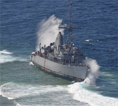
Effective and safe ship transit is of great concern to the development of products for navigational decision making. It is well-known that mistakes or imprecision in navigation charts have led to numerous shipwrecks. A review of Canadian, United States, and European shipwreck data (Bakdi et al. 2019) reports a total of over 100,000 maritime accidents during various periods over the 2000 to 2019 era. This includes cargo, military, and passenger transport ships. The grounding of the USS Guardian (Figure 1) is one recent example (Walhey 2013).

Figure 1. Grounding of the USS Guardian on the Tubbataha Reef (130 km southeast of Palawan, Philippines) in January 2013 (US Navy photo, public domain).

Over 90% of worldwide commerce uses shipping (Naevestad et al. 2019), often from ports located on the major rivers of the world. Where major rivers flow into the ocean there are many navigation problems. For example, the Columbia River of the western United States has the Columbia Bar, a shifting sandbar that makes the river’s mouth one of the most hazardous stretches of water to navigate in the world (Saddler 2006). Since 1792, approximately 2,000 large ships have sunk in and around the Columbia Bar, and because of the danger as well as the numerous shipwrecks the mouth of the Columbia River, this location has acquired a reputation worldwide as the graveyard of the Pacific (Wilma 2006).

The most important task of a ship navigator is to decide how to safely traverse the water surface between start and ending points of a ship’s course. While there are multiple factors related to safe navigation (e.g. avoidance of hazardous weather, areas of civil unrest, etc.), in this article, we use the term “safe navigation” to mean that the vessel does not make contact with the seafloor or underwater obstructions, where the depth of the keel dictates the shallowest depth that it can navigate (Calder 2015; Gilardoni and Presedo 2017).

An experienced navigator uses multiple sources of information for multicriteria decision making and forms a mental-model of safe navigation areas based on the location of soundings (geospatial points on a chart attributed with water depth) as well as obstruction or “hazard” locations to avoid (Cutler 2003). Part of the rationale for this mental processing is that point representations of seafloor depth and hazards on Electronic Navigation Charts (ENC; International Hydrographic Office 2000) are sparse geospatially. Soundings are quantitative but often lack information regarding the uncertainty of the depth, such as one standard deviation, an interval, a percentage of water depth or, as defined by the International Hydrographic Organization (IHO), a Category Zone of Confidence (CATZOC) (International Hydrographic Organization 2020). Hazards, however, have a qualitative aspect on charts. Cartographers generating the chart provide qualitative identification of the hazard using symbols that map the location on the chart and linguistic labels for each symbol (e.g. “shipwreck,” “sounding doubtful,” “rocks,” “value of sounding” (VALSOU), etc.) to identify the hazard type.

A navigator can judge that information sources have differing degrees of reliability based on the nature of the charts being used, the configuration of the soundings and contours, the known or estimated character of the seafloor, the age of the data, and so forth (Calder 2015). Such human-in-the-loop judgment is becoming even more important as community-based bathymetry collection becomes further developed (Calder et al. 2020), machine learning-based assessments from imagery become implemented (Chénier et al. 2020), source type and technology used to collect the data become attributed to digital bathymetry data as well as subsequent charts (Calder 2015, Weatherall et al. 2015; International Hydrographic Office 2019; EMODnet Bathymetry Consortium 2020; Jakobsson et al. 2020), and CATZOC attributions are assessed more fully in ENCs (International Hydrographic Organization 2020). Thus, the critical aspects of this human-based production of a navigation plan are (a) forming a believable forecast of seafloor depth contours in the areas between the soundings and (b) doing so using optimistic and pessimistic outlooks of what the information means for keel clearance as influenced by information sparsity and reliability. Although automated and objective means for multicriteria route planning and navigation risk-evaluation are now being proposed in the literature (Bakdi et al. 2019; Jeong et al. 2019; Kastrisios et al. 2020), a human still makes the final judgment for execution of the route and will assess the reliability of all information presented through human-in-the-loop processes.

In this article, we describe a hybrid-framework using both soft computing and quantitative methodologies that provide an approach for navigation planning. Our objective is to develop this framework through application of ordered weighted averaging (OWA) (Yager 1988; Beliakov, Pradera, and Calvo 2007) and Dirichlet categorical estimation (Gelman et al. 2013) subprocesses, respectively. The use of the OWA provides a means for allowing the human-in-the-loop judgment of reliability of the information sources and attitudinal risk tolerance than can be used in the quantitative Bayesian estimate of navigation risk category. This process provides a chart of clearly defined areas for safe or unsafe navigation as well as fuzzy areas in between where it may be safe or unsafe for navigation by mapping areas that are “go,” “no-go,” and “caution” areas, respectively. Another reason for the use of the OWA, a fuzzy logic stage, is significantly reduced computation costs versus a strict Bayesian approach for the steps of the process involving injection of linguistic/subjective/nonnumerical knowledge into the analysis.

Section “Approach” of this article presents the overall approach. The OWA is formally introduced. The section provides simple examples of how to use the OWA with a simple bathymetric test example. The OWA is further developed to show how human assessed reliability can be used for the fusion process and how the reliabilities then are reused in the Bayesian process, respectively. Section “Case study setup” introduces a case study of using this framework with ENC data in the Chesapeake Bay area. An overview of the data and computational implementations are discussed. Section “Results” provides results of the test case for two example keel depths, showing how the reliabilities assessments, attitudinal risk tolerance, and number of points used affect the results. Sections “Discussion” and “Summary” provide discussion and summary, respectively.

Approach

The approach here is to allow for a construction of the seafloor surface from the various sources using the OWA and Bayesian techniques. Specifically, the problem being solved is the inconsistency in charted soundings and information due to differences in compilation and generalization. The OWA is needed to generate “safe” realisations, and then, the Bayesian categorical estimation is used to fuse these into an estimated navigation category. Deeper or shallower estimates of depths can be based on parameters that could be adjusted to reflect the opinion of expert observers, environmental events within the area, the current tactical situation, and other factors. The use of this combined approach enables the use of these human-based and other qualitative factors within a recordable and quantitative framework. This framework also allows for record keeping of these qualitative factors so these judgments are inspectable and computations are reproducible.

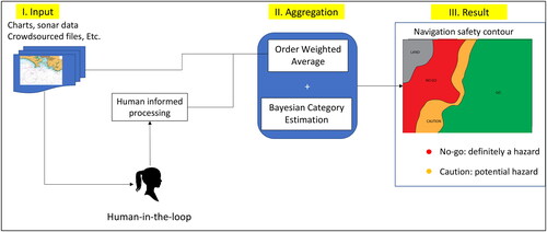
Overall, irregularly spaced soundings are used as input, which then undergo aggregation and categorical processing steps; the output is gridded map displaying differing navigation categories (Figure 2). We use charted soundings from ENC data for this input data. We assume that the typical end-user would obtain such information from ENC products rather than accessing databases with multibeam or single beam soundings for input (although use of such database information is permissible in this framework) due to volume of such data and level of expertise required to process it correctly. Here, only the soundings as they appear in the “SOUNDG” layer in each ENC data product are used (source survey soundings, “hydrographic” scale sounding sets for chart production, or other “submerged” chart features having associated a bathymetric value (e.g. depth contours, underwater rocks) are not used here for simplicity in developing the overall approach). For each set of soundings used in the aggregation process, an intermediate gridded bathymetry surface is generated using an inverse distance weighting interpolation scheme. These intermediate surfaces are then used to construct two reference bathymetry grids used for categorical estimation. The first bathymetry grid is the shallowest (i.e. shoalest) surface that can be generated from the intermediate grids (i.e. at each xy-grid point, the shallowest depth from the intermediate surfaces at this xy-position is assigned to this shallow bathymetry grid). The second surface is a deeper bathymetry that is calculated using the OWA process, controlled by a parameter $\theta \in [0,\left.1\right)$ that adjusts this bathymetry surface in depth to reflect expert opinion, source metadata, present tactical situation, tidal level, vertical datum reference, and so forth. Once these two surfaces are constructed, the point cloud soundings that went into computing the grid point are categorized as “go,” “caution,” or “no-go” based on keel depth, soundings depths, and the two reference bathymetry grids as follows.

Figure 2. Human-in-the-loop framework presented in this article. Source: Author.

• “No-go”: the keel depth is either deeper than the (a) sounding depth OR (b) deeper reference depth

• “Go” if the keel depth is shallower than the (a) sounding depth AND (b) shallow reference depth

• “Caution” if (a) the keel depth is in between the two reference depths AND (b) the sounding is in between the two surfaces.

The output grid-point for the navigable surface is the maximum a posteriori category from the Bayesian estimates of the three categories (ties go to most pessimistic category). The overall map then displays the “go,” “no-go,” and “caution” categories. The “caution” category forms a safety contour that is a “fuzzy” contour between the “go” and “no-go” regions.

Order weighted averaging

The OWA operation (Yager and Kacprzyk 1997) provides quantitative methods to use risk tolerance and subjective weighting of the navigation product by reliability to construct a weighted average of a target variable of interest. Since linguistic quantifiers, CATZOCs, tidal datums, and identification of source types are becoming part of the community of practice (e.g. International Hydrographic Organization 2019, ch. 17; EMODnet Bathymetry Consortium 2020; International Hydrographic Organization 2020; Jakobsson et al. 2020; Kastrisios and Ware 2022), this information can form subjective judgment on the reliability/trust of the information. These attributions can be mapped by an end-user into reliability metrics used as generating functions for OWA weights.

OWA Definition.

An OWA aggregator operator (Yager 1988) of dimension n is the mathematical mapping operation $\mathbb{R}$ⁿ → $\mathbb{R}$ ($\mathbb{R}\mathbb{ }$ is the set of real numbers) that has an associated n dimensional vector of weights (1) $$W=\mathrm{ }\left[\begin{array}{c}{w}_1\\ ⋮\\ w_n\end{array}\right]$$(1) operating on set A = $\left\{a_1,\dots ,a_n\right\}$ such that: (1) ${\mathrm{w}}_{\mathrm{j}}\in \left[0,1\right];$ and (2) ${\sum }_{\mathrm{j}}{\mathrm{w}}_{\mathrm{j}}=1.$ Let λ be an index function on A so that a new reordered version of A = $\left\{a_{\lambda \left(1\right)},\dots ,a_{\lambda \left(n\right)}\right\}$ is created. Each element is ordered such that $a_{\lambda \left(1\right)}\succ a_{\lambda \left(2\right)}\succ \cdots \succ a_{\lambda \left(n\right)}$ according to some ordering operator that is problem specific (e.g. the “greater than” operator for simple cases). Then, we can define (2) $$\mathrm{OWA}\left(a_1,\dots ,a_n\right)=\mathrm{ }\sum _{j=1}^n{w}_j{a}_{\lambda \left(j\right)}.$$(2)

Section “Inclusion of reliability in OWA for safety of navigation” below proposes an ordering scheme based on reliability of each a_i.

Common cases

The OWA operator allows for a wide variety of different types of aggregation depending on the choice of the weighting vector W and the ordering operator. Some notable examples of weighting vector and their resulting aggregation are as follows.

1. W*: w₁ = 1 and w_j = 0 for j ≠ 1. Thus, OWA(a₁, …, a_n) = a_λ(1) = Max_i(a_i)

2. W_*: w_n = 1 and w_j = 0 for j ≠ n; OWA(a₁, …, a_n) = a_λ(n) = Min_i(a_i)

3. W_n: w_j = 1/n for all j = 1 to n; OWA(a₁, …, a_n) = $\frac{1}{n}{\sum }_{i=1}^n{a}_i=\mathrm{mean}\left(a_1,\dots ,a_n\right)$

4. W_[K]: w_K = 1 and w_j = 0 for j ≠ K; OWA(a₁, …, a_n) = a_λ(K)

We observe that as more weight is assigned to the w_j with smaller indices (terms near the top of W), the larger the aggregated value. On the other hand, if more of the weight is assigned to the w_j with the larger index (terms near the bottom of W), the smaller the aggregated value. The choice of weighting vector W determines the form of OWA aggregation.

OWA weight generation with dependence on attitudinal character, θ

A class of approaches for obtaining w_j’s that can be used for safety of navigation is based on regular increasing monotone quantifiers (Yager, Elmore, and Petry 2017). Let f: [0, 1] → [0, 1] be a monotonic function (i.e. $f\left(x\right)\ge f\left(y\right)$ if $x\ge y$ with f(0) = 0 and f(1) = 1). Using this function, we can obtain the w_j for j = 1 to n such that (3) $$w_j=f\left(\frac{j}{n}\right)-f\left(\frac{j-1}{n}\right)$$(3)

With Eq. (3)(3) $$w_j=f\left(\frac{j}{n}\right)-f\left(\frac{j-1}{n}\right)$$(3) , w_j ∈ [0, 1] and ${\sum }_{j=1}^n{w}_j=1$ as required for the OWA weights.

Following from Yager, Elmore, and Petry (2017), let f(x) be specified by f(x) = x^m for m ≥ 0 in Eq. (3)(3) $$w_j=f\left(\frac{j}{n}\right)-f\left(\frac{j-1}{n}\right)$$(3) , with x being abstract for the moment. Then, the “attitudinal character” (to be applied to the bathymetry context below) is defined in Yager, Elmore, and Petry (2017) to be the integral of f(x) from 0 to 1. (4) $$\theta ={\int }_0^1{x}^{m}dx={\left(m+1\right)}^{-1}.$$(4)

Given Eq. (4)(4) $$\theta ={\int }_0^1{x}^{m}dx={\left(m+1\right)}^{-1}.$$(4) , define $m\equiv \frac{\theta }{1-\theta }$ (which is different from Yager, Elmore, and Petry (2017), as our order of the data will be reversed from the application in that paper). With this functional form, the OWA weights for j = 1 to n are (5) $$w_j=f\left(\frac{j}{n}\right)-f\left(\frac{j-1}{n}\right)={\left(\frac{j}{n}\right)}^m-{\left(\frac{j-1}{n}\right)}^m.$$(5)

Defining $m\equiv \frac{\theta }{1-\theta }$ in Eq. (5)(5) $$w_j=f\left(\frac{j}{n}\right)-f\left(\frac{j-1}{n}\right)={\left(\frac{j}{n}\right)}^m-{\left(\frac{j-1}{n}\right)}^m.$$(5) , (6) $$w_j={\left(\frac{j}{n}\right)}^{\frac{\theta }{1-\theta }}-{\left(\frac{j-1}{n}\right)}^{\frac{\theta }{1-\theta }}.$$(6)

Hence, for $\theta =0,$ m = 0, and the weights are heavier on w₁. As $\theta \to 1,$ $m \to \infty ,$ and the weights are heavier on $w_n.$ The value $\theta =0.5$ implies m = 1, so $w_j=\frac{1}{n}\forall j,$ equally weighting all inputs. Consequently, user choice of $\theta$ can adjust the reconstruction using the $W=\left[w_j\right]$ from largest to smallest value, or in bathymetric terms, deepest to shoalest plausible reconstruction.

The parameter $\theta \in \left[0,1\right]$ is the subjective attitudinal character the navigator may have in the ambiguity of the “caution” category of safety when processing the ordered set of bathymetry values, ordered from deepest to shallowest. The values $\theta =0, 0.5,$ and approximately 1 linguistically mean “completely pessimistic” (i.e. the navigator wants to consider only the deepest values of bathymetry for extra keel clearance and have more “go” categories changed to “caution”), “neutral” (i.e. use a simple weighted average), and “completely optimistic” (i.e. the navigator is willing to route the ship as shallow as possible or may be operating an amphibious craft). Note that complete pessimism forces the OWA to provide the deepest bathymetry (i.e. maximum depth) being considered in the OWA process for additional keel clearance.

Example 1 - OWA by attitudinal character alone

This section and subsequent sections for Examples 2 and 3 provide simple examples for using the OWA and, later, Bayesian categorical estimation. The intent is to provide simple examples that can be worked by hand, spreadsheet program or software for reader intuition. Figure A1 in Appendix A provides graphs of the depth estimates and OWA weights as a function of attitudinal character for the cases discussed.

Consider the following three sets of depth information, $z_1^{*}=18,z_2^{*}=16,z_3^{*}=20.$ One first reorders by depth to get $z_1=20,z_2=18,z_3=16.$ With this ordering, OWA weights for this information for the following three different degrees of attitudinal character.

Case (a) θ = 0.5: Here, $m\equiv \theta /\left(1-\theta \right)$ = 1, and hence, $w_j={\left(\frac{j}{n}\right)}^1-{\left(\frac{j-1}{n}\right)}^1$ for each j. Thus, for neutral optimism, the OWA reduces back to the standard arithmetic mean. $$\mathrm{OWA}\left(z,w;\theta =0.5\right)=\frac{1}{3}\left(16+18+20\right)=18$$

Case (b) θ = 0.2: Generation of “deeper” bathymetry for θ = 0.2 (recall that θ = 0 yields the maximum value of the set) has m = $\frac{\theta }{1-\theta }=\frac{0.2}{0.8}=0.25,$ so that $w_j={\left(\frac{j}{n}\right)}^{0.25}-{\left(\frac{j-1}{n}\right)}^{0.25}.$ For this case, $$\begin{array}{ccccc}\mathrm{ }& {\mathrm{ }\left(\frac{j}{n}\right)}^{0.25}& {\left(\frac{j-1}{n}\right)}^{0.25}& w_j& w_j{z}_j\mathrm{ }\\ j=1& 0.76& 0& 0.76& 15.2\mathrm{ }\\ j=2& 0.90& 0.76& 0.14& 2.6\\ j=3& 1& 0.90& 0.10& 1.5\\ \mathrm{ }& \mathrm{ }& \mathrm{ }& \overline{\sum w_j=1}& \overline{\sum w_j{z}_j=19.3}\end{array}$$

Case (c) θ = 0.8: The “shallower” value of θ = 0.8, (recall that θ -> 1 yields the minimum value of the set) m = $\frac{\theta }{1-\theta }=\frac{0.8}{0.2}=4,$ so that $w_j={\left(\frac{j}{n}\right)}^4-{\left(\frac{j-1}{n}\right)}^4.$ For this case, $$\begin{array}{ccccc}\mathrm{ }& {\mathrm{ }\left(\frac{j}{n}\right)}^4& {\left(\frac{j-1}{n}\right)}^4& {\mathrm{ }w}_j\mathrm{ }& w_j{z}_j\mathrm{ }\\ j=1& \mathrm{ }1/81& 0& \mathrm{ }1/81\mathrm{ }& 0.25\\ j=2& \mathrm{ }16/81& 1/81& 15/81& \mathrm{ }3.33\\ j=3& 1& \mathrm{ }16/81\mathrm{ }& 65/81& 12.84\\ \mathrm{ }& \mathrm{ }& \mathrm{ }& \overline{\sum w_j=1}& \overline{\sum w_j{z}_j=16.42}\end{array}$$

Inclusion of reliability in OWA for safety of navigation

Consider the situation in which each jth set of soundings, $Z$_j, has an integer measure of relative reliability; $R_j\in \left[R_{\min }, R_{\max }\right],$ $R_{\min }\ge 1,$ $R_j\in {\mathbb{Z}}^{+};$ which can be objective, e.g. from a statistical process, or subjective, e.g. from linguistic quantifiers mapped to an interval of integers (use of an $R_j=0$ would amount to discarding the dataset). A value of R_j = $R_{\min },$ could mean “least reliable of sources” (e.g. due to source provider, age of the data, storm, or tsunami events making the information unreliable, etc.), $R_{\max }$ means “most reliable of sources,” and intermediate values provide degrees of “intermediate reliability.” Importantly, R_j depends on the number and scale of the other reliabilities, so that reliability is in relative terms (i.e. “twice as good as that one”). Setting $R_{\min }=R_{\max }$ means that all sources have equal weight.

Following Yager, Elmore, and Petry (2017), the reliability index for an OWA, $r_j,$ is then generated from $R_j$ as follows. First, for each $\mathrm{Z}$_j, the normalized reliability is computed as $r_j=R_j/{\sum }_{j=1}^n\left(R_j\right).$ For the application purpose of navigation safety, there will always be an $R_j>0$ such that ${\sum }_j{r}_j=1.$ Next, define (7) $$S_j\equiv {\sum }_{i=1}^j{r}_i$$(7) where S_j is the partial cumulative summation of the normalized reliabilities associated from 1 to j, with S_N =1. Since $S_j$ is monotone increasing (and therefore meets the requirements used to create Eq. (3)(3) $$w_j=f\left(\frac{j}{n}\right)-f\left(\frac{j-1}{n}\right)$$(3) ), we can substitute $S_j$ for $j/n$ in Eq. (6)(6) $$w_j={\left(\frac{j}{n}\right)}^{\frac{\theta }{1-\theta }}-{\left(\frac{j-1}{n}\right)}^{\frac{\theta }{1-\theta }}.$$(6) to get (8) $$w_j^{†}={\left(S_j\right)}^{\frac{\theta }{1-\theta }}-{\left(S_{j-1}\right)}^{\frac{\theta }{1-\theta }}$$(8) where the dagger superscript indicates weighting by reliability. Note that in the special case of all reliabilities being equal, Eq. (8)(8) $$w_j^{†}={\left(S_j\right)}^{\frac{\theta }{1-\theta }}-{\left(S_{j-1}\right)}^{\frac{\theta }{1-\theta }}$$(8) reverts to Eq. (6)(6) $$w_j={\left(\frac{j}{n}\right)}^{\frac{\theta }{1-\theta }}-{\left(\frac{j-1}{n}\right)}^{\frac{\theta }{1-\theta }}.$$(6) . Example 2 illustrates use of Eq. (8)(8) $$w_j^{†}={\left(S_j\right)}^{\frac{\theta }{1-\theta }}-{\left(S_{j-1}\right)}^{\frac{\theta }{1-\theta }}$$(8) for OWA computations for nonequal degrees of reliability.

Example 2 - OWA by reliabilities

Example 2 repeats Example 1 except now let there be two sets of subcases that have differing reliabilities: (i) $r_1=0.3, r_2=0.6, r_3=0.1;$ and (ii) $r_1=0.1, r_2=0.1, r_3=0.8.$ For the special case of $r_1=r_2=r_3=\prime 1/3,$ the cases below revert back to their counterparts in Example 1. Figures A1c and A1d correspond to these examples

• Case (a) θ = 0.5: As shown in Example 1(a), m = 1. Thus, in this special case, the OWA revert to standard weighted average, with the weights given by the normalized reliabilities, ${ r}_j.$ $$\left(\mathrm{i}\right) \mathrm{OWA}(z=\{20,18,16\left\}\right|\theta =0.5,\mathrm{ }r=\{0.3,\mathrm{ }0.6,\mathrm{ }0.1\})=0.3(20)+0.6(18)+0.1(16)=18.4$$ $$\left(\mathrm{ii}\right) \mathrm{OWA}(z=\{20,18,16\left\}\right|\theta =0.5,\mathrm{ }r=\{0.1,\mathrm{ }0.1,\mathrm{ }0.8\})=0.1(20)+0.1(18)+0.8(16)=16.6$$

• Case (b): θ = 0.2 $$\left(\mathrm{i}\right)\mathrm{ }\mathrm{\theta }=0.2,m=0.25,\mathrm{ }r=\left\{0.3,\mathrm{ }0.6,\mathrm{ }0.1\right\}$$ $$\begin{array}{ccc}\begin{array}{ccc}\begin{array}{c}\\ \begin{array}{c}j=1\\ j=2\\ \begin{array}{c}j=3\\ \mathrm{ }\end{array}\end{array}\\ \mathrm{ }\end{array}& \begin{array}{c}{z}_j\\ \begin{array}{c}20\\ 18\\ \begin{array}{c}16\\ \mathrm{ }\end{array}\end{array}\\ \mathrm{ }\end{array}& \begin{array}{c}{r}_j\\ \begin{array}{c}0.3\\ 0.6\\ \begin{array}{c}0.1\\ \mathrm{ }\end{array}\end{array}\\ \mathrm{ }\end{array}\end{array}& \begin{array}{cc}\begin{array}{c}{S}_j\\ \begin{array}{c}0.3\\ 0.9\\ \begin{array}{c}1\\ \mathrm{ }\end{array}\end{array}\\ \mathrm{ }\end{array}& \begin{array}{c}{S}_{j-1}\\ \begin{array}{c}0\\ 0.3\\ \begin{array}{c}0.9\\ \mathrm{ }\end{array}\end{array}\\ \mathrm{ }\end{array}\end{array}& \begin{array}{cc}\begin{array}{c}{w}_j=S_j^{0.25}-S_{j-1}^{0.25}\\ \begin{array}{c}0.74\\ 0.23\\ 0.03\end{array}\\ \overline{\sum w_j=1}\end{array}& \begin{array}{c}{w}_j{z}_j\\ \begin{array}{c}14.8\\ 4.2\\ 0.4\end{array}\\ \overline{\sum w_j{z}_j=19.4}\end{array}\end{array}\end{array}$$ $$\left(\mathrm{ii}\right) \theta =0.2,m=0.25,\mathrm{ }r=\left\{0.1,\mathrm{ }0.1,\mathrm{ }0.8\right\}$$ $$\begin{array}{ccc}\begin{array}{ccc}\begin{array}{c}\\ \begin{array}{c}j=1\\ j=2\\ \begin{array}{c}j=3\\ \mathrm{ }\end{array}\end{array}\\ \mathrm{ }\end{array}& \begin{array}{c}{z}_j\\ \begin{array}{c}20\\ 18\\ \begin{array}{c}16\\ \mathrm{ }\end{array}\end{array}\\ \mathrm{ }\end{array}& \begin{array}{c}{r}_j\\ \begin{array}{c}0.1\\ 0.1\\ \begin{array}{c}0.8\\ \mathrm{ }\end{array}\end{array}\\ \mathrm{ }\end{array}\end{array}& \begin{array}{cc}\begin{array}{c}{S}_j\\ \begin{array}{c}0.1\\ 0.2\\ \begin{array}{c}1\\ \mathrm{ }\end{array}\end{array}\\ \mathrm{ }\end{array}& \begin{array}{c}{S}_{j-1}\\ \begin{array}{c}0\\ 0.1\\ \begin{array}{c}0.2\\ \mathrm{ }\end{array}\end{array}\\ \mathrm{ }\end{array}\end{array}& \begin{array}{cc}\begin{array}{c}{w}_j=S_j^{0.25}-S_{j-1}^{0.25}\\ \begin{array}{c}0.56\\ 0.11\\ 0.33\end{array}\\ \overline{\sum w_j=1}\end{array}& \begin{array}{c}{w}_j{z}_j\\ \begin{array}{c}11.2\\ 1.9\\ 5.3\end{array}\\ \overline{\sum w_j{z}_j=18.4}\end{array}\end{array}\end{array}$$

• Case (c): $\theta =0.8$ $$\left(\mathrm{i}\right) \theta =0.8,m=4,\mathrm{ }r=\left\{0.3,\mathrm{ }0.6,\mathrm{ }0.1\right\}$$ $$\begin{array}{ccc}\begin{array}{ccc}\begin{array}{c}\\ \begin{array}{c}j=1\\ j=2\\ \begin{array}{c}j=3\\ \mathrm{ }\end{array}\end{array}\\ \mathrm{ }\end{array}& \begin{array}{c}{z}_j\\ \begin{array}{c}20\\ 18\\ \begin{array}{c}16\\ \mathrm{ }\end{array}\end{array}\\ \mathrm{ }\end{array}& \begin{array}{c}{r}_j\\ \begin{array}{c}0.3\\ 0.6\\ \begin{array}{c}0.1\\ \mathrm{ }\end{array}\end{array}\\ \mathrm{ }\end{array}\end{array}& \begin{array}{cc}\begin{array}{c}{S}_j\\ \begin{array}{c}0.3\\ 0.9\\ \begin{array}{c}1\\ \mathrm{ }\end{array}\end{array}\\ \mathrm{ }\end{array}& \begin{array}{c}{S}_{j-1}\\ \begin{array}{c}0\\ 0.3\\ \begin{array}{c}0.9\\ \mathrm{ }\end{array}\end{array}\\ \mathrm{ }\end{array}\end{array}& \begin{array}{cc}\begin{array}{c}{w}_j=S_j^4-S_{j-1}^4\\ \begin{array}{c}0.01\\ 0.65\\ 0.34\end{array}\\ \overline{\sum w_j=1}\end{array}& \begin{array}{c}{w}_j{z}_j\\ \begin{array}{c}0.2\\ 11.7\\ 5.5\end{array}\\ \overline{\sum w_j{z}_j=17.4}\end{array}\end{array}\end{array}$$ $$\left(\mathrm{ii}\right) \theta =0.8,m=4,\mathrm{ }r=\left\{0.1,\mathrm{ }0.1,\mathrm{ }0.8\right\}$$ $$\begin{array}{ccc}\begin{array}{ccc}\begin{array}{c}\\ \begin{array}{c}j=1\\ j=2\\ \begin{array}{c}j=3\\ \end{array}\end{array}\\ \end{array}& \begin{array}{c}{z}_j\\ \begin{array}{c}20\\ 18\\ \begin{array}{c}16\\ \end{array}\end{array}\\ \end{array}& \begin{array}{c}{r}_j\\ \begin{array}{c}0.1\\ 0.1\\ \begin{array}{c}0.8\\ \end{array}\end{array}\\ \end{array}\end{array}& \begin{array}{cc}\begin{array}{c}{S}_j\\ \begin{array}{c}0.1\\ 0.2\\ \begin{array}{c}1\\ \end{array}\end{array}\\ \end{array}& \begin{array}{c}{S}_{j-1}\\ \begin{array}{c}0\\ 0.1\\ \begin{array}{c}0.2\\ \end{array}\end{array}\\ \end{array}\end{array}& \begin{array}{cc}\begin{array}{c}{w}_j=S_j^4-S_{j-1}^4\\ \begin{array}{c}0.0001\\ 0.0015\\ 0.9984\end{array}\\ \overline{\sum w_j=1}\end{array}& \begin{array}{c}{w}_j{z}_j\\ \begin{array}{c}0.002\\ 0.027\\ 15.974\end{array}\\ \overline{\sum w_j{z}_j=16.003}\end{array} \end{array}\end{array}$$

Bayesian component

Expectation values

The OWA analysis allows construction of attitudinally-adjusted surfaces for each source of data, and therefore, classification of source estimates of depth. Bayesian categorical estimation is used to compute the posterior probability of each category of navigational safety label, and hence, fuse all sources of information. Appendix B provides mathematical details for deriving mean estimates discussed in this section.

Categorical estimation problems for multinomial cases are usually based on the use of the Dirichlet distribution as the natural conjugate prior (Gelman et al. 2013, ch. 23). Maximum a posteriori probability reconstruction then results in a ternary classification that best represents the available estimate from the irregularly scattered data while still preserving the “caution” area that provides information on the uncertainty of the safety contour’s location. The posterior mean probability for each category; ${\mu }_i, i=\{1=\mathrm{“}\text{Go},\mathrm{”}\mathrm{ }2=\mathrm{“}\text{Caution},\mathrm{”}\mathrm{ }3=\mathrm{“}\text{No}-\text{Go}\mathrm{”}\};$ is (9) $${\mu }_i=\frac{n_i+{\alpha }_{i,0}}{N+ {\sum }_i{\alpha }_{i,0}}$$(9) where $n_i$ is the number of counts for the ith category, N is the total number of counts, and ${\alpha }_{i,0}$ is the parameter that specifies the initial Dirichlet distribution used. For this application, ${\alpha }_{i,0}=1$ for every i, which just sets the initial Dirichlet prior to be a uniform distribution across all three categories.

Expectation values with reliability weighting

For the case where each chart is given a different set of reliabilities, $R_j,$ this weighting amounts to recounting the category $R_j$ times. In other words, the chart with $R_j>1$ gets $R_j$ “more votes” versus the chart with $R_j=1.$ Note that $R_j$ is being used twice in the entire process for consistent use of reliability for (1) computation of the deep bathymetry surface via OWA and (2) weighted Bayesian category estimation.

With this need to recount, Eq. $(9)$ becomes (10) $${\mu }_i=\frac{\sum _{j=1}^J{R_{j}n}_{i,j}+\sum _{j=1}^J{R_j\alpha }_{i,j}}{\sum _{i=1}^I\sum _{j=1}^J{R_{j}n}_{i,j}+\mathrm{ }{\sum }_i\sum _{j=1}^J{R_j\alpha }_{i,\mathrm{j}}}=\frac{\sum _{j=1}^J{R_{j}n}_{i,j}+{\alpha }_{i,0}}{\sum _{i=1}^I\sum _{j=1}^J{R_{j}n}_{i,j}+\mathrm{ }{\sum }_i{\alpha }_{i,0}}$$(10) with ${\alpha }_{i,j}\equiv {\alpha }_{i,0}/J{R}_J.$ This choice of ${\alpha }_{i,j}$ enables setting the initial probability density function (pdf) based on knowledge of the reliabilities. In the special case of $R_j=1 \forall j,$ Eq. $(10)$ reduces to Eq. $(9).$ Equation $(10)$ provides the reuse of these reliabilities that are used for the OWA weight generation for the bathymetry surfaces for weighted categorical estimation. Example 3 provides examples for using Eq. $(10).$

Example 3 - Bayesian categorical estimation

Let 8 nearest neighbor points to an output grid point be classified by the categories {“go,” “caution,” “no-go”} for each chart. Let the data of the category counts for the charts be as follows.

Table

		Counts in each chart
Chart name	k	“go”	“caution”	“no-go”
“Coastal”	1	3	4	1
“Approach”	2	6	1	1
“Harbor”	3	5	1	2

• Case (a): R = {1, 1, 1}. For this case, $N=24.$ $${\mu }_{″\mathrm{go}″}=\frac{1·3+1·6+1·5+1}{24+\mathrm{ }3}=0.56$$ $${\mu }_{″\mathrm{caution}″}=\frac{1·4+1·1+1·1+1}{24+\mathrm{ }3}=0.26$$ $${\mu }_{″\mathrm{no}-\mathrm{go}″}=\frac{1·1+1·1+1·2+1}{24+\mathrm{ }3}=0.18$$

• Case (b): R = {1, 5, 10}. For this case, $N=16*24=384.$ $${\mu }_{″\mathrm{go}″}=\frac{1·3+5·6+10·5+1}{384+\mathrm{ }3}=0.64$$ $${\mu }_{″\mathrm{caution}″}=\frac{1·4+5·1+10·1+1}{384+\mathrm{ }3}=0.15$$ $${\mu }_{″\mathrm{no}-\mathrm{go}″}=\frac{1·1+5·1+10·2+1}{384+\mathrm{ }3}=0.21$$

In both cases, the output point would be classified as “go”; however, in the second case, more weight is given to “no-go” versus “caution.”

Overall process flow

The overall process is as follows.

1. First, each irregular point cloud of soundings is interpolated to an output grid. For every output grid point, a polar-coordinate system with the output grid point being at the origin is first set-up. The polar coordinates of each irregularly spaced sounding relative to this origin are then computed.

2. Soundings are then radially binned into 45-degree sectors. Soundings in each sector are then sorted by radial distances to find the nearest neighbors in each sector to the output grid point; radial coordinates of these points were stored for reuse during the categorization process.

3. The bathymetry at the output grid point is then computed using an inverse distance weighted average of these 8*K nearest neighbor points, with K = 1 (higher values of K will be shown later along with discussion of why we choose K = 1). To avoid division by zero or bias by a heavily weighted point, radial distances have a nominal uncertainty value added of 5 m.

4. Once the gridded bathymetries for each chart type are created, the bathymetry information is interpolated to a set of two grids for the OWA parameters $\theta =\left\{{\theta }_{\min }, 1\right\},$ $0\le {\theta }_{\min }<1,$ using reliability of each irregularly spaced input dataset for weight generation as shown in Eq. (8)(8) $$w_j^{†}={\left(S_j\right)}^{\frac{\theta }{1-\theta }}-{\left(S_{j-1}\right)}^{\frac{\theta }{1-\theta }}$$(8) .

5. For each output grid point, the irregularly spaced data point that went into estimation of bathymetry at that grid point is then assigned a category of 1, 2, or 3 for “Go”/”Caution”/”No-Go,” respectively. Counts are replicated for datasets that have higher reliabilities as discussed in Appendix B (Derivation of Eq. $(10)$).

6. Equation (10)(10) $${\mu }_i=\frac{\sum _{j=1}^J{R_{j}n}_{i,j}+\sum _{j=1}^J{R_j\alpha }_{i,j}}{\sum _{i=1}^I\sum _{j=1}^J{R_{j}n}_{i,j}+\mathrm{ }{\sum }_i\sum _{j=1}^J{R_j\alpha }_{i,\mathrm{j}}}=\frac{\sum _{j=1}^J{R_{j}n}_{i,j}+{\alpha }_{i,0}}{\sum _{i=1}^I\sum _{j=1}^J{R_{j}n}_{i,j}+\mathrm{ }{\sum }_i{\alpha }_{i,0}}$$(10) is then used to compute the posterior probability density function (with ${\alpha }_i=1$ for $i=\{1, 2, 3\}$) at each output grid point.

7. The category for the maximum from the a posteriori pdf is assigned to the output point for the categorical surface, with any ties resolved in favor of the most pessimistic category.

Case study setup

Case study area

A test area was identified based on NOAA electronic navigation charts (ENCs) of the Norfolk, Virginia area (National Oceanic and Atmospheric Administration – Office of Coastal Survey 2022) using QGIS Version 3.12 (QGIS 2020). The ENC used to obtain the point cloud data were US3EC08M, US4VA12M and US5VA13M. In addition, charts US2EC03M, US3DE01M, US4NC32M, and US5VA19M were used to complete the scene shown in Figure 3. The S-57 format chart data’s SOUNDG field were exported as ASCII files of position and depth for subsequent processing.

Figure 3. Case study data and area used as displayed in QGIS software. Black dots show soundings from the SOUNDG field in the ENC files, dark yellow signifies land, and light blue signifies potentially shallow water. Source: Author.

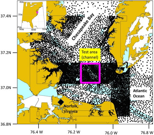
ENC data are provided at a scale appropriate for use, which affects the sounding density. Bands 3, 4, and 5 (“US3x,” “US4x,” and “US5x” here) are, respectively, “Coastal” (lowest density), “Approach,” and “Harbor” (highest density) charts. To simulate the effects of having data in just one of these categories, data from all source charts were exported for “Coastal” (Band 3), “Approach” (Bands 3 and 4), and “Harbor” (Bands 3, 4, and 5) use in the same area (Figure 4). Candidate test areas along both the eastern portion of the dense polygon and the northern portion were considered; the northern portion within the Chesapeake Bay was chosen as it contains a dredged shipping channel that provides diversity in the sounding depths for numerical experiments.

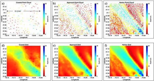
Figure 4. Sounding for the (a) Coastal chart, (b) Approach chart, and (c) Harbor Chart. Panels (d–f) are the gridded bathymetry for these cases, respectively.

Numerical implementations

The point cloud data require processing to the common grid for bathymetry and (subsequent) navigable surfaces. The gridding is a two-step process, as outlined in Appendix C. Implementation was done in MATLAB (Mathworks 2021). Algorithm 1 first augments the xyz point-clouds with additional nodes for stability in subsequent gridding processes in Algorithm 2. Specifically, Algorithm 1 augments the source point cloud data by using (a) Delaunay triangulation routines (Preparata and Shamos 1988) as implemented by MATLAB software and (b) linear interpolation within each triangle to increase the number of points in each irregularly spaced dataset.

Algorithm 2 then (a) grids bathymetry for each of the three datasets, (b) fuses these charts into the shallow and deeper fused surfaces using the OWA for the specific value of $\theta \in \left[0, \left.1\right)\right.$ of interest for the later surface, and (c) computes the navigation category in accord with the process flow given in Section “Overall” process flow. Note from Figure 3 that for edge and corner points, data still exists outside of the boundary. This process is repeated for each chart so that each xyz point-cloud set has a corresponding gridded bathymetry surface. Figures 4d–f show the gridded surfaces of the Figures 4a–c, respectively, for K = 1.

The OWA is then used to obtain the shallow and deep surfaces from these gridded bathymetry surfaces. The shallow reference surface is created by computing the grid for $\theta =0.99.$ Deep bathymetry surfaces are then computed for each of differing values of $\theta$ in the numerical experiments. Soundings used to grid each grid point of the charts are retrieved to compute the navigation category at each grid point. To account for the subjective reliabilities in the Bayesian classifier, the set of reliabilities are divided by the smallest nonzero reliability and then rounded to the nearest integer. This set of integers provides the number of repetitions each irregularly spaced point used in Eq. (10)(10) $${\mu }_i=\frac{\sum _{j=1}^J{R_{j}n}_{i,j}+\sum _{j=1}^J{R_j\alpha }_{i,j}}{\sum _{i=1}^I\sum _{j=1}^J{R_{j}n}_{i,j}+\mathrm{ }{\sum }_i\sum _{j=1}^J{R_j\alpha }_{i,\mathrm{j}}}=\frac{\sum _{j=1}^J{R_{j}n}_{i,j}+{\alpha }_{i,0}}{\sum _{i=1}^I\sum _{j=1}^J{R_{j}n}_{i,j}+\mathrm{ }{\sum }_i{\alpha }_{i,0}}$$(10) to provide the final posterior distribution for that point. Grids for both bathymetry and navigation classes are output from the algorithm.

Results

Figures 4a–c shows the irregularly spaced point cloud data from the ENCs as discussed in Section “Case study area”. For the gridded surfaces, the nearest neighbor in each 45-degree bin was used (i.e. K = 1), so that eight points were used in total for computing each grid point using inverse distance weighting. The corresponding gridded bathymetry surfaces are mapped below each point cloud set in Figures 4d–f. The unnormalized reliabilities for grids corresponding to the Coastal, Approach, and Harbor were subjectively set to $R=\left\{1, 5, 10\right\},$ respectively, based on the qualitative density of points between the datasets. 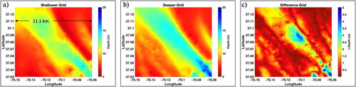Hence, the normalized reliabilities were $r=\left\{1/16, 5/16, 10/16\right\}.$ Figures 5a and b show the shallow and deep surfaces bathymetry surfaces for the case of $\theta =0.1.$ Figure 5c shows the gridded difference between these two surfaces.

Figure 5. Panels (a, b) are aggregated bathymetry grids for the (a) shallow bathymetry surface formed by setting $\theta =0.99$ in the OWA process and (b) deeper bathymetry surface corresponding to $\theta =0.1$ Panel (c) maps the difference between these bathymetry grids.

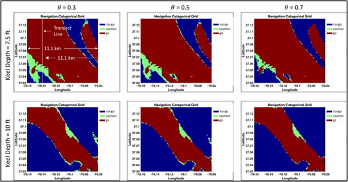
In Figures 6 through 10, two keel depth cases will be discussed: 2.3 m (7.5 feet) and 3.05 m (10 feet). Due to the depth ranges that are present, these cases enable visualization of different effects on the navigation surface with respect to reliability weightings, number of points used for the inverse distance weighted averaging process, keel depth, and attitudinal character.

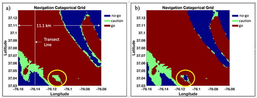
Figures 6a and b shows the navigable surfaces for $\theta =0.1$ resulting for (a) $R=\left\{1, 1, 1\right\},$ i.e. each surface is equally weighted (so that $r=\left\{1/3, 1/3, 1/3\right\}$), and (b) for $R=\left\{1, 5, 10\right\}$ (so that $\mathrm{ }r=\left\{1/16, 5/16, 10/16\right\}).$ The yellow circle indicates a shoal feature that is lost by the equally weighted case. This shoal surface is retained in Figure 6b by using higher reliabilities for denser datasets.

Figure 6. Navigation surface using the OWA for unnormalized reliability weightings of (a) $R=\left\{1, 1, 1\right\}$ and (b) $R=\left\{1, 5, 10\right\}$ as discussed in the text. Source: Author.

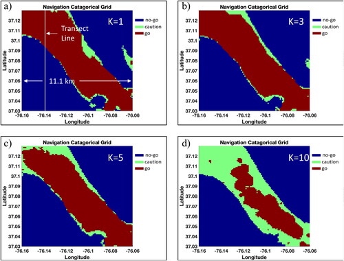
Continuing to use $\theta =0.1$ and $R=\left\{1, 5, 10\right\},$ the results of using K = {1, 3, 5, 10} are illustrated in Figures 7a–d for a 2.3 m (7.5 foot) keel depth. The shoal area in the southeastern portion of the channel no longer maintains the “no-go” category as more nearest neighbors are counted for the navigation category. Using more points leads to smoothing away of the “caution” category for one of the cases. Figures 8a–d show these same results for the 3.05 m (10 foot) keel depth. The shoal area exhibits the same patterns as the 2.3 m keel case. In the northwest and southeast corners, shallower points that are retained in the irregularly scattered data have an effect on changing the “go” category to “caution.”

Figure 7. Navigation surface as nearest neighbors used vary from (a) K = 1, (b) K = 3, (c) K = 5, and (d) K = 10 for the 7.5-foot keel clearance case, $\theta =0.1$ and $R=\left\{1, 5, 10\right\}.$ Source: Author.

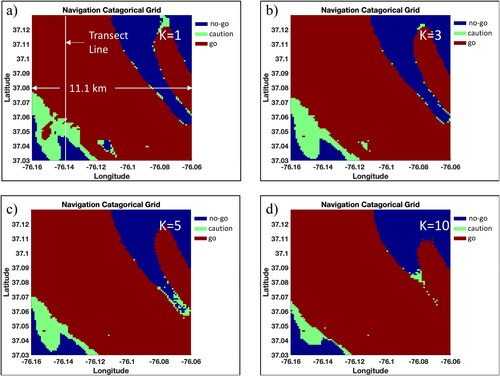
Figure 8. Same as Figure 7, but for the 10-foot keel clearance case. Source: Author.

Retaining K = 1, Figure 9 shows the navigation categories for $\theta =\left\{0.3, 0.5, 0.7\right\}$ for the two keel depths of interest. As is observable, the categories change from “caution” to “no-go” with increasing $\theta$ for the keel depth of 2.3 m. For the 3.05 m depth, these effects are not as drastic. The shoal at (37.04 N, −76.09E) becomes a “no-go” area, along with more of areas on either side of the channel.

Figure 9. Navigation surface for $\theta =\left\{0.3, 0.5, 0.7\right\}$ for the 7.5-foot keel clearance case in subfigures a–c, respectively, and for the 10-foot keel clearance case in subfigures d–f. Source: Author.

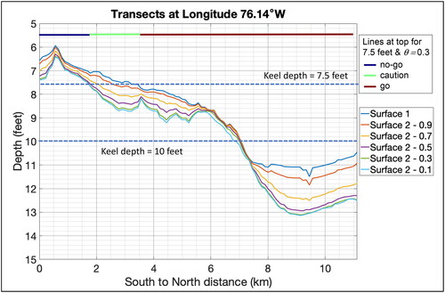
Figure 10 shows the bathymetry along the transect line along −76.14E illustrated in the gridded surfaces for K = 1 and $R=\left\{1, 5, 10\right\}.$ Figure 10 also shows the keel depths of 2.3 m and 3.05 m and the corresponding navigation categories for the 2.3 m keel depth (the navigation category changes for the 3.05 m keel depth simply change from “no-go” to “go” after crossing 37.09 N from the south to the north). Consistent with the graphs in Appendix A and in Figures 8 and 9, Figure 10 plots the 2D effect of adjusting the deep surface for $\theta =\left\{0.1, 0.3, 0.5, 0.7,0.9\right\}.$ This transect shows that higher values of the attitudinal character leads to a shallowing for the deeper surface. We also inspected the difference surfaces as displayed in Figure 5c for higher values of the attitudinal character; the maximum of the difference between shallow and deep surfaces (given by the upper range of the colorbar) decreased with increasing $\theta .$

Figure 10. Transect lines for the vertical line shown in the previous figures for $\theta =\left\{0.1, 0.3, 0.5, 0.7, 0.9\right\}.$

Discussion

The key point in creating the navigable surface is that using lower values of $\theta$ for the deep bathymetry surface results in more “go” categories becoming “caution” categories along the edges of the channel. The deeper that surface is to the reference surface, the more the navigator is hedging for higher safety by putting more of the “go” categories into “caution.” The trade off, it seems, may be false alarms of “caution.” This classification trend of the shoal area in the southern portion of the scene does not occur here until the attitudinal character gets closer to one. This trend indicates that human inspection still is required at this location; such false alarms of “caution” could make the transit longer or impossible (e.g. closed channels) if accepted without inspection.

The concept of optimistic and pessimistic reconstructions in each area directly leads to a model of uncertainty for safety. It is clear that in the region shoalward of the deeper reconstruction, it will be unsafe to travel. In the region deepward of the reconstruction, it will be safe to travel. In between these regions there is a “caution” area. The size of the “caution” area reflects the attitudinal character of risk acceptance in the construction of the navigation surface.

Different categories could be developed that involve the use of linguistic quantifiers for a judgment on the reliability/trust of the information used for assigning R values. These quantifiers could be standardized into a defined set of linguistic terms or identifiers (i.e. terms placed in a look-up table, e.g.). Examples are type identifications used by GEBCO for the GEBCO grid (International Hydrographic Organization 2019) as mentioned in Section “Order weighted averaging” or CATZOCs. The terms then would be translated into R values that are then used by the weight generating function and Bayesian categorical estimator.

The derivation of relative reliability estimates and attitudinal character are subjective, and may develop over time, or through the current tactical situation. By their nature, it is reasonable to assume that reliability estimates will be more stable between observers, however. For example, it seems that a most observers would agree that more dense sources and more recent surveys are likely to be more reliable. Thus within the algorithm, R values would reflect the change of horizontal precision due to cartographic generalization, with higher R values assigned to ENCs with large scale (e.g. Harbor charts should have higher R than Coastal charts) or with more recent survey information.

It also is likely that reliabilities will need to vary spatially, rather than have a single fixed set of values as used here for simplicity, primarily to take into account the large variability in quality in some of the existing ENCs (as depicted by the presence of ENC areas with different CATZOC). Such values might therefore be recommended by a hydrographic agency, or through international agreement and change rarely; recommended values associated with charted data by the hydrographic office might eventually be possible as an adjunct, or alternative, to CATZOC or other data quality measures (Calder et al. 2020).

The attitudinal character, however, is likely to be much more variable since it depends strongly on the navigator’s attitude to risk, which is likely to be affected by a large number of own-ship factors. For example, higher risk might be acceptable for a bulk carrier than a liquified natural gas (LNG) tanker (Calder 2015), although the total cost of an incident might be higher for a large crude oil tanker than for an LNG ship (i.e. the clean-up for an oil incident is significantly higher than for natural gas). Methods developed to elicit level of risk acceptance in operational research (Raiffa and Schlaifer 2000) might be used to assess appropriate values based on ideas of risk, total cost, and utility.

The Concept of Operations (CONOP) for the proposed model is primarily in the planning stages of a ship transit where the goal is to have a more reproduceable (and less mentally taxing) method to fuse a common navigational picture from all of the available data sources. The expectation is that this would most likely take place through a specialized tool attached to the Electronic Chart System (ECS) or Electronic Chart Display and Information System (ECDIS), since they provide the only generally available “point of use” source data for the mariner. (The ECS route is more likely due to International Maritime Organization carriage requirements for ECDIS systems.) The goal would be to allow the navigator to specify reliabilities and attitudinal character, and to vary the assumptions for the planned transit to assess the most plausible route.

The output would most likely be an overlay of the fused categorical classes to be viewed in conjunction with other ENC information; an IHO S-100 series (International Hydrographic Organization 2022) special-purpose cartographic product would be the most likely current implementation model. Use of the S-100 framework for the output has the added benefit of using such standards on the input side as well as it would facilitate the standardized ingestion of other types of information (e.g. S-102 - high resolution bathymetry, S-104 - tidal information). Implementations will likely require software engineering, starting with a relatively simple implementation that relates the algorithm parameters to existing ENC quality indicators, such as CATZOC and date of the latest applied updates. Such implementations could then be made available for end-user software, such as a plugin for open-source OpenCPN (2022) in the Safety plugins category.

Some research questions involving human factors remain open and include the question of what visualization model would work best for this data. For planning, a simple “traffic light” scheme of red (no-go), yellow (caution), and green (go) transparent coloring might be sufficient, but overlays of this kind are known to obscure detail, making them hard to use in practice. Current research (Kastrisios and Ware 2022) on display of uncertainty data for bathymetry in a navigational context might be used to provide better approaches. Another open question with regard to CONOPs is whether the proposed method is better for planning, or if they can be used during operations (e.g. to provide decision support if the ship has to deviate from the planned route). The requirements for real-time support are quite different from planning, and further research would likely be required to determine the best method to provide this information, and effective visualization techniques that provide support without clutter on the display.

Further work also could include the use of available types of S57 hazards that make the reconstruction more adherent to the human interpretation of a real ENC; the paper by Masetti, Faulkes, and Kastrisios (2018) can serve as a starting point. Some of these objects, for instance wrecks (WRECKS) and obstructions (OBSTRN), will require a slightly more sophisticated treatment that the simple extraction of the value of sounding (VALSOU, if available) as they could necessitate the creation of a buffer area around the feature position to reflect horizontal uncertainty of the report. One could translate linguistic terms for hazards into automatic “no-go” regions that would then override the Bayesian output for that position through possibilistic conditioning (Yager 2012; Elmore, Petry, and Yager 2014) or possibility-probability transformations (Petry, Elmore, and Yager 2015).

Additional work also could include temporal dependency built into the algorithm that makes grid nodes become more pessimistic based on age of the information. In addition, analysis of the shape of the estimated categorical distribution (e.g. through the kurtosis, measuring the “peaked-ness” of the distribution) at each location can be used to determine the degree of consistency of the various sources, which could also be displayed to the user as qualifying information for the algorithm and data. Further, other algorithms for performing the irregular interpolation of the bathymetry soundings other than the average of enclosing TIN points could be implemented, such as those based on B-Splines (Steinbeck and Koschke 2021). In addition, the algorithms and framework developed in this article could further be used in a secondary fusion process of navigation risk surfaces and safety contours as emerging navigation risk tools (Bakdi et al. 2019; Jeong et al. 2019) become available.

Summary

This article provides a hybrid-framework for human-in-the-loop information fusion of navigation planning. Because the human-in-the-loop is core to this problem, a soft computing methodology (OWA) designed for such information fusion is used along with Bayesian estimates of risk categories. The framework shows how to compute OWA weights when human judgment of reliability of the information sources is involved, along with attitudinal character of risk tolerance. The estimates of reliability are reused in the Bayesian process of computing the categorical risk by providing the number of extra counts used in the Dirichlet-based maximum likelihood estimation of the probability for each category. The final category assigned is the category with the highest posterior probability, with ties broken toward the most pessimistic category.

Simple examples of using this method to compute an average of bathymetry were presented. This process forms the basis of the overall computational flow used in the case study. In the case study, maps that show areas for safe, cautionary, or unsafe navigation (“go,” “caution,” and “no-go” areas) are presented for an area of the Chesapeake Bay. Differing maps are constructed with differing sounding densities from ENC data. The framework takes irregularly spaced sounding data and computes a common gridded bathymetry surface for each chart set. Demonstrations of navigation risk surfaces computed through the OWA and Bayesian fusion are shown for differing levels of attitudinal character of risk tolerance. As the attitudinal character is lowered (tending to a more conservative approach), more area of navigation surface that were “go” change to “caution” areas along classification boundaries. This change reflects the navigator’s desire for extra keel clearance. The case study also shows how keel depth, risk tolerance, judgment of data reliability, and spatial extent of information used (by number of nearest neighbors) can affect the risk surface calculation by averaging away hazardous areas.

This framework provides a means of being able to record judgments made of data reliability. This recoding capability enables reproducibility of the resultant human-based map of navigation risk. This framework can be further be used for subsequent fusion of differing assessments of navigation risk as future capabilities and software of estimating navigation risk and safety are developed and emerge for use.

Acknowledgments

The main authors wish to thank R. Wade Ladner, Raymond Sawyer, and Dr. David Fabre of the Naval Oceanographic Office and Brett Hode of the Naval Research Laboratory for their helpful discussions in the initial phase of research. The authors wish to thank all of the funding sources for their sponsorship of this research and the anonymous peer-reviewers for their guidance in revising this manuscript.

Disclosure statement

No potential conflict of interest was reported by the authors.

Data availability statement

The data that support the findings of this study are openly available at https://nauticalcharts.noaa.gov/charts/noaa-enc.html.

Additional information

Funding

Initial funding for the conceptual development of this work was provided by the Office of Naval Research10.13039/100000006. Additional funding for generation of this paper was given to Elmore through a Janney grant of the Johns Hopkins University/Applied Physics Laboratory10.13039/100012314 and to Petry through the Naval Research Laboratory’s Base Program. Funding for Calder and Massetti was also provided by NOAA10.13039/100000192 grant NA20NOS4000196.

Appendix A

Figure associated with examples

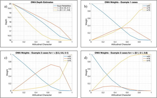
Figure A1 below provides graphs of the depth estimates and OWA weights as a function of attitudinal character for the cases discussed in the body of this article.

Figure A1. Graphs corresponding to the examples given in this Appendix showing depth estimates and weightings as a function of attitudinal character. Subfigure (a): depth estimates for equal reliability weighting in blue, $r=\{0.3, 0.6, 0.1\}$ in red, and $r=\{0.1, 0.1, 0.8\}$ in yellow. Subfigures (b–d): OWA weights for the three data points (z = 20 feet in blue, z = 18 feet in red, and z = 16 feet in yellow) with attitudinal character for (b) the equal reliability case, (c) the $r=\{0.3, 0.6, 0.1\}$ case, and (d) the $r=\{0.3, 0.6, 0.1\}$ case.

Appendix B

Derivation of weighted Dirichlet expectation values

This appendix derives Eqs. $(9)$ and $(10).$ Equation $(9)$ is expectation value for the ith category which is derived in Appendix Section B (Derivation of Eq. $(9)$). Section Derivation of Eq. (10)(10) $${\mu }_i=\frac{\sum _{j=1}^J{R_{j}n}_{i,j}+\sum _{j=1}^J{R_j\alpha }_{i,j}}{\sum _{i=1}^I\sum _{j=1}^J{R_{j}n}_{i,j}+\mathrm{ }{\sum }_i\sum _{j=1}^J{R_j\alpha }_{i,\mathrm{j}}}=\frac{\sum _{j=1}^J{R_{j}n}_{i,j}+{\alpha }_{i,0}}{\sum _{i=1}^I\sum _{j=1}^J{R_{j}n}_{i,j}+\mathrm{ }{\sum }_i{\alpha }_{i,0}}$$(10) will make use of the result of Section B (Derivation of Eq. (9)) to derive Eq. $(10).$ The goal of these derivations is to show that weighting the jth dataset by $R_j$ (where $R_j\in {\mathbb{Z}}^{+}$) is equivalent to recounting the dataset $R_j$ times for our use of Dirichlet categorical estimation.

Derivation of Eq. $(9)$

This section follows derivation methods from the YouTube series by Mathematicalmonk (2012). The derivation below has three major components: (1) initial setup of the problem in the context of counting categories, (2) providing useful substitutions and relations, and (3) use of substitutions to complete the derivation. The gamma function, $\mathrm{\Gamma }\left(n\right)$ is core to the Dirichlet probability density function. In the present problem, $n$ is an integer, which means that (B1) $$\mathrm{\Gamma }\left(n\right)=\left(n-1\right)!;\mathrm{ }n\in \mathbb{Z}$$(B1)

The expectation is derived explicitly for the category with $i=1,$ but extension to categories with $i\ne 1$ is obvious.

Initial setup

Let ${\alpha }_{\mathrm{\Sigma }}\equiv {\sum }_{i=1}^{i=I}{\alpha }_i$ where ${\alpha }_i$ is the number of counts for the ith category, with an initial value for each being ${\alpha }_{i,0}>0 \forall i.$ For categories $i=1, 2,\dots ,I,$ the Dirichlet probability density function is (B2) $$p\left({\theta }_1,\mathrm{ }\dots ,{\theta }_I;\mathrm{ }{\alpha }_1,\dots ,{\alpha }_I\right)=\frac{\mathrm{\Gamma }\left({\alpha }_{\mathrm{\Sigma }}\right)}{\mathrm{\Gamma }\left({\alpha }_1\right)\mathrm{\Gamma }\left({\alpha }_2\right)\times \cdots \times \mathrm{\Gamma }\left({\alpha }_I\right)}\prod _{i=1}^I{\theta }_i^{{\alpha }_i-1}$$(B2) where ${\sum }_{i=1}^{i=I}{\theta }_i=1,$ with each ${\theta }_i$ representing the probability mass for the ith category. The expectation value for parameter ${\theta }_1$ is (B3) $${\mu }_1\equiv E\left({\theta }_1\right)=\int {\theta }_1\frac{\mathrm{\Gamma }\left({\alpha }_{\mathrm{\Sigma }}\right)}{\mathrm{\Gamma }\left({\alpha }_1\right)\mathrm{\Gamma }\left({\alpha }_2\right)\times \cdots \times \mathrm{\Gamma }\left({\alpha }_I\right)}\prod _{i=1}^I{\theta }_i^{{\alpha }_i-1}d\theta$$(B3)

Notice that ${\theta }_1{\prod }_{i=1}^I{\theta }_i^{{\alpha }_i-1}={\theta }_1{\theta }_1^{{\alpha }_1-1}{\prod }_{i=2}^I{\theta }_i^{{\alpha }_i-1}={\theta }_1^{{\alpha }_1}{\prod }_{i=2}^I{\theta }_i^{{\alpha }_i-1}.$ Thus, Eq. (B3)(B3) $${\mu }_1\equiv E\left({\theta }_1\right)=\int {\theta }_1\frac{\mathrm{\Gamma }\left({\alpha }_{\mathrm{\Sigma }}\right)}{\mathrm{\Gamma }\left({\alpha }_1\right)\mathrm{\Gamma }\left({\alpha }_2\right)\times \cdots \times \mathrm{\Gamma }\left({\alpha }_I\right)}\prod _{i=1}^I{\theta }_i^{{\alpha }_i-1}d\theta$$(B3) becomes (B4) $${\mu }_1\equiv E\left({\theta }_1\right)=\int \frac{\mathrm{\Gamma }\left({\alpha }_{\mathrm{\Sigma }}\right)}{\mathrm{\Gamma }\left({\alpha }_1\right)\mathrm{\Gamma }\left({\alpha }_2\right)\times \cdots \times \mathrm{\Gamma }\left({\alpha }_I\right)}{\theta }_1^{{\alpha }_1}\prod _{i=2}^I{\theta }_i^{{\alpha }_i-1}d\theta$$(B4)

Useful substitutions and relations

A useful recursion relation of the gamma function that this derivation will exploit is (B5) $$\mathrm{\Gamma }\left(n+1\right)=n\mathrm{\Gamma }\left(n\right)$$(B5)

Define, ${\beta }_1\equiv {\alpha }_1+1,$ ${\beta }_i\equiv {\alpha }_i\mathrm{ }\text{for}\mathrm{ }i\ge 2,$ and ${\beta }_{\mathrm{\Sigma }}\equiv {\sum }_{i=1}^{i=I}{\beta }_i.$ Note that ${\beta }_{\mathrm{\Sigma }}={\alpha }_{\mathrm{\Sigma }}+1.$ Thus, with Eq. ($\mathrm{B}$5), the following useful relations hold (B6) $$\mathrm{\Gamma }\left({\alpha }_1+1\right)={\alpha }_1\mathrm{\Gamma }\left({\alpha }_1\right)$$(B6) (B7) $$\mathrm{\Gamma }\left({\alpha }_{\mathrm{\Sigma }}+1\right)={\alpha }_{\mathrm{\Sigma }}\mathrm{\Gamma }\left({\alpha }_{\mathrm{\Sigma }}\right)$$(B7) (B8) $$\mathrm{\Gamma }\left({\beta }_1\right)=\mathrm{\Gamma }\left({\alpha }_1+1\right)={\alpha }_1\mathrm{\Gamma }\left({\alpha }_1\right)$$(B8) (B9) $$\mathrm{\Gamma }\left({\beta }_{\mathrm{\Sigma }}\right)=\mathrm{\Gamma }\left({\alpha }_{\mathrm{\Sigma }}+1\right)={\alpha }_{\mathrm{\Sigma }}\mathrm{\Gamma }\left({\alpha }_{\mathrm{\Sigma }}\right)$$(B9) (B10) $$\mathrm{\Gamma }\left({\alpha }_1\right)=\mathrm{\Gamma }\left({\beta }_1\right)/{\alpha }_1$$(B10) (B11) $$\mathrm{\Gamma }\left({\alpha }_{\mathrm{\Sigma }}\right)=\mathrm{\Gamma }\left({\beta }_{\mathrm{\Sigma }}\right)/{\alpha }_{\mathrm{\Sigma }}$$(B11)

Completion of the derivation

Using Eqs. (B10)(B10) $$\mathrm{\Gamma }\left({\alpha }_1\right)=\mathrm{\Gamma }\left({\beta }_1\right)/{\alpha }_1$$(B10) and (B11)(B11) $$\mathrm{\Gamma }\left({\alpha }_{\mathrm{\Sigma }}\right)=\mathrm{\Gamma }\left({\beta }_{\mathrm{\Sigma }}\right)/{\alpha }_{\mathrm{\Sigma }}$$(B11) in Eq. (B4)(B4) $${\mu }_1\equiv E\left({\theta }_1\right)=\int \frac{\mathrm{\Gamma }\left({\alpha }_{\mathrm{\Sigma }}\right)}{\mathrm{\Gamma }\left({\alpha }_1\right)\mathrm{\Gamma }\left({\alpha }_2\right)\times \cdots \times \mathrm{\Gamma }\left({\alpha }_I\right)}{\theta }_1^{{\alpha }_1}\prod _{i=2}^I{\theta }_i^{{\alpha }_i-1}d\theta$$(B4) yields (B12) $${\mu }_1\equiv E\left({\theta }_1\right)=\int \frac{{\alpha }_1}{{\alpha }_{\mathrm{\Sigma }}}\frac{\mathrm{\Gamma }\left({\beta }_{\mathrm{\Sigma }}\right){\theta }_1^{{\alpha }_1}}{\mathrm{\Gamma }\left({\beta }_1\right)\mathrm{\Gamma }\left({\beta }_2\right)\times \cdots \times \mathrm{\Gamma }\left({\beta }_I\right)}\prod _{i=2}^I{\theta }_i^{{\beta }_i-1}d\theta$$(B12)

Note that ${\alpha }_1={(\alpha }_1+1)-1={\beta }_1-1$ so that (B13) $${\mu }_1\equiv E\left({\theta }_1\right)=\int \frac{{\alpha }_1}{{\alpha }_{\mathrm{\Sigma }}}\frac{\mathrm{\Gamma }\left({\beta }_{\mathrm{\Sigma }}\right){\theta }_1^{{(\alpha }_1+1)-1}}{\mathrm{\Gamma }\left({\beta }_1\right)\mathrm{\Gamma }\left({\beta }_2\right)\times \cdots \times \mathrm{\Gamma }\left({\beta }_I\right)}\prod _{i=2}^I{\theta }_i^{{\beta }_i-1}d\theta$$(B13) (B14) $$=\int \frac{{\alpha }_1}{{\alpha }_{\mathrm{\Sigma }}}\frac{\mathrm{\Gamma }\left({\beta }_{\mathrm{\Sigma }}\right){\theta }_1^{{\beta }_1-1}}{\mathrm{\Gamma }\left({\beta }_1\right)\mathrm{\Gamma }\left({\beta }_2\right)\times \cdots \times \mathrm{\Gamma }\left({\beta }_I\right)}\prod _{i=2}^I{\theta }_i^{{\beta }_i-1}d\theta$$(B14) (B15) $$=\frac{{\alpha }_1}{{\alpha }_{\mathrm{\Sigma }}}\int \frac{\mathrm{\Gamma }\left({\beta }_{\mathrm{\Sigma }}\right)}{\mathrm{\Gamma }\left({\beta }_1\right)\mathrm{\Gamma }\left({\beta }_2\right)\times \cdots \times \mathrm{\Gamma }\left({\beta }_I\right)}\prod _{i=1}^I{\theta }_i^{{\beta }_i-1}d\theta$$(B15)

The function in the integral is a Dirichlet probability density function, which must integrate to 1. Thus, (B16) $${\mu }_1\equiv E\left({\theta }_1\right)=\frac{{\alpha }_1}{{\alpha }_{\mathrm{\Sigma }}}$$(B16)

Now, set ${\alpha }_{i,0}=1 \forall i$ for the initial prior pdf, and $n_i={\alpha }_i$ after counting of the ith category is complete and $N={\sum }_i{n}_i.$ Thus ${\alpha }_1=n_i+{\alpha }_{i,0}$ and ${\alpha }_{\mathrm{\Sigma }}=N+{\sum }_i{\alpha }_{i,0}.$ These substitution in (B16) yields Eq. $(9).$

Derivation of Eq. $(10)$

From Eq. (B11)(B11) $$\mathrm{\Gamma }\left({\alpha }_{\mathrm{\Sigma }}\right)=\mathrm{\Gamma }\left({\beta }_{\mathrm{\Sigma }}\right)/{\alpha }_{\mathrm{\Sigma }}$$(B11) , let $n_i={\sum }_{j=1}^J{n}_{i,j}$ where $j=1, 2,\dots ,J$ indexes the dataset used. Then, $N={\sum }_{i=1}^I{\sum }_{j=1}^J{n}_{i,j}$ and $a_{i,0}={\sum }_{j=1}^J{\alpha }_{ij,0}.$ (For now, the initial setting for ${\alpha }_{ij,0}$ is abstract, but will set later in this derivation.) With these substitution, Eq. (B11)(B11) $$\mathrm{\Gamma }\left({\alpha }_{\mathrm{\Sigma }}\right)=\mathrm{\Gamma }\left({\beta }_{\mathrm{\Sigma }}\right)/{\alpha }_{\mathrm{\Sigma }}$$(B11) becomes (B17) $${\mu }_i=\frac{n_i+{\alpha }_{i,0}}{N+\mathrm{ }{\sum }_i{\alpha }_{i,0}}=\frac{{\sum }_{j=1}^J{n}_{i,j}+{\sum }_{j=1}^J{\alpha }_{ij,0}}{{\sum }_{i=1}^I{\sum }_{j=1}^J{n}_{i,k}+\mathrm{ }{\sum }_{i=1}^I{\sum }_{j=1}^J{\alpha }_{ij,0}}$$(B17)

If the data are now weighted by normalized reliability $r_k$ (i.e. ${\sum }_{j=1}^J{r}_j=1),$ then, Eq. (B17)(B17) $${\mu }_i=\frac{n_i+{\alpha }_{i,0}}{N+\mathrm{ }{\sum }_i{\alpha }_{i,0}}=\frac{{\sum }_{j=1}^J{n}_{i,j}+{\sum }_{j=1}^J{\alpha }_{ij,0}}{{\sum }_{i=1}^I{\sum }_{j=1}^J{n}_{i,k}+\mathrm{ }{\sum }_{i=1}^I{\sum }_{j=1}^J{\alpha }_{ij,0}}$$(B17) becomes (B18) $${\mu }_i=\frac{{\sum }_{j=1}^J{r}_j{n}_{i,j}+{\sum }_{j=1}^J{r_j\alpha }_{ij,0}}{{\sum }_{i=1}^I{\sum }_{j=1}^J{r_{j}n}_{i,j}+\mathrm{ }{\sum }_{i=1}^I{\sum }_{j=1}^J{r_j\alpha }_{ij,0}}$$(B18)

This result follows from the derivation in Section B (Derivation of Eq. $(9)$) with substitution of ${\alpha }_i$ = ${\sum }_{j=1}^J{r}_j{\alpha }_{i,j}$ and softening the restriction that the gamma function has an integer argument.

As discussed in the main text of the article, $r_j\equiv R_j/{\sum }_{j=1}^J{R}_j,$ where $R_j\in {\mathbb{Z}}^{+}.$ Thus, Eq. (B18)(B18) $${\mu }_i=\frac{{\sum }_{j=1}^J{r}_j{n}_{i,j}+{\sum }_{j=1}^J{r_j\alpha }_{ij,0}}{{\sum }_{i=1}^I{\sum }_{j=1}^J{r_{j}n}_{i,j}+\mathrm{ }{\sum }_{i=1}^I{\sum }_{j=1}^J{r_j\alpha }_{ij,0}}$$(B18) becomes (B19) $${\mu }_i=\frac{{\sum }_{j=1}^J\left(R_j/{\sum }_{j=1}^J{R}_j\right)n_{i,j}+{\sum }_{j=1}^J{\left(R_j/{\sum }_{j=1}^J{R}_j\right)\alpha }_{ij,0}}{{\sum }_{i=1}^I{\sum }_{j=1}^J{\left(R_j/{\sum }_{j=1}^J{R}_j\right)n}_{i,j}+\mathrm{ }{\sum }_{i=1}^I{\sum }_{j=1}^J{\left(R_j/{\sum }_{j=1}^J{R}_j\right)\alpha }_{ij,0}}$$(B19) (B20) $$=\frac{{\sum }_{j=1}^J{R}_j{n}_{i,j}+{\sum }_{j=1}^J{R_j\alpha }_{ij,0}}{{\sum }_{i=1}^I{\sum }_{j=1}^J{R_{j}n}_{i,j}+\mathrm{ }{\sum }_{i=1}^I{\sum }_{j=1}^J{R_j\alpha }_{ij,0}}$$(B20) since all terms in (B20) are divided by ${\sum }_{j=1}^J{R}_j.$ Setting ${\alpha }_{ij,0}={\alpha }_{i,0}/\left(J{R}_j\right),$ Eq. (B20)(B20) $$=\frac{{\sum }_{j=1}^J{R}_j{n}_{i,j}+{\sum }_{j=1}^J{R_j\alpha }_{ij,0}}{{\sum }_{i=1}^I{\sum }_{j=1}^J{R_{j}n}_{i,j}+\mathrm{ }{\sum }_{i=1}^I{\sum }_{j=1}^J{R_j\alpha }_{ij,0}}$$(B20) becomes Eq. (B12)(B12) $${\mu }_1\equiv E\left({\theta }_1\right)=\int \frac{{\alpha }_1}{{\alpha }_{\mathrm{\Sigma }}}\frac{\mathrm{\Gamma }\left({\beta }_{\mathrm{\Sigma }}\right){\theta }_1^{{\alpha }_1}}{\mathrm{\Gamma }\left({\beta }_1\right)\mathrm{\Gamma }\left({\beta }_2\right)\times \cdots \times \mathrm{\Gamma }\left({\beta }_I\right)}\prod _{i=2}^I{\theta }_i^{{\beta }_i-1}d\theta$$(B12) in the text (i.e. one is informed of how to construct the initial Dirichlet pdf using the reliabilities.) Thus, one can account for reliability weighting of the jth chart by recounting each category $R_j$ times. In the special case of $R_j=1 \forall j,$ Eqs. $(10)$ and (B20) reduces to Eq. $(9)$ as required.

Appendix C

Algorithm sketches

Algorithm 1

• Input Parameters: (a) depth clearance; (b) degree of optimism (from 0 to 1)

• Load chart point cloud

• Perform Delaunay triangulation

• FOR each triangle set bv

  • Evaluate the depth of the end nodes for each created triangle

  • IF the end nodes are within the depth clearance

    • Compute depth in the triangle center from linear interpolation

    • Append new triplet to the point cloud.

  • ELSE - skip to next triangle

• Write augmented XYZ point-cloud to output file.

Algorithm 2

• Input Parameters: (a) XY output grid points; (b) depth clearance; (c) number of points to examine at each node; (d) number used indicate no data

• Load augmented point cloud files from Algorithm 1; retain file name string in memory

• FOR each $\theta \in \left\{{\theta }_{\mathrm{*}},{\theta }^{\mathrm{*}}\right\}$

  • FOR each XY grid point

    • Divide the area around each node into octants

    • For each octant, identify the closest xyz-points from the augmented point-cloud

    • IF xyz-data in at least one octant,

      • XY gridded bathymetry value = average of these nearest xyz-points weighted by the inverse of the squared distance

    • ELSE

      • XY gridded bathymetry value = no data flag (manual intervention will be required to augment the data)

  • WRITE gridded bathymetry to output files for each $\theta \in \left\{{\theta }_{*},{\theta }^{*}\right\}$

• Transform bathymetry to trinary output classes is finally created by using pair of grids (with different degree of optimism) as follows:

• For each cell in the grid pair for $\theta \in \left\{{\theta }_{*},{\theta }^{*}\right\},$ set the quaternary value as follows:

  • 3 (no-go): keel depth is either deeper than the (a) sounding depth OR (b) deeper reference depth

  • 1 (go): keel depth is shallower than the (a) sounding depth AND (b) shallow reference depth

  • 2 (maybe): keel depth is in between the two reference depths AND (b) the sounding is in between the two surfaces

• WRITE trinary output to output file grid

References

- Bakdi, A., I. K. Glad, E. Vanem, and O. Engelhardtsen. 2019. AIS-based multiple vessel collision and grounding risk identification based on adaptive safety domain. Journal of Marine Science and Engineering 8 (1):Article 5.
- Beliakov, G., A. Pradera, and T. Calvo. 2007. Aggregation functions: A guide for practitioners. Heidelberg: Springer. ISBN: 978–3540737209.
- Calder, B. 2015. On risk-based expression of hydrographic uncertainty. Marine Geodesy 38 (2):99–127.
- Calder, B. R., S. J. Dijkstra, S. Hoy, K. Himschoot, and A. Schofield. 2020. A design for a trusted community bathymetry system. Marine Geodesy 43 (4):327–58.
- Chénier, R., M. Sagram, K. Omari, and A. Jirovec. 2020. Earth observation and artificial intelligence for improving safety to navigation in Canada low-impact shipping corridors. ISPRS International Journal of Geo-Information 9 (6):383.
- Cutler, T. 2003. Dutton’s nautical navigation. 15th ed. Annapolis, MD: Naval Institute Press. ISBN 978-1-55750-248-3.
- Elmore, P., F. Petry, and R. Yager. 2014. Comparative measures of aggregated uncertainty representations. Journal of Ambient Intelligence and Humanized Computing 5 (6):809–19.
- EMODnet Bathymetry Consortium. 2020. EMODnet digital bathymetry (DTM). Accessed January 13, 2023. https://doi.org/10.12770/bb6a87dd-e579-4036-abe1-e649cea9881a
- Gelman, A., J. B. Carlin, H. S. Stern, D. B. Dunson, A. Vehtari, and D. B. Rubin. 2013. Bayesian data analysis. 3rd ed. Boca Raton, Florida: Chapman and Hall/CRC. ISBN: 978–1439840955
- Gilardoni, E., and J. Presedo. 2017. Navigation in shallow waters. Livingston Scotland, UK: Witherbys Publishing. ISBN: 978–1856096676.
- International Hydrographic Organization. 2000. Intergovernmental Oceanographic Commission, IHO Transfer Standard for Digital Hydrographic Data, IHO Publication S-57, Edition 3.10. Accessed January 27, 2022. https://iho.int/uploads/user/pubs/standards/s-57/31main.pdf.
- International Hydrographic Organization. 2019. Intergovernmental Oceanographic Commission, The IHO-IOC GEBCO Cook Book, IHO Publication B-11, Monaco, October 2019. Accessed January 27, 2022. https://www.gebco.net/data_and_products/gebco_cook_book/.
- International Hydrographic Organization. 2020. Intergovernmental Oceanographic Commission, Mariner’s Guide to Accuracy of Depth Information in Electronic Navigational Charts (ENC), IHO Publication S-67, Edition 1.0.0. Accessed November 21, 2022. https://iho.int/en/standards-and-specifications.
- International Hydrographic Organization. 2022. Intergovernmental Oceanographic Commission, S-100 Universal Hydrographic Data Model. Accessed November 25, 2022. http://iho.int/en/s-100-universal-hydrographic-data-model.
- Jakobsson, M., L. A. Mayer, C. Bringensparr, C. F. Castro, R. Mohammad, P. Johnson, T. Ketter, D. Accettella, D. Amblas, L. An, et al. 2020. The International Bathymetric Chart of the Arctic Ocean Version 4.0. Scientific Data 7 (1):176.
- Jeong, M. G., E. B. Lee, M. Lee, and J. Y. Jung. 2019. Multi-criteria route planning with risk contour map for smart navigation. Ocean Engineering 172:72–85.
- Kastrisios, C., and C. Ware. 2022. Textures for coding bathymetric data quality sectors on electronic navigational chart displays: Design and evaluation. Cartography and Geographic Information Science 49 (6):492–511.
- Kastrisios, C., C. Ware, B. Calder, T. Butiewicz, L. Alexander, and O. Hauser. 2020. Nautical chart data uncertainty visualization as the means for integrating bathymetric, meteorological, and oceanographic information in support of coastal navigation. Presented at the Proceedings of the American Meteorological Society 100th Meeting. Boston, MA. Accessed January 27, 2022. http://ccom.unh.edu/sites/default/files/publications/Kastrisios_etal_AMS2020_Abstract_ChartDataUncertaintyVisualizationAndIntegration.pdf.
- Masetti, G., T. Faulkes, and C. Kastrisios. 2018. Automated identification of discrepancies between nautical charts and survey soundings. ISPRS International Journal of Geo-Information 7 (10):392.
- Mathematicalmonk. 2012. Expectation of a Dirichlet random variable. Palo Alto, CA: YouTube video hosted by Google. Accessed March 25, 2022. https://youtu.be/emnfq4txDuI.
- Mathworks. 2021. MATLAB (Version 2021b). Natick, MA: The Mathworks Inc. Accessed January 27, 2022. www.mathworks.com.
- Naevestad, T. O., R. O. Phillips, K. V. Størkersen, A. Laiou, and G. Yannis. 2019. Safety culture in maritime transport in Norway and Greece: Exploring national, sectorial and organizational influences on unsafe behaviours and work accidents. Marine Policy 99:1–13.
- National Oceanic and Atmospheric Administration – Office of Coastal Survey. 2022. NOAA ENC – Electronic Navigation Charts. Accessed January 27, 2022. https://nauticalcharts.noaa.gov/charts/noaa-enc.html.
- OpenCPN. 2022. OpenCPN Chart Plotter Navigation, Version 5.6.2. Accessed November 25, 2022. https://www.openCPN.org.
- Petry, F., P. Elmore, and R. Yager. 2015. Combining uncertain information of differing modalities. Information Sciences 322:237–56.
- Preparata, F., and M. Shamos. 1988. Computational geometry - An introduction. Springer-Verlag Berlin: GDR. ISBN: 978–0387961316.
- QGIS.org. 2020. QGIS Geographic Information System, Version 3.12. QGIS Association. Accessed January 13, 2023. http://www.qgis.org.
- Raiffa, H., and R. Schlaifer. 2000. Applied statistical decision theory. New York: Wiley Classics Library. Wiley.
- Saddler, R. 2006. Graveyard of the Pacific: Gateway to the Northwest. Accessed November 24, 2021. https://www.blueoregon.com/2006/01/graveyard_of_th/.
- Steinbeck, M., and R. Koschke. 2021. TinySpline: A small, yet powerful library for interpolating, transforming, and querying NURBS, B-splines, and Bezier curves. Paper presented at the 28th IEEE International Conference on Software Analysis, Evolution and Reengineering (SANER), (Virtual Meeting), Honolulu, HI, March 09–12.
- Walhey, F. 2013. U.S. navy to scrap vessel stuck on Philippine reef. New York Times, January 31. Accessed January 27, 2022. https://www.nytimes.com/2013/02/01/world/asia/us-navy-to-scrap-vessel-stuck-on-philippine-reef.html.
- Weatherall, P., K. M. Marks, M. Jakobsson, T. Schmitt, S. Tani, J. E. Arndt, M. Rovere, D. Chayes, V. Ferrini, R. Wigley, et al. 2015. A new digital bathymetric model of the world’s oceans. Earth and Space Science 2 (8):331–45.
- Wilma, D. 2006. Graveyard of the Pacific: Shipwrecks on the Washington Coast. Accessed November 24, 2021. https://www.historylink.org/File/7936.
- Yager, R. 1988. On ordered weighted averaging aggregation operators in multicriteria decision making. IEEE Transactions on Systems, Man, and Cybernetics 18 (1):183–90.
- Yager, R., P. Elmore, and F. Petry. 2017. Soft likelihood in combining evidence. Information Fusion 36:185–90.
- Yager, R. R. 2012. Conditional approach to possibility-probability fusion. IEEE Transactions on Fuzzy Systems 20 (1):46–56.
- Yager, R. R., and J. Kacprzyk. 1997. The ordered weighted averaging operators: Theory and applications. Norwell, MA: Kluwer. ISBN: 978–0792399346