Low-cost multi-GNSS, single-frequency RTK averaging for marine applications: accurate stationary positioning and vertical tide measurements

Abstract

The use of Real Time Kinematic (RTK) Global Navigation Satellite System (GNSS) for accurate horizontal and vertical measurements in the marine environment has been considered since the late-1980’s and tested from the 1990’s when GPS and GLONASS were the only operational constellations available and high-cost multi-frequency receiver equipment was required. This paper modernizes the conversation using multi-constellation, low-cost, single-frequency RTK GNSS measurements and proves their value with accurate positioning and tide measurements. Our tests show average stationary horizontal positioning measurements using this equipment are suitable (95% CI) for the most stringent International Hydrographic Organization (IHO) Standard S-44 ‘Exclusive Order’ at base station ranges of up to 27 km. Vertical observations on a moving platform, smoothed using a baseline distance-dependent moving average filter show the equipment and method are comparable with traditional electronic tide gauge observations over the same base station range. All of our measurement results show the potential to improve total uncertainty calculations undertaken by hydrographers, engineers and scientists in the marine realm, while the low-cost equipment raises the possibility that more measurements can be taken, leading to improvements in monitoring, modelling and understanding the marine environment.

Keywords:

• Low-cost GNSS
• real-time kinematic positioning (RTK)
• single-frequency GNSS
• RTK tides
• hydrography
• International Hydrographic Organization (IHO) Order

Introduction

The Real Time Kinematic (RTK) Global Navigation Satellite System (GNSS) positioning model combines observations from two receivers with integer ambiguity resolution to reduce the relative effects of the ionosphere and troposphere on the GNSS measurement (Langley, Teunissen, and Montenbruck 2017). With one receiver acting as a base station at a known location, corrections can be sent to the other receiver operating in a kinematic mode. If the separation between the two receivers is kept within a few tens of kilometers, it is generally possible to derive real-time, or near-real-time, centimeter level positions at the kinematic station (Odijk 2017). In the past this method has required equipment that can track satellites on dual-frequencies: e.g. Global Positioning System (GPS) L1 and L2 bands. Survey-grade receivers capable of this multi-frequency tracking can cost up to several thousand, or tens of thousands, of dollars (Odolinski and Teunissen 2016).

The advent of constellations such as the Russian Global Navigation Satellite System (GLONASS), Chinese BeiDou (BDS), European Galileo and Japanese Quasi-Zenith Satellite System (QZSS), when combined with the established United States (US) American GPS, provide a growing number of satellites available for observation and improved methodologies (Naismith, Jeffress, and Prouty 1999, Thom et al. 2019). The addition of QZSS observations to GPS/Galileo/BDS derived positions by Odolinski, Teunissen, and Odijk (2015) showed that one could use an elevation cut-off angle of 30 degrees and still obtain 100% availability of positioning precisions at the mm-level in a single-epoch RTK mode.

With the increase in available constellations comes redundancy and the ability to achieve accurate RTK measurements with much lower-cost single-frequency GNSS equipment (Odolinski and Teunissen 2019, 2016). By lowering the cost of RTK GNSS equipment to only a few hundreds of dollars (USD, with costs decreasing as time goes on), wide-ranging improvements can be made in fields that require accurate real-time positioning, such as construction engineering, hydrography, cadastral surveying, precision agriculture, autonomous vehicle use and aircraft navigation (e.g. He 2010, Dabove 2019, Tradacete et al. 2019).

The use of high-accuracy, high-precision, centimeter-level measurements improves all aspects of 3D positioning. Many of the benefits of using RTK GNSS in the marine environment by hydrographers, marine engineers and scientists are well known (FIG Commission 4 2010, Mills and Dodd 2014, Ligteringen, Loog, and Dorst 2014, DeLoach 1995, Wells and Kleusberg 1992). In hydrography, RTK GNSS is typically used to provide vertical tide and motion values on floating sensors (e.g. Bishanth et al. 2004, Sanders 2003), enhance depth sounding reduction (e.g. Eeg 2004), augment inertial motion units (e.g. Canter and Lalumiere 2005), and improve the horizontal and vertical positioning and uncertainties of observations of features on the seabed (e.g. Mills and Dodd 2014, Brissette 2012) in the water column (e.g. Lowie 2017) and above the water surface or on land (e.g. Cohn et al. 2014). The main drawbacks of RTK GNSS application in these cases are threefold: 1) the costs of specialized equipment for marine use, which have features such as extra ruggedizing, internal radio antennas for less cabling, protection from moisture and low power requirements; 2) the baseline distance from the stationary (usually terrestrial) base station to enable centimeter-level positioning (Alkan et al. 2015); and, 3) the need for geoid models that extend off the coast in instances where work on orthometric datums is required (Dodd and Mills 2011, Blick 2018).

One of the advantages of using RTK GNSS is that smaller cm-level measurement uncertainties are achievable (Odijk 2017). In hydrography, this may benefit activities where measurement precision is a critical parameter, such as when charting for tighter underkeel clearance modelling (MNZ 2020) and seabed change-detection monitoring (Clare et al. 2017, Schimel et al. 2015).

Tighter project specifications which require the use of RTK GNSS are also starting to influence the standards to which hydrographic surveys are completed. The International Hydrographic Organization (IHO) – ‘an intergovernmental organization that works to ensure all the world’s seas, oceans and navigable waters are surveyed and charted’ (IHO 2021) - publishes standards, one of which is the Standards for Hydrographic Surveys. Special Publication No 44. (2020) or ‘S-44′. This standard recommends – among other factors – the minimum total horizontal and vertical uncertainties (THU and TVU respectively) for hydrographic measurements made under different ‘Orders’ of surveys. The Orders generally relate to depth and navigation activities which are expected to take part in the survey area, and thus the risk associated with the use of charted measurements in these locations. In all Orders the minimum TVU is smaller than that for the THU (Table 1) for safety of navigation. Both THU and TVU values will likely continue to tighten over time. The highest two orders are currently: Special Order ‘Areas where underkeel clearance is critical’ and more the exacting Exclusive Order for ‘Areas where there is strict minimum underkeel clearance and maneuverability criteria’. Exclusive Order was only introduced in the recent update (version 6) in 2020 and has smaller TVU and THU values than any in previous standards. Table 1 shows the maximum allowable horizontal uncertainty value and vertical uncertainty equations and values at 10 m and 30 m water depths for both Special and the new Exclusive Orders.

Table 1. Maximum allowable uncertainty values for the highest two IHO Orders of survey from S-44 (2020).

Order of Survey:	Special Order	Exclusive Order
Total Horizontal Uncertainty (THU) at a 95% confidence level (m)	±2	±1
Total Vertical Uncertainty (TVU) at a 95% confidence level (m)	$\pm \sqrt{{{0.25}^2+(0.0075\mathrm{ }x\mathrm{ }\mathit{depth})}^2}$	$\pm \sqrt{{{0.15}^2+(0.0075\mathrm{ }x\mathrm{ }\mathit{depth})}^2}$
E.g. TVU at 10 m water depth	±0.26m	±0.17m
E.g. TVU at 30 m water depth	±0.34m	±0.27m

When considering S-44 total uncertainty calculations in Table 1 it is important to realize the final result must encompass the uncertainty of all of the components which have been combined to generate the final depth measurement – such as the equipment offset measurements, any motion effects, datums and/or tide observations – meaning that the GNSS position is only one factor used in generating the final total uncertainty. In addition, many organizations (such the US Army Corps of Engineers (USACE) in the United States of America who pioneered marine RTK use (DeLoach and Remondi 1991, Wells and Kleusberg 1992, DeLoach 1995), as well as other international local port and harbor authorities) choose to recognize the international S44 standards and then add to these their own more exacting uncertainty requirements. These tighter requirements are only achievable with the improved positioning that is possible using modern methods such as RTK (USACE 2013). In an industry opinion piece, Brissette (2012) supports improvement in horizontal positioning beyond S-44 requirements in an article with a sub-heading ‘Stop Using DGPS!’ (Differential Global Positioning Systems) which argues that all depth sounding in less than 100 m water depth using a multibeam echo sounder needs centimeter-level positioning to ensure the uncertainty of the 2D position matches the size of the acoustic footprint of the sounder.

Recent RTK trials with low-cost single-frequency GPS-only in a hydrographic vessel positioning exercise demonstrated THU and TVU values of ±1.690 m and ±2.512 m at 95% confidence, respectively (Elsobeiey 2017). While these values met the horizontal uncertainty requirements of the version 5 IHO S44 ‘Special Order’ standards that existed at the time of publication, they fail the new 2020 ‘Exclusive Order’ THU (Table 1) and most vertical uncertainty requirements (remembering that this is depth dependent). In all dimensions these stand-alone values are of little use to those who wish to compare repeat measurements in an area for monitoring purposes, or meet increasingly tighter standards - such as the aforementioned dredging operations in high-stakes underkeel clearance locations. The use of low-cost multi-satellite GNSS on an Unmanned Surface Vessel (USV) by Specht et al. (2019) has demonstrated the suitability of low-cost multi-GNSS (in this case a u-blox NEO-M8N) for automated route steering.

In this paper we apply the best current low-cost single-frequency GNSS RTK tools and methods to marine applications to improve upon this previous work, demonstrating significant increases in accuracy and precision as well as associated IHO ‘Order’ compliance. Our paper begins by outlining the equipment setup and our methods for data processing, then discuss the findings for horizontal and vertical position quality as well as tide derivation. We close the paper with a discussion of our findings, where we see low-cost RTK GNSS benefiting marine observations and future considerations for this work. Note – we use ‘tide’ measurement to refer to what others may call an instantaneous ‘water level’ measurement (Mills and Dodd 2014).

GNSS and Tide Gauge Station Experiments in Otago Harbour, New Zealand

This paper discusses the results of field trials using RTK GNSS antennas in a marine setting, both as fixed terrestrial base stations and on a floating marine vessel. All locations – each named with a unique 4 letter code - are shown in Figure 1 with setups detailed in Table 2. We installed two low-cost (a few hundred USD) U-blox ANN-MS patch antennas on land and vessel platforms at the Portobello Marine Laboratory (PML) in Dunedin, New Zealand from 14 to 16 September 2018. A survey grade (higher-cost) dual-frequency Trimble R-10 receiver with a high-cost antenna was also installed on the vessel to allow comparative analysis. Remote base station data was also collected over the same time-frame at the Land Information New Zealand (LINZ) Continuously Operating Reference Station (CORS) station named DUND (∼7 km from PML) and a coastal setup at Brighton (∼27 km from PML). For specific logging times at each location see Table 2.

Figure 1. Location of low-cost RTK GNSS trials at Portobello Marine Lab (PML), Dunedin, New Zealand; a) South Island, NZ; b) PML with receiver locations shown (red points), details of each setup in Table 1; c) Example U-blox receiver used in trials; d) MNR1 base station (Trimble R10); e) DUND base station (Trimble Net R9 CORS station); f) A24Y base station (U-blox); g) TITG tide gauge and PML tide staff (ETTS) at wharf; h-j) BBR1 (Trimble R10), BBL1 (U-blox) setup on board R/V Beryl Brewin.

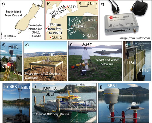
Table 2. Equipment setup at each station, cf. Figure 1.

Station	Terrestrial (fixed) or Marine (moving) installation	Receiver / Antenna	Software (acquisition and processing)	Data rate / observation time days (observation time hours) / logging time (UTC)
MNR1	Terrestrial (fixed)	Trimble R10	TSC3 with Trimble Access 2017.00, TBC v.4 & 5	1Hz / 3 days (55 hrs) / 14th 00:00 – 16th 07:00
DUND	Terrestrial (fixed)	Trimble NetR9 / Trimble TRM57971	CORS: PositioNZ-RT data stream	1Hz / ∼3 days (7 hrs longest continuous timeframe*) / continuous *large data gaps at remote logging computer beginning 14th 10:45.
A24Y	Terrestrial (fixed)	U-blox M8 evaluation kit	U-centre v. 18.11	1Hz / ∼3 days (52 hrs) / 14th 03:00 – 16th 07:00
BBR1	Marine (moving)	Trimble R10	TSC3 with Trimble Access 2017.00, TBC v.4 & 5	1Hz / ∼3 days (49.8 hrs) / 14th 05:10 – 16th 07:00
BBL1	Marine (moving)	U-blox M8 evaluation kit	U-centre v. 18.11	1Hz / ∼3 days (53 hrs) / 14th 02:00 – 16th 07:00
TITG	Terrestrial (fixed)	Waterwatch LS1	Tussock Innovation online portal	0.0033 Hz (5 min) / 3 days / continuous
ETTS	Terrestrial (fixed)	Tide Staff	Manual observation	0.0033 Hz (5 min) for 2x12hr periods over 2 days / 14th 21:00-09:10 and 15th 19:10 − 07:00

Our trial was designed in two stages to analyze potential uses for low-cost single-frequency RTK GNSS in the marine environment by investigating: stage 1) horizontal and vertical position quality over a series of baseline lengths to prove the quality of the low-cost data and thus confirm the validity of using the low-cost RTK observations for our stage 2) tide derivation from vertical measurements taken on a floating platform (the vessel moored alongside the wharf).

GNSS and Tide Gauge Station Fieldwork

The low-cost GNSS equipment used for our trials were U-blox M8 evaluation kits and U-center v.18.11 software. The U-blox receivers were configured the same as the settings in Odolinski and Teunissen 2017b to collect GNSS data from L1 GPS, B1 BDS, L1 Galileo and L1 QZSS constellations.

One U-blox station was used as a base (A24Y – Figure 1f), while another was placed onboard the University of Otago’s 12 m long Research Vessel R/V Beryl Brewin (BBL1 – Figure 1h-j). Trimble R10 receivers were used to log dual-frequency GPS and BDS observations at the most distant base station (MNR1 – Figure 1d) and onboard the vessel (BBR1 – Figure 1h-j) for comparative purposes. GPS, GLONASS and BDS were the only available constellations on our Trimble R10 and U-blox setup in 2018. We did not use GLONASS due to the frequency division multiple access (FDMA) issues for ambiguity resolution at the time of writing (c.f. Teunissen 2019). Base station DUND (Figure 1e) transmitted remotely logged Receiver Independent Exchange (RINEX) data. All stations recorded 1 Hz data through as much of the three day trial period as possible. Large data gaps occurred at the DUND CORS station, likely due to issues with data transmission to the remote logging computer. The longest timeframe of continuous data available from DUND was seven hours, other locations observed between 49.8 and 55 h continuously (Table 2).

For positioning analysis in stage 1 various baselines (see Table 3 and those in Figure 2) were used to demonstrate the applicability of low-cost RTK GNSS to marine users who may have access to an existing base setup in a port, a national network (such as the CORS station we used), or by utilizing higher cost equipment a company already owns.

Figure 2. Known baseline demonstration of 3D data quality for stage 1 over 7 hrs: green dots are Easting, blue dots are Northing, red dots are Up, grey bars show number of satellites; a) 7.3 km baseline; b) 27.4 km baseline.

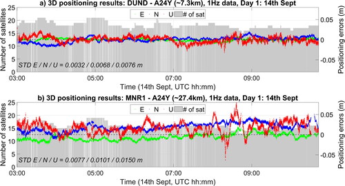
Table 3. Comparison of E, N, U values for different baseline lengths and timeframes for stage 1: Horizontal and vertical position quality checks.

Baseline	Baseline	Baseline timeframe	‘position availability’: % of fixed obs used after 0.1m filtering	Max range: E , N , U (m)	1 sigma standard deviation σ: E , N , U (m)
∼7.3km (Figure 1b, 1e & 1f)	DUND – A24Y	3 days : 14 – 16 Sept (including periods with data gaps at DUND CORS site)	99.8%	0.048 , 0.080 , 0.143	0.006 , 0.009 , 0.016
	DUND – A24Y	1 day : 14 Sept (Figure 2)	99.9%	0.021 , 0.040 , 0.063	0.003 , 0.007 , 0.008
∼27.4km (Figure 1d & 1f)	MNR1 – A24Y	3 days : 14 – 16 Sept	85.3%	0.070 , 0.083 , 0.194	0.009 , 0.010 , 0.022
	MNR1 – A24Y	1 day : 14 Sept (Figure 2)	95.4%	0.045 , 0.063 , 0.143	0.008 , 0.010 , 0.015

For tide derived in stage 2 we used an existing ultrasonic LS1 Remote Water Level Sensor (Tussock Innovation 2018) installed at PML wharf which uses Bluetooth to broadcast tide measurements to an online display at five minute intervals. The tide measurements at this sensor (TITG – Figure 1g) are derived from ultrasonic acoustic readings taken from the sensor to the water surface and converted to local tide values using an installer defined calibration offset. Data from this sensor (TITG – Figure 1g) was collected to be compared with: a) manual in-field observations of the adjacent tide staff (ETTS – also Figure 1g). This comparison confirmed that the sensor (TITG) was recording water height correctly and that the installer defined calibration offset was generating a correct tide value from the sensor measurements; and, b) the vertical RTK GNSS measurements. The tide gauge was less than 20 m from the RTK GNSS antennas onboard the vessel (see Figure 1b inset). As confirmation that the tide gauge was operating correctly, simultaneous manual observations of the adjacent tide staff were undertaken at 5 min intervals for two 12 h periods during the field trials. TITG and ETTS water level height data were then plotted at corresponding times to display their relationship and confirm the appropriate use of the tide gauge as a baseline check for our GNSS derived water heights. During the field trials the weather deteriorated. The resulting drop in air pressure, increasing winds and choppy seas at the PML wharf provided useful environmental variability for our vertical RTK GNSS tide measurement evaluation.

Processing and Analysis

RTK GNSS processing of all data (low- and high-cost) was undertaken using the open source programme package RTKLIB (version 2.4.3 b31). An elevation mask of 10° was used. Geostationary Orbit (GEO) BDS satellite C03 was excluded from processing throughout these trials, as Odolinski and Teunissen (2019, 2016) found the use of the signal from this 12° elevation satellite introduces too much multipath at our southern location. International GNSS Service (IGS) Multi-GNSS Experiment (MGEX) navigation files from Earth Observing System Data and Information System (EOSDIS) of NASA's Earth Science Data Systems (ESDS) Program for the field period were downloaded (from EOSDIS 2018) and used in the RTKLIB baseline processing. In our processing we use the single-epoch (instantaneous) RTK model, with the benefit that the model then becomes insensitive to cycle slips (Odolinski and Teunissen 2017a). Note that this means the time to first fix (TTFF) is always only one epoch. We make use of a double-differenced RTK model with system-specific reference satellites, similar to equation (1)(1) $$\frac{\text{Total \# }\text{of}\mathrm{ }\text{correctly}\mathrm{ }\text{fixed}\mathrm{ }\text{epochs}\mathrm{ }\text{after}\mathrm{ }0.1\mathrm{m}\mathrm{ }\text{low}\mathrm{ }\text{pass}\mathrm{ }\text{filter}}{\text{Total}\text{ \# }\text{of}\mathrm{ }\text{correctly}\mathrm{ }\text{fixed}\mathrm{ }\text{epochs}\mathrm{ }\text{before}\mathrm{ }0.1\mathrm{m}\mathrm{ }\text{low}\mathrm{ }\text{pass}\mathrm{ }\text{filter}}\text{ x }100$$(1) in Odolinski and Teunissen (2016), and the least squares ambiguity decorrelation adjustment (LAMBDA) method is used to fix the full vector of ambiguities to integers (Teunissen 1995).

Filtering, analysis and visualization was completed in MATLAB version R2016a. For both stages data was initially filtered to retain observations with a ‘fixed’ quality flag.

For stage 1 positioning analysis the observation values for E, N and U were subtracted from the average fixed baseline distance, a low pass filter removed values >0.1 m with this used to calculate position availability % (see Equation 1(1) $$\frac{\text{Total \# }\text{of}\mathrm{ }\text{correctly}\mathrm{ }\text{fixed}\mathrm{ }\text{epochs}\mathrm{ }\text{after}\mathrm{ }0.1\mathrm{m}\mathrm{ }\text{low}\mathrm{ }\text{pass}\mathrm{ }\text{filter}}{\text{Total}\text{ \# }\text{of}\mathrm{ }\text{correctly}\mathrm{ }\text{fixed}\mathrm{ }\text{epochs}\mathrm{ }\text{before}\mathrm{ }0.1\mathrm{m}\mathrm{ }\text{low}\mathrm{ }\text{pass}\mathrm{ }\text{filter}}\text{ x }100$$(1) ), the standard deviation for E, N and U calculated and the data plotted.

Only correctly fixed epochs were used in the analysis. For all baselines the ‘position availability’ percentage was calculated as follows: (1) $$\frac{\text{Total \# }\text{of}\mathrm{ }\text{correctly}\mathrm{ }\text{fixed}\mathrm{ }\text{epochs}\mathrm{ }\text{after}\mathrm{ }0.1\mathrm{m}\mathrm{ }\text{low}\mathrm{ }\text{pass}\mathrm{ }\text{filter}}{\text{Total}\text{ \# }\text{of}\mathrm{ }\text{correctly}\mathrm{ }\text{fixed}\mathrm{ }\text{epochs}\mathrm{ }\text{before}\mathrm{ }0.1\mathrm{m}\mathrm{ }\text{low}\mathrm{ }\text{pass}\mathrm{ }\text{filter}}\text{ x }100$$(1)

For stage 2 tide derivation the RTK values for U were extracted, then, taking into account the 2.05 m Spring tide range for the area (LINZ, 2022) we removed RTK observation outliers that were several meters away from the mean of the RTK positions as obvious outliers/incorrect fixes. Finally, in order to illustrate the ability of the low-cost equipment to measure tide we translated RTK observations to the tide gauge datum using a vertical offset between the two which was calculated from the x-axis intercept of a linear trend line fitted between the two; this process was repeated until the vertical offset to be applied converged with less than mm differences to the previous offset iteration. For initial comparison both raw vertical RTK values and tide gauge measurements were plotted against time and then each other (as earlier for the tide gauge and tide staff). Moving average and filtering (5 or 10 min depending on distance to basestation) was then applied to the RTK values and comparisons between results from different baselines plotted. On all tide plots the dual y-axis label recognizes raw RTK data (Vt change) and gauge (Tide) comparison.

Findings for Low-cost RTK GNSS Marine Applications in Otago Harbour Trials

During our work, the low-cost receivers and logging equipment were powered by either one 12v, 24 Ah sealed lead acid battery replaced every ∼24 h or 240 V shore power at PML. Global Kp index values - which indicate disturbances to the earth’s magnetic field and thus influence the ionosphere and GNSS observations (Bartels, Heck, and Johnston 1939) - were downloaded from GeoForschungsZentrum (GFZ), Potsdam, the German Research Centre for Geosciences (https://kp.gfz-potsdam.de/en/https://www.gfz-potsdam.de/en/kp-index/). Matzka et al. describe the three-hourly unitless Kp value notation: ‘Kp = 0o, 0+, 1−, 1o, 1+, …, 9−, 9, where o, + and − represent the integer (o), plus one third (+) and minus one third (−), respectively’ (2021). On this quazi-logarithmic scale a value of 5 indicates a minor geomagnetic storm, 6 a moderate storm etc. (Odolinski and Teunissen 2019). During our observations Kp values ranged from 0+ to 4+ with ionospheric disturbance reducing as the field trials progressed. The number of satellites observed during all aspects of the field trials was generally above 15, with a range of 12 to 21.

Stage 1: Horizontal and Vertical Position Quality

Baseline Easting, Northing and Up values were calculated between the fixed setups DUND and A24Y (baseline ∼7.3 km, see Figures 1b, e & f) and MNR1 and A24Y (baseline ∼27.4 km, see Figure 1d & f) for the entirety of the three day field trial and then over a seven hour time period on the first day – the longest timeframe of continuous data available from DUND due to the data gaps previously mentioned (Figure 2). The average calculated baseline distance was taken from each raw RTK baseline observation and the resulting value plotted as positioning error dots in Figure 2, where East/North/Up position errors are shown as green/blue/red dots over the observation time period along the horizontal axis. The left vertical axis shows the total number of satellites used in the solution, which are then indicated by grey bars running behind the positioning dots across the plot.

As mentioned prior, we hypothesize that the gaps in the DUND data on our second and third days are the result of issues with data transmission from the CORS to the remote logging computer. Data was collected at the U-blox at this time. This missing data affects the three day plot with only 52.6% of the total observations being fixed for the short baseline using DUND compared to 92.8% for the longer baseline which does not use the CORS station (Table 3). Nevertheless, in the data that was able to be logged, this shorter baseline is shown to have a higher position availability after the application of the 0.1 m filter was applied (99.8% vs 85.3% over the 27.4 km baseline seen in column four of Table 3), and more accurate and precise results than those using the longer baseline over 3 days; seen in columns five (max ranges of each of the E/N/U values) and column six (the 1 sigma standard deviation of each of the E/N/U values) of Table 3.

The maximum data ranges are shown to be clearly larger for all E/N/U values (green/blue/red dots on plots) in the longer baseline in Table 3 and Figure 2. In both baselines the red colored Up (U) dots have the largest variation. Table 3 shows that when compared to a calculated average baseline distance, the position observations for the shorter baseline have standard deviation values 1 to 1.5 times smaller than those on the longer baseline.

During the seven hour time period (constrained by the first data gap at DUND) in Figure 2 the data range can be seen to increase on the longer baseline. The shorter baseline in Figure 2 observed more satellites than the longer baseline, likely due to some masking at the MNR1 site. The Up (U) component on the longer baseline is also much larger and more variable, likely due to different atmospheric effects above the antenna as they get further from each other. The shorter baseline had a slightly smaller percentage of ‘fixed’ solutions than the longer (87.7% vs 88.4%), but again a higher percentage of solutions retained after the 0.1 m filter was applied (99.9% vs 95.4%). When compared to the 27.4 km baseline distance, the maximum ranges and standard deviations of the position observations for the 7.3 km baseline are smaller (Table 3). They are also smaller than those for the full 3 day period, likely due to the deterioration of the weather on the 15th and 16th of September which is not included in this seven hour window from the first field day.

Stage 2: Tide Derivation

At PML we undertook a check on the tide gauge (TITG) with two twelve hour observations of the adjacent tide staff (ETTS) (See Figure 1b & g). The heights at corresponding times are plotted as blue dots in Figure 3 with a linear red trend line, and magenta one sigma standard deviation envelope. The plot has the TITG values on the vertical axis and ETTS on the horizontal, with the resulting trend line equation displayed on the plot.

Figure 3. Tide gauge to tide staff observation comparison check using two twelve hour staff reading periods.

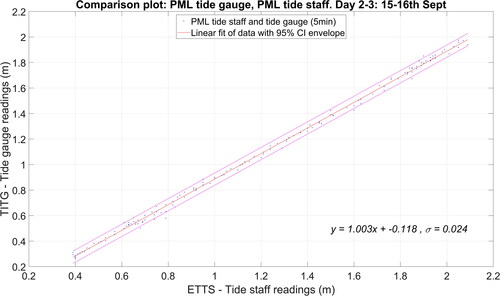
The gradient of +1.003 in Figure 3 demonstrates a strong linear relationship between the vertical observations at the tide gauge and tide staff, while the intercept of −0.12 indicates the tide gauge is logging 0.12 meters lower than the value shown on the adjacent tide staff. If these tide gauge values were to be used further (such as for reducing real-time sounding data to Chart Datum (CD) for nautical publications) then this difference - and the orthometric datum of the tide staff itself - would need to be accounted for (Mills and Dodd 2014). For these trials we are only concerned with observing the accuracy of the vertical movement of the GNSS receiver compared to the nearby gauge, so we can work with the relative vertical movement between sensors, and not consider datum values. The gradient in Figure 4 indicates that the tide gauge was correctly operating and observing what could truly be observed happening (on the tide staff) in the field. Thus, it is suitable to compare the logged tide gauge values with our RTK GNSS derived heights in this location.

Figure 4. Tide derivation from ∼460 m baseline U-blox A24Y – BBL1 (53 hrs): a) Raw U-blox data and PML data; b) U-blox data raw and with gross spike filter plotted with corresponding PML tide gauge data; c) Raw U-blox and five minute moving average U-blox data; d) Five minute moving average U-blox data plotted with corresponding PML tide gauge data. Note: ‘Vt change / Tide (m)’ on y-axis recognizes raw RTK data (Vt change) and gauge (Tide) comparison.

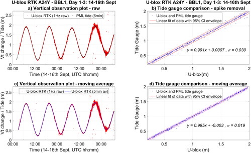
The use and calibration of RTK GNSS heights for tide observation can be envisaged in the same way as the tide staff check described earlier, with Dodd et al. (2009) neatly analogizing RTK GNSS tide measurement as if ‘staff zero is on the ellipsoid’ i.e. our vertical measurements are from the ellipsoid and can be compared in the same way we used our physical tide staff measurements. Our first trial of this used the short ∼460 m long baseline between U-blox receivers A24Y and BBL1 (Figure 4a, see setup in Figure 1b, f & h-j)). In Figure 4 we display the raw BBL2 u-blox data as red dots on the left-side plots with either the raw tide gauge data (TITG) as black dots or the filtered data as a blue line. On the right-side plots we repeat the tide gauge comparison plot (as in Figure 3) with the tide gauge readings on the vertical axis and the u-blox on the horizontal axis. The linear fit is a red line and the one sigma standard deviation shown as a magenta envelope around this. We found that after only applying a gross spike filter the linear correlation between RTK GNSS and the gauge was already strong at 0.991 with a standard deviation of 0.030 (Figure 4b). A five minute moving average further improved this to a gradient of 0.995 and standard deviation of 0.019 (Figure 4c & d). This small standard deviation indicates that correlation coefficients are statistically significant and close to 1.

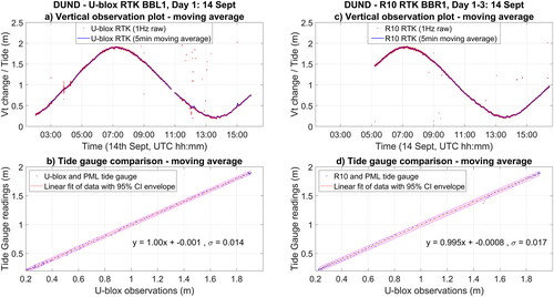
A baseline distance-dependent moving average filter was then applied to the position data collected with the longer baselines using the same vessel based U-blox (BBL1, See Figure 1b & h-j) each time. Figure 5 shows the ∼7.3 km baseline to DUND (See Figure 1b & e) using the same formats as the plots in Figure 4 (but linked vertically instead of horizontally this time), over a sixteen hour period (due to previously discussed base data gaps) with a five minute moving average producing a gradient of 1.000 and standard deviation of 0.014 (Figure 5b). The same baseline from DUND to the Trimble R10 on the vessel (BBR1, See Figure 1b & h-j) that was adjacent to the vessel mounted U-blox (See Figure 1h & j) produced a gradient of 0.995 standard deviation 0.017.

Figure 5. Tide derivation from ∼7.3 km baseline: Low-cost (a&b), R10 (c&d): DUND – U-blox BBL1 (14 hrs): a) DUND - BBL1 raw and five minute moving average; b) Five minute moving average DUND - BBL1 and PML tide gauge data; and, DUND – R10 BBR1 (∼11hrs, note that the R10 did not start logging until 14th Sept 05:10UTC): c) DUND - BBR1 raw and five minute moving average; b) Five minute moving average DUND - BBR1 and PML tide gauge data. Note: ‘Vt change / Tide (m)’ on y-axis recognizes raw RTK data (Vt change) and gauge (Tide) comparison.

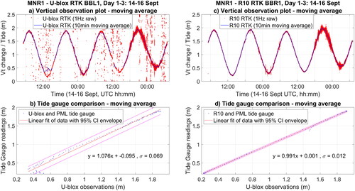
Figure 6 shows the ∼27.4 km baseline to MNR1 (See Figure 1d) over the three day observation period. The low-cost receiver (BBL1) baseline has significantly more noise in the raw data (Figure 6a) with the deteriorating weather clear in the increasing variability from 18:00 on 15th September. With a larger ten minute moving average window, this baseline produces a gradient of 1.076 and standard deviation 0.069 m when compared to the tide gauge (Figure 6b). In comparison, the same length baseline to the Trimble R10 on the vessel (BBR1) is much cleaner in the raw data (Figure 6c), but does have a matching increase in variability on the last 12 h as the weather deteriorated. After applying the ten minute moving average the R10 observations obtain a gradient of 0.991 and standard deviation of 0.012 when compared to the tide gauge (Figure 6d).

Figure 6. Tide derivation from ∼27.4 km baseline with weather deteriorating from ∼18:00 on 15th Sept visible as an increased variability in raw RTK observations: Low-cost (a&b), R10 (c&d): MNR1 – U-blox BBL1 (49.8 hrs): a) MNR1 - BBL1 raw and ten minute moving average; b) Ten minute moving average MNR1 - BBL1 and PML tide gauge data; and, MNR1 – R10 BBR10 (49.8 hrs): c) MNR1 – R10 raw and 10 min moving average; d) Ten minute moving average MNR1 – BBR1 and PML tide gauge data. Note: ‘Vt change/Tide (m)’ on y-axis recognizes raw RTK data (Vt change) and gauge (Tide) comparison.

Discussion

Stage 1: Horizontal and Vertical Position Quality

The first concern when using low-cost RTK GNSS is the quality of the horizontal and vertical position result. The fixed terrestrial combinations (between DUND-A24Y and MNR1-A24Y) shown in Figure 2 and Table 3 demonstrate multi-constellation use with greater than 15 satellites in solutions on both the shorter and longer length baselines. When the number of fixed solutions to total solutions are calculated, both terrestrial baselines (7.3 km and 27.4 km) have >88% success for the times when we had data from all receivers (at other times the CORS station DUND did not record). After filtering we were able to use >85% of the fixed observations for calculations, the lower value indicative of the longer baseline and therefore different relative environments of the receivers, as well as the longer observation period (three days vs seven hours). The standard deviations of Easting and Northing components of the solution were below 0.01 m, with these values decreasing on the shorter baseline. The Up component was predictably larger, but still ≤ 0.016 m standard deviation over the 7.3 km baseline and ≤ 0.022 m standard deviation over the 27.4 km. The benefits of our multi-constellation use are evident by looking at past RTK GPS-only tide buoy trials: Bisnath et al. (2004) investigated RTK GPS buoy observations and compared them to a nearby tide gauge - in a similar manner to our trial - reports an average percentage of suitable RTK solutions (presumed ‘fixed’) of 82%. After one day of observation over a 10 km baseline and filtering with a 12 min moving average, they measured a vertical one standard deviation difference of 0.04 m, decreasing to 0.02 m on a 50 m baseline and increasing to 0.06 m when using two weeks of data over a 15 km baseline (Bisnanth et al. 2004).

Of note is that each baseline in Figure 2 and Table 3 had a low-cost receiver at point A24Y where the final position was calculated, but different receivers and antennas at the base stations MNR1 and DUND (see Table 2). Additionally, the setup at the furthest base, MNR1, had less all-round sky visibility than at DUND and A24Y. By using different receivers for our base stations we give confidence to future users of combined high- and low-cost systems when they are preparing a priori error budgets for hydrographic survey operations. Notwithstanding the previously discussed base station data gaps at DUND, we have shown that horizontal positions are suitable for most hydrographic operations within ∼27.4 km of a base station. Indeed, in many hydrographic operations where it is common to use satellite augmentation system corrections to refine GNSS horizontal positions to around a meter (e.g. European Geostationary Navigation Overlay Service (EGNOS) (ESA 2009)) or decimeter (although up to 0.08 m is mentioned by Fugro MarinestarTM (Fugro 2016)), these low-cost RTK receivers present an affordable and accurate nearshore horizontal positioning alternative.

The Exclusive Order THU in IHO S-44 (2020) allows for ±1 m at 95% confidence level. This is not a challenge for most modern technology, and both of our baselines demonstrate horizontal solutions exceeding this by a factor of 20 or better. This either allows the hydrographer more leniency in the other elements of the total horizontal uncertainty calculation (i.e. offset lever-arm measurement and/or base station location accuracy), or ideally, improves the overall solution such that data will meet or exceed survey standards, and be suitable for modern-day high-accuracy navigation, construction and mapping operations. Of note in the new S-44 standards (2020) is that all other aspects of horizontal positioning for charting also have tighter requirements under the new ‘Exclusive Order’. Some, such as ‘Fixed Objects, Aids, Features Above the Vertical Reference Significant to Navigation’ are now ±1 m at 95% confidence level (half the ±2 m value for the most stringent Special Order in the previous 2008 5th edition version). Thus, use of this single-frequency RTK method would be suitable for other positioning applications beyond depth measurement, and the low-cost equipment may mean a separate survey team could undertake these measurements, potentially speeding up overall survey time.

Similarly, the vertical uncertainties shown on our fixed baselines pass the IHO S-44 Exclusive and Special Order TVU requirements, for depths 10-30 m - see Table 1. Again, this creates the opportunity for the hydrographer to either improve the overall solution of their mapping, or offers more leniency in other vertical measurement components – such as the offset and lever-arm measurements, the derivation of any ellipsoid-geoid relationships used or perhaps even in the precision of the echo-sounder being used.

Stage 2: Tide Derivation

Where geoid-ellipsoid relationships are unknown, or where ellipsoidal surveying is not preferred, tide gauges must be used to correct depth measurements to a local datum. Hydrographers typically confirm the correct operation of a tide gauge by comparing the logged values with water level readings taken at a tide staff near the tide gauge, although checks and calibrations may also be undertaken using observations from a GNSS buoy (LINZ 2020). If the tide staff elevation is connected to known benchmarks (e.g. through levelling runs) or there are known geodetic offsets for the GNSS buoy, then the tide gauge values may be adjusted to provide orthometric heights – we have not done this here, our work undertakes direct comparison with the nearby tide gauge which uses unconfirmed installer calibration values. This is suitable for testing the use of low-cost RTK observations for tide derivation, but further work confirming the tide values would be required if the RTK derived tide values were to be applied to further work – such as in a hydrographic tide reduction. Our results demonstrate the application of both of these check methods; first using the tide staff to check the correct operation of the tide gauge at the PML wharf, and then to compare the moving low- and high-cost GNSS antenna-derived tide (≈ GNSS buoy) to this tide gauge. The distance dependent moving average filter applied to the RTK derived tide after spike removal (Figure 4) created a significantly stronger result and matches the method of averaging that is usually undertaken by traditional tide gauges to remove the effect of high-frequency surface waves. Our results show that simple spike removal and a moving average filter is likely the only further processing needed to generate ultrasonic tide gauge-comparable centimeter accurate real tide data from low-cost RTK observations for use in hydrography and other applications such as engineering or marine science. This may however be location specific, depending on other atmospheric and tidal forcings on sea surface topography that GNSS samplings would also capture or be affected by (see tilt discussion following). A five minute moving average was used for the shorter baseline (Figure 5) and 10 min for the longer (Figure 6). Figure 5 demonstrates that the use of the low-cost antenna (BBL1) produced the same results as the high-cost equipment (BBR1) over the 7.3 km baseline, with the differences between them being sub-centimeter and therefore negligible for RTK methods. Further quality comparisons between U-blox and R10 can be found in Odolinski and Teunissen (2020). The need for filtering single-frequency low-cost GNSS data is shown on the longer baseline in Figure 6, but with the tide gauge comparison one sigma standard deviation around 0.069 m this is still a useful tide measurement. Others using different GNSS receivers (Chorus, Hydrins and CNav) and Precise Point Positioning (PPP) corrections along with local vertical ellipsoid offsets have measured similar average differences than us (∼0.07 m), with their differences likely due to the tide gauge being more distant and their method also including the influence of the uncertainty in the datum model (Dean 2014, Dodd et al. 2009). For our investigation, further levelling runs and/or long-term static GNSS observations in the area would provide us with offset values we could use to transfer our observations into orthometric heights – such as Chart Datum if reducing soundings.

Figure 6 indicates that despites poor or degrading RTK vertical observations (i.e. due to a longer baseline (Figure 6a, b) or in weather deterioration (Figure 6a, b, c, and d)) after a moving average was applied to the data the low-cost RTK observations remained suitable for capturing the tide signal.

Vessel motion, such as pitch and roll, affect the ‘true’ height of any antenna mounted upon them – by reducing the measured height from that when it is truly vertical. In tests on a GPS buoy Dodd et al. (2009) provide calculations to estimate the tilt of the buoy in degrees by using the measured roll and pitch, and applying this to the vertical offset of the antenna from the water surface.

For the duration of our field trials a POSMV Inertial Motion Unit (IMU) mounted at the base of the pole on which the antennas were installed observed mean roll of −0.06°, and pitch of −1.31°. This corresponds with a mean tilt induced vertical antenna height change of 0.0009 m using our vertical antenna offset from the water of 3.54 m. Tilt induced vertical change would become significant if this change was equal to, or greater than, typical vertical RTK precision alone. Trimble quotes ‘±15mm + 0.5 ppm’ for vertical R10’s (2014), which equates to a tilt value of ±5.36° at 1 km from the base station. On the final days when the weather quality decreased (as seen in the red points in Figures 4 and 6), the largest tilt value calculated was 5.18° from simultaneous roll and pitch values of 4.89° and −1.71° respectively so this limit was not reached.

GNSS tide measurement has many benefits. Traditional underwater mounted tide gauges, such as acoustic or pressure sensors, may have issues with power, data transmission and bio-fouling. Surface gauges such as Electronic Distance Measurement (EDM) or Radio Detection and Ranging (RADAR) sensors need stable mounting locations and reliable power sources. Over longer periods of time both can be subject to structure or land subsidence, or large scale tectonic movement. The benefits of GNSS buoys is that they can be deployed in any location without needing to be mounted to fixed equipment. Power, access and maintenance are easier than that for underwater sensors. Results from the ellipsoid will be independent of any of the land or structure movements discussed for traditional gauges (not withstanding tsunami or other waves generated by rapid tectonic earthquakes). Multiple buoys can be set up in a network of locations for a better understanding of co-tidal movement. And in enclosed waters or environments such as on floating ice (Lei et al. 2018), buoys need not even be attached to the seabed, as vertical and horizontal movement can also be used as a measure of tidal flows within the area. Links with ‘Internet of Things’ tide networks and their application to environmental understanding, such as that in Knight et al. (2021), are logical.

As for horizontal and vertical positioning, the use of low-cost RTK GNSS to measure tide has implications for the management of the total vertical uncertainty budget of a hydrographic survey budget. Yet again, any improvement to a component of the vertical uncertainty calculation leads to either higher precision results, or more leniency in other areas of measurement combination. Higher precision may be two-fold; there is the use of low-cost RTK GNSS for directly measuring tide (as in Figures 4–6), but additionally, tidal modeling of a survey area would be made significantly more accurate with the deployment of more low-cost sensors than may currently be achievable with underwater gauges, or high-cost GNSS buoys.

Low-cost RTK GNSS Benefits to Marine Observations

The benefits of low-cost equipment in the marine environment - which is harsh on all electrical equipment - are threefold: smaller physical size, lower power consumption and, when worst happens, cheaper replacement costs. We envisage multiple benefits to hydrographic operations from traditional and novel applications of this low-cost technology. Our work demonstrates that the obtainable data quality, combined with the low-cost equipment outlay make this appropriate for a multitude of applications. Examples of the projects we envisage are: densified tide level networks; use for positioning on traditional vessel setups as well as small Unmanned Surface Vessels (USV) (as in Specht et al. (2019)) or even for surface positioning of Autonomous Underwater Vehicles (AUV); aiding of inertial motion sensors; structure and construction monitoring; measurement improvements at the land/sea interface; and, for use in gathering many more repeatable and robust scientific measurements in the marine environment than may be achieved with high-cost equipment. As an example: Joining Land and Sea (JLAS) is an initiative by Land Information New Zealand (LINZ) to enable datum transformations between, and therefore integration of, terrestrial and marine data (Blick 2018). JLAS requires real-world tide data to improve modelling that will be used for datum transformation calculations. Using low-cost RTK GNSS in this project would add more data to the initial model, and allow further concentrated studies in dynamic tidal areas. Using low-cost RTK GNSS equipment links with other projects working to keep equipment costs down without sacrificing safety (Kraft and Sternberg 2019). The price of the low-cost RTK GNSS equipment compares well with current acoustic tide gauges, quoted at around $7,500USD (Valeport TideMaster) and EDM sensors at around $500USD (HT-0909 ‘radar level gauge’). A ‘low-cost’ acoustic tide gauge was developed in 2000 was quoted at ‘less than $1,500’ (assumed USD) (Giardina et al. 2000).

Future Considerations

Future trials should be done with longer baselines. Vertical measurements used as tide analysis on the longer baseline (∼27.4 km) show the greatest variability when compared to the tide gauge (Figure 6). An increase in baseline length is of use to hydrographers, marine engineers and scientists working further away from base station locations on the coast. Odolinski and Teunissen (2019) have demonstrated the ability the low-cost single-frequency measurements to obtain horizontal standard deviations of 3-16 mm and vertical standard deviations of 8-47 mm over a 9 km baseline in low-to-high periods of ionospheric disturbance. Their trials over a 21.8 km baselines in low ionospheric disturbance performed similarly to the shorter baseline in medium ionospheric disturbance. With these values, analysis of the residual vertical after the removal the tide is possible, leading to heave, dynamic draft and loading derivation (Mills and Dodd 2014). Further tests could also be undertaken with multi-frequency low-cost receivers to understand the accuracy improvements and baseline length increases possible with this equipment (Odolinski and Teunissen 2020).

While comparison plots (Figures 4b, d, 5b, d, 6c, d) indicate low-cost vertical RTK observations are a suitable method for tide calculation, we could further quantify the method by evaluating positioning availability as we have done in Equation 1(1) $$\frac{\text{Total \# }\text{of}\mathrm{ }\text{correctly}\mathrm{ }\text{fixed}\mathrm{ }\text{epochs}\mathrm{ }\text{after}\mathrm{ }0.1\mathrm{m}\mathrm{ }\text{low}\mathrm{ }\text{pass}\mathrm{ }\text{filter}}{\text{Total}\text{ \# }\text{of}\mathrm{ }\text{correctly}\mathrm{ }\text{fixed}\mathrm{ }\text{epochs}\mathrm{ }\text{before}\mathrm{ }0.1\mathrm{m}\mathrm{ }\text{low}\mathrm{ }\text{pass}\mathrm{ }\text{filter}}\text{ x }100$$(1) for the fixed positioning analysis using instantaneous tide gauge values as a benchmark.

More work is required to analyze the effects of multipath when the low-cost equipment is used near highly reflective surfaces such as the water and on the top of metal vessels – often in less optimal mounting locations (such as amongst other navigation equipment). The ground-planes used with our U-blox are 15 cm in diameter (see Figure 1) to aid positioning on 5/8” threads and minimize reflections. No grounding plane was used for the Trimble R10 receivers.

Practically, investigations using solar power or chained batteries to support longer U-blox campaigns would further determine their applicability for long term campaigns, with power consumption in tide networks an element noted by others such as Knight et al. (2021).

Conclusions

The use of RTK GNSS in hydrographic surveying has been considered since the late-1980s and tested from the 1990s with the benefits of measuring tide with GNSS surface buoys being analyzed since GPS and GLONASS were the only constellation available (DeLoach and Remondi 1991, Wells and Kleusberg 1992, DeLoach 1995, Bishanth et al. 2004, Bisnath et al. 2004, Dodd and Mills 2011, Mills and Dodd 2014). This paper modernizes the conversation with the use of multi-constellation, low-cost receivers processed using the single-epoch RTK model, with the benefit that the model then becomes insensitive to cycle slips (Odolinski and Teunissen 2016). We find that for low-cost single frequency RTK GNSS:

1. Stationary horizontal positioning exceeds the highest Exclusive Order requirement in the current IHO S-44 specifications, at different base station ranges up to 27km.

2. Vertical observations are suitable for floating surface-tide measurement and are comparable with electronic tide gauges observations at different base station ranges, although uncertainty will increase on the longer base station ranges (ours was ∼27.4km) when more measurement filtering is required.

3. All of the measurements in 1-2 above will result in improvements to the total uncertainty calculations undertaken by hydrographers. For depth measurements that are comprised of a combination of measurements this means a more precise THU and TVU result can be obtained, or that other elements of the total horizontal and vertical uncertainty calculation can be relaxed – perhaps opening up more options for alternate equipment use or methodologies.

Acknowledgements

The authors thank two anonymous reviewers for suggestions that improved the manuscript. Many thanks are due to Doug Mackie and his team of Sean Heseltine, Dave Wilson, Linda Groenewegen and Andrew Nicolson at the University of Otago’s Portobello Marine Lab (PML), as well as Alastair Neaves, Mike Denham and Nigel Goulstone from the National School of Surveying for their assistance and support during fieldwork. We gratefully acknowledge supportive education and research licenses for Trimble Business Centre (TBC) 4.00, MATLAB R2016a and ArcMap 10.5.1 that enabled our work on this paper. Open source GNSS processing package RTKLIB (v.2.4.3 b31 © T. Takasu) was used under 2-Clause BSD License for all baseline processing (http://www.rtklib.com/).

Disclosure statement

No potential conflict of interest was reported by the author(s).

Data availability statement

The data that support the findings of this study are available from the corresponding author, Emily Tidey, upon reasonable request.

References

- Alkan, R. M., I. M. Ozulu, V. Ilçi, and M. Kahveci. 2015. Single-baseline RTK GNSS Positioning for Hydrographic Surveying. In EGU General Assembly, Vienna, Austria. 1 April 2015.
- Bartels, J., N. H. Heck, and H. F. Johnston. 1939. The three-hour-range index measuring geomagnetic activity. Journal of Geophysical Research 44 (4):411–54.
- Bishanth, S., D. Wells, S. Howden, D. Dodd, and D. Wiesenburg. 2004. Development of an operational RTK GPS-equipped buoy for tidal datum determination. International Hydrographic Review 5 (1):54–64.
- Bisnath, S., D. Wells, M. Santos, and K. Cove. 2004. Initial results from a long baseline, kinematic, differential GPS carrier phase experiement in a marine envrionment. In PLANS 2004. Position Location and Navigation Symposium (IEEE Cat. No.04CH37556) , 26–9 April 2004
- Blick, G. 2018. Joining New Zealand land and sea vertical datums (JLAS). XXVI FIG Congress , Istanbul, 6–11 May 2018.
- Brissette, M. 2012. Stop using DGPS! The unsuitability of non-centimetric positioning for shallow-water MBES surveys. Hydro International. Lemmer, The Netherlands: Geomares.
- Canter, P., and L. Lalumiere. 2005. Hydrographic surveying on the ellipsoid with inertially-aided RTK. Applanix. https://www.applanix.com/pdf/POSMV_2005_09_HydrographicSurveying.pdf.
- Clare, M. A., M. E. Vardy, M. J. Cartigny, P. J. Talling, M. D. Himsworth, J. K. Dix, J. M. Harris, R. J. Whitehouse, and M. Belal. 2017. Direct monitoring of active geohazards: Emerging geophysical tools for deep‐water assessments. Near Surface Geophysics 15 (4):427–44.
- Cohn, N., D. L. Anderson, T. Susa, P. Ruggiero, D. Honegger, and M. Haller. 2014. Observations of intertidal bars welding to the shoreline: Examining the mechanisms of onshore sediment transport and beach recovery. Proceedings of the American Geophysical Union , Fall Meeting 2014, San Francisco, CA, USA, 15–9 December 2014.
- Dabove, P. 2019. The usability of GNSS mass-market receivers for cadastral surveys considering RTK and NRTK techniques. Geodesy and Geodynamics 10 (4):282–9.
- Dean, B. 2014. Evaluation of GNSS-derived tidal information in hydrographic applications. In Hydro14, Aberdeen, Scotland, 28–30.
- DeLoach, S. R., and B. Remondi. 1991. Decimeter positioning for dredging and hydrographic surveying. In 6. Fort Belvoir, VA: US Army Topographic Engineering Center.
- DeLoach, S. R. 1995. GPS tides: A project to determine tidal datums with the global positioning system. M.Eng report, Department of Geodesy and Geomatics Engineering Techical Report No. 181, University of New Brunswick, Fredericton, New Brunswick, Canada, 105.
- Dodd, D., and J. Mills. 2011. Ellipsoidally referenced surveys: Issues and solutions. International Hydrographic Review 6:19–29.
- Dodd, D., B. Mchaffey, G. Smith, K. Barbor, S. O-Brien, and M. van Norden. 2009. Chart datum transfer using a GPS tide buoy in Chesapeake Bay. International Hydrographic Review (2):39–51.
- Earth Observing System Data and Information System (EOSDIS). 2018. Multi-GNSS Experiment (MGEX) Navigation Files . NASA's Earth Science Data Systems (ESDS) Program. ftp://ftp.cddis.eosdis.nasa.gov/gnss/data/campaign/mgex/daily/rinex3/2018/brdm
- Eeg, J. 2004. Verification of the Z-Component in the RTK survey of Drogden Channel. The International Hydrographic Review 5 (2):16–25.
- Elsobeiey, M. 2017. Performance analysis of low-cost single-frequency Gps receivers in hydrographic surveying. The International Archives of the Photogrammetry, Remote Sensing and Spatial Information Sciences XLII-4/W5:67–71.
- European Space Agency (ESA). 2009. EGNOS: European Geostationary Navigation Overlay Service. In. www.esa.int/EGNOS. Online pdf.
- FIG (International Federation of Surveyors) Commission 4. 2010. Guidelines for the planning, execution and management of hydrographic surveys in ports and harbours. In FIG Publication 56. edited by Working Group Hydrographic Surveying in Practice. Copenhagen, Denmark: International Federation of Surveyors (FIG).
- Fugro. 2016. MarineStarTM positioning services. Leidschendam, Netherlands: Fugro.
- Giardina, M. F., M. D. Earle, J. C. Cranford, and D. A. Osiecki. 2000. Development of a low-cost tide gauge. Journal of Atmospheric and Oceanic Technology 17 (4):575–83.
- He, H. 2010. Quality control of GPS RTK technology in road engineering. 2010 International Conference on Mechanic Automation and Control Engineering, Wuhan, China, 26–28 June 2010.