Automatic Detection and Analysis of the Shoreline Change Rate at Maravanthe Coast, India

Abstract

Maravanthe Beach has been witnessing erosion due to waves caused by tidal forces, destroying vegetation, and causing enormous damage to people’s lives, livestock, and property. Hence, an attempt has been made to understand the shoreline change analysis using the automatic shoreline extraction method and determine the rate of change in terms of erosion and accretion rate before and after the construction of coastal structures during the period from 2014 to 2023. The SWAT model was applied to analyze the influence of surface runoff on shoreline changes near Maravanthe Beach for the periods 2004–2014 and 2012–2023. Also, runoff was chosen as one of the parameters for validation of the analysis. It was noticed that the shoreline stretch had experienced significant erosion prior to the construction of shore protection infrastructure. Soon after the deployment of certain shore structures, the shoreline progressed from a high erosion stretch to a low erosion stretch. This study reveals that Maravanthe Beach witnessed greater erosion during the period 2014–2018 than it did from 2019–2023 and also observed a decrease in erosion from 11% to 3% and an increase in the accretion zones from 2 to 9%.

Keywords:

• Landsat-8
• DSAS
• shoreline change
• SWAT
• SWATCUP

Introduction

The lithosphere, cryosphere, atmosphere, and hydrosphere are various components that connect together to establish one cohesive system influencing the global ecological system with multiple inter-relationships between biotic and abiotic elements. These relationships include interactions with soil, ocean, water, solar radiation, and climate. Even a single imbalanced climate variable in nature or anthropogenic activities have a direct/indirect impact on both the environment and human life (Chahine 1992). Urbanization and industrialization along the coastal belt have impacted coastal settings over time, changing the shoreline and upsetting coastal ecosystems. Every nation with areas of coastline faces challenging circumstances as a result of high tides, cyclones, coastal tourism, pollution from industrial waste disposal, construction of harbors, etc. all of which have an adverse effect on the natural coastal ecosystems (Davis, Finkl, and Makowski 2019; Sempere-Valverde et al. 2023).

India’s coastline is 7516.6 km long, divided into 5422.6 km of main coastal zone landforms and 1197 km of Indian islands coastline. An analysis of shoreline change using satellite images from 1990 to 2016 by the National Centre for Coastal Research under the Ministry of Earth Sciences estimated that 34% of the coastlines were eroded, 28% had accretion, and 38% were stable over the period (Kankara, Ramana Murthy, and Rajeevan 2018). In addition to sea level rise, the coastal regions of India have encountered issues/challenges due to the liberalization of coastal laws, urbanization, the inadequacy of scientific data and regulatory frameworks, and the inadequate capacities of municipal councils (Ramachandran 1999). In order to reduce the adverse effects of shoreline changes, it is vital to identify various factors that could influence natural coastal processes or man-made activities affecting beach morphology. Additionally, mitigation entails the choice of appropriate techniques for evaluating the shoreline, use of appropriate coastal management strategies, design, collection of data (including satellite data and field data), analysis and interpretation of the results, and use of collected data in the creation of early warning systems so as to be well-prepared in the event of extreme erosion or other calamities (Leatherman 2003). Also, the construction of a dam across the river plays a huge negative role in beach morphology (Anthony, Almar, and Aagaard 2016, Pagán et al. 2017 and Yadav, Dodamani, and Dwarakish 2022) by retaining sediment flux within the reservoir which leads to an imbalance in the sediment conveyor belt and reduced supply of sediment to the coast (Syvitski et al. 2005) On the other hand, natural and man-made are also responsible for sediment dynamics such as the type of beach, its geology, wind and wave parameters, and the deployment of a groyne and a breakwater (Bio et al. 2022). The river flood factor also plays a major role in the case of coastal zone protection, river flood characteristics can be better predicted by using the 1D/2D HEC-RAS hydraulic model (Samarasinghe et al. 2022).

The deployment of various coastal management measures, as well as the causes and effects of shoreline alterations, are all analyzed and discussed in the past literature (Cicin-Sain 1993; Olsen and Christie 2000; Westmacott 2002). Previously, field-based topographic surveys were undertaken to analyze beach profiles and shoreline settings (Yang and Li 2012). With the advent of aerial imagery acquisition tools, researchers now use light detection and ranging (LIDAR), satellite observation, and remote sensing products to monitor and assess changes in beach/shoreline morphology (Skilodimou et al. 2021, Yang and Li 2012) and also river morphology (Basnayaka et al. 2022). It is very important to analyze the shoreline historically and predict the substantial variations in the coastal zone before implementing any sustainable plans (Fernández-Hernández et al. 2023). In recent years, several approaches and algorithms have been developed to detect shoreline changes. For instance, methods such as histogram equalization, adaptive thresholding, and automatic thresholding algorithms based on histogram segmentation have been proposed for automated shoreline extraction (Kuleli et al. 2011; Aedla, Dwarakish, and Reddy 2015). Additionally, many open-source software tool kits like CoastSat (Vos et al. 2019) and the Shoreline extraction tool (Daniels 2012) have been utilized to analyze sandy coastlines. A systematic literature review was conducted by Rahman, Crawford, and Islam (2022) on articles (published between 2000 and 2021) that used geospatial techniques (such as remote sensing and GIS) to analyze shoreline change. The Digital Shoreline Analysis System (DSAS) and geographic information system (GIS) were found to be the most commonly used geospatial techniques for detecting shoreline changes (Boussetta et al. 2022). Recently, (Gireesh et al. 2023) implemented an object-based approach to extract and detect shoreline changes from Landsat-8 imagery of the Visakhapatnam–Kakinada coast along India’s east coast. For the short-term shoreline analysis or for coastal zone monitoring Sentinel-2 time series shows good response and sandy shoreline detection potentially carried by semi-automatic methods such as object-based image analysis (OBIA) and random forest (RF) (Boussetta et al. 2023) and rocky shoreline extracted using object-based image analysis (OBIA) and Convolutional neural network (CNN) (Bengoufa et al. 2021). This object-based approach used the feature extraction workflow by considering maximum likelihood in the maximum classification method (MLC) to automatically detect the coastline from Landsat imagery. Likewise, the evolution of the coastal zone along the northern part of the Sebou estuary from 1984 to 2021 was analyzed (Ennouali et al. 2023) using Landsat images and the DSAS tool. The DSAS tool provides analysis of various results such as including Shoreline Change Envelope (SCE), Net Shoreline Movement (NSM), End Point Rate (EPR), and Linear Regression Rate (LRR) (Zoysa et al. 2023)

By conducting shoreline change mapping, it becomes possible to prevent damages from potential future events through the implementation of effective mitigation measures by the relevant authorities (Yadav, Dodamani, and Dwarakish 2021; Yadav, Dodamani, and Dwarakish 2022). The region (Maravanthe coast) under investigation in this study experiences significant shoreline erosion caused by both natural and human-induced factors. It is crucial to assess and monitor this erosion to mitigate the loss of life, property, and business, as well as to protect and promote the tourism industry. The study area has witnessed the detrimental effects of erosion, which include vegetation loss, damage to individual property, livestock, etc. caused by tidal waves. Therefore, this study aims to analyze the changes in shoreline dynamics, specifically erosion and accretion rates, before and after the construction of coastal structures between 2014 and 2023. An innovative aspect of this study is that it considers the shoreline change analysis before and after beach groin construction (shoreline armoring structures) and gives a better insight into the advantage of it.

Study Area

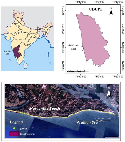
Udupi District is the coastal district of Karnataka state that comprises three taluks namely Udupi, Kundapur, and Karkala with a total geographic area of 3575 square km. The study area extends from Trasi to Maravanthe village present in Byndoor taluk. The area lies between Latitude and Longitude of 13° 41′ 14.44″ N, 74° 38′ 39.76″ E to 13° 43′ 7.05″ N, 74° 38′ 24.29″ E as shown in Figure 1. This place is famous and unique because National Highway 66 runs alongside the Arabian Sea on one side and the Souparnika River on the other side. The road that runs alongside the sea experiences negative impacts from the coast, with seawater splashing the highway and the coastline eroding drastically. These events failed to attract the attention of the government organizations until strong waves and tidal forces washed away parts of the road, shore-land, and footpath interlocking tiles all along the shoreline. The coastal stretch along Maravanthe Beach was subjected to erosion, so seawalls with no proper design were constructed along the coast to protect the road and human properties from harsh waves and sea-level rise. However, these seawalls were ineffective and only provided temporary protection. In 2016, the Sustainable Coastal Protection and Management Investment Program (SCPMIP)-Project 2 executed a new project to address the coastal erosion along Maravanthe Beach. After assessing many alternatives, the project team concluded that the best way to reduce further erosion and maintain stability at the beach was to construct groins. Groins are structures that extend out into the water from the shoreline. They work by trapping sand that would otherwise be carried away by waves (Badiei, Kamphuis, and Hamilton 1995). In this project, 7 and 8 straight groins were constructed in the northern and southern sections of the beach, respectively, with 120 m and 150 m spacing center to center, correspondingly. A total of 9 T-Head groins were also constructed in the middle section, with 150 m spacing center to center. The project was completed in 2020, and the results have been promising. The groins have helped to reduce erosion and maintain stability at the beach (Yadav 2017).

Figure 1. Study area: Maravanthe beach.

Methodology

An attempt was made to understand the shoreline change analysis regarding erosion and accretion rates before and after the construction of coastal structures during the period from 2014 to 2023. The methodology of the work was solely dependent on the objective of the study. It was carried out in two phases. The first phase involved the analysis of shoreline change and the mapping of shorelines into erosion and accretion zones. The second phase focused on finding out the effect of runoff on shoreline change, which was done with the help of the Soil and Water Assessment Tool (SWAT). In this study, Landsat 8 OLI_TIRS multi-temporal satellite data that contains atmospherically corrected surface reflectance and land surface temperature derived from the data produced by the Landsat 8 OLI/TIRS sensors for the period 2014–2023 to observe shoreline change for two periods: 2014–2018 and 2019–2023, which represent the periods before and after the construction of coastal structures. Shorelines were automatically digitized in the ArcGIS 10.4 environment. While the Satellite images were obtained (downloaded) from USGS Earth Explorer https://earthexplorer.usgs.gov and Bhuvan geospatial data https://bhuvan.nrsc.gov.in. The Satellite data information used is provided in Table 1.

Table 1. Source of data.

Sl No.	Satellite & sensor	Date of acquisition	Acquisition time	Path /Row
1	Landsat-8 OLI/TIRS	2014/03/29	2014:05:23:12	146/51
2	Landsat-8 OLI/TIRS	2015/04/01	2015:05:21:58	146/50
3	Landsat-8 OLI/TIRS	2016/03/18	2016:05:22:22	146/51
4	Landsat-8 OLI/TIRS	2017/03/21	2017:05:22:37	146/51
5	Landsat-8 OLI/TIRS	2018/03/24	2018:05:22:04	146/51
6	Landsat-8 OLI/TIRS	2019/03/27	2019:05:22:07	146/51
7	Landsat-8 OLI/TIRS	2020/03/29	2020:05:22:17	146/51
8	Landsat-8 OLI/TIRS	2021/04/01	2021:05:22:20	146/51
9	Landsat-8 OLI/TIRS	2022/04/04	2022:05:22:19	146/51
10	Landsat-8 OLI/TIRS	2023/03/30	2022:05:22:31	146/51

Shoreline Analysis

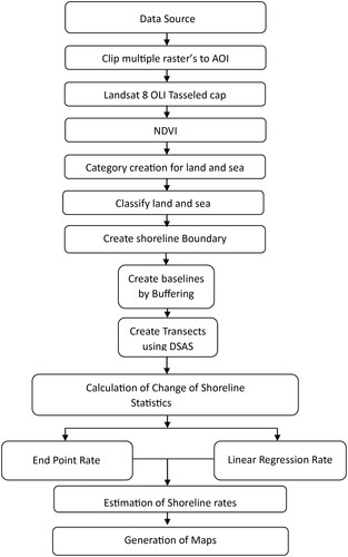
Extraction of shoreline is a crucial part of any shoreline change detection study. Shorelines can be extracted from multi-spatio-temporal data in either raster or vector format. Different types of satellite imagery could be used to extract shorelines using manual, semi-automatic, or automatic methods. In this study, automatic digitization was used with the help of a shoreline extraction tool (DSAS) that is freely available and can be used in ArcGIS 10. To reduce the tedious task of extracting shorelines, a model was built using ESRI's Model Builder. The model was used to create a toolbox for extracting shorelines from different Landsat satellite data sets. This model automates many of the monotonous tasks involved in working with Landsat datasets (Daniels 2012, Eken and Sayar 2015). The shoreline extraction tool is freely available and can be added from the Arc toolbox. Multiple shorelines can be extracted automatically in the ArcGIS environment. The methodology is explained in the flowchart (Figure 2) shown below. The Digital Shoreline Analysis System (DSAS) is a software plugin that works within the ArcGIS software platform (Himmelstoss et al. 2018). DSAS calculates rate-of-change statistics for a time series of shoreline vector data. This study used Landsat 8 OLI/TIRS images from 2014 to 2023. After automatically digitizing shorelines for different periods from 2014 to 2023, the individual extracted shoreline features were put together into a single shapefile. The baseline is a starting point that can be onshore, offshore, or mid-shore. Transects are cast perpendicular (orthogonal) to the baseline at a user-defined spacing and intersect the shorelines to establish measurement points on one or both sides of the baseline. Shoreline change statistics are computed using shoreline cover envelope, weighted linear regression, net shoreline movement, end point rate, and linear regression rate. In this study, the linear regression rate (LRR) and end point rate (EPR) statistical approaches were used.

Figure 2. Flow chart of shoreline analysis.

Validation of Shoreline Change

The shoreline is not only affected by natural processes like wind, waves, and tides, but also by indirect factors such as climate change, sea-level rise, seasonal variations in runoff, and human interventions. Estuaries are one of the most important ecosystems as they provide a home to many species and help to filter out sediments and pollutants from water. Estuaries are likely to be influenced by seasonal variations and climate change, which in turn can raise sea level and change runoff patterns (Kennish 2002).

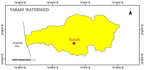
In this study, runoff was used as one of the parameters to validate shoreline changes. The methodology was divided into two phases: simulation of runoff at the Haladi station and subsequent analysis using calibrated parameters in the neighboring ungauged basin. The Haladi gauging station lies in Varahi watershed which is located in the Udupi district of Karnataka, India. It has a latitude of 13° 34′ 55.2" and a longitude of 75° 0′ 3.6". As shown in Figure 3, the Varahi watershed has a natural flow system, which makes it easier to analyze the flow that affects runoff generation. The SWAT model was used to simulate runoff in the watershed, and the calibrated parameters from the model were then used to predict runoff in the neighboring ungauged basin.

Figure 3. Varahi watershed.

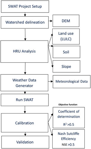
The SWAT is a physically based model that is widely used for both large and small watersheds. SWAT can be used to estimate runoff, sediment, and nutrient yields, and to assess the impact of land use and land management practices on water quality and quantity. The model requires some inputs, such as digital elevation data, land use data, soil data, and weather data. These inputs can be easily obtained from public sources, and SWAT can be used to simulate water and sediment flows for long periods of time (Arnold and Allen, 1999, Gassman et al. 2007). As mentioned, datasets for the SWAT model were collected. The analysis was then carried out in two stages, as shown in Figure 4.

Figure 4. Flowchart of SWAT analysis.

The first step in estimating runoff is to collect data from various sources for input into the SWAT model. The data required is collected and Table 2 shows a description of the data collected.

Table 2. Description of data collected for SWAT analysis.

Data	Source	Description
DEM	Bhuvan website	Product Cartosat-1 DEM-version-3R1, resolution 30 m
LULC	USGS Earthexplorer (2014) Esri Inc. (2020)	The Terra & Aqua combined Moderate Resolution Imaging Spectroradiometer (MODIS) land cover type Derived from ESA sentinel imagery at 10 m resolution
Soil	FAO soils portal	Digital soil map of the world
Weather Data	Arc-SWAT website (2004 − 2014) NASA power (2015–2020)	Global weather data includes Precipitation and Temperature data
Discharge Data	Water resource information system (WRIS), India	Daily river discharge data from 2004 to 2020

• Stage 1: The SWAT model is set up and run for the period of 2004–2014, with the simulation warm period (NYSKIP) of 2 years. The model is run on a daily timescale. A program named SWAT-CUP, developed by Abbaspour et al. (2007), can be used to execute the calibration of SWAT models. Calibration and validation are accomplished by using SWAT-CUP to compare daily simulated flows with observed stream flows at the Haladi gauge station. The parameters are calibrated to obtain a good fit model response, and the calibrated parameters are then used to simulate runoff in an ungauged basin. The observed discharge information was obtained from the Indian WRIS website. In this study, the Sequential Uncertainty Fitting (SUFI) method was used for calibration and validation. SUFI 2 is a computationally intensive method that requires many iterations, typically around 1000 iterations. Calibration was carried out for the period 2006–2011, and validation was carried out for the period 2012–2014.

• Stage 2: After calibration, the same calibrated parameters were used as initial parameters in SWAT for the years 2014 and 2023 in the ungauged watershed. An ungauged station located near the beach, 27 km away from the Haladi station, was chosen for analysis. To check the performance of the model, graphs were drawn between the observed and simulated data. The strength of calibration and uncertainty measures were also evaluated. The objective function R² (coefficient of determination) was chosen to assess the performance of the model on a daily basis.

Results and Discussion

The shoreline shift towards landwards or seawards before and after the construction of armoring structures at Maravanthe Beach was analyzed. The period of 2014–2018 was considered as before and 2019–2023 as after the construction of coastal structures like breakwaters and groins. Two statistical methods, namely end point rate (EPR) and linear regression rate (LRR), were used for the analysis of the rate of change. Maps were created to visualize the results.

Shoreline Dynamics During the Period of 2014–2018

The 12-kilometer-long Maravanthe Beach shoreline was automatically delineated from satellite imagery of different years (2014–2018) using the shoreline extraction tool. The rate of change was found using statistical methods such as end point rate (EPR) and linear regression rate (LRR) in terms of erosion and accretion. Negative and positive values indicate erosion and accretion, respectively.

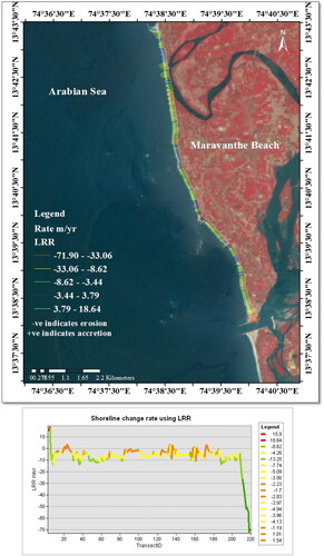
According to the results obtained from EPR (Figure 5), the erosion rate was observed to be as high as −81.5 m/yr and as low as −0.02 m/yr, while the accretion rate was observed to be as high as +18.56 m/yr and as low as +0.08 m/yr. Similarly, according to the results obtained from LRR (Figure 6), the erosion rate was observed to be as high as −71.90 m/yr and as low as −0.28 m/yr, while the accretion rate was observed to be as high as +18.64 m/yr and as low as +0.2 m/yr. Both statistical methods showed that the area was more prone to erosion than accretion. The average shoreline rate of change was +0.08 m/yr (LRR) and +0.08 m/yr (EPR).

Figure 5. EPR map of the study area for 2014–2018.

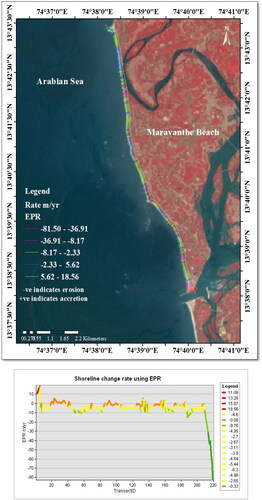
Figure 6. LRR map of the study area for 2014–2018.

Shoreline Dynamics during the Period of 2019–2023

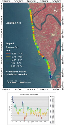
After the construction of coastal structures was completed, the years 2019–2023 were used to study shoreline change. The maps are plotted to show the rate of change during this period, after the construction of coastal structures. The maximum erosion rate observed was −7.18 m/yr, and the minimum was −0.54 m/yr. The maximum accretion rate was 12.38 m/yr, and the minimum was 2.06 m/yr. The average shoreline change rate was 0.24 meters per year. Figure 7 shows the EPR map. Similarly, according to the results obtained from LRR (Figure 8), the erosion rate was observed to be as high as −8.25 m/yr and as low as −0.97 m/yr, while the accretion rate was observed to be as high as 13.04 m/yr and as low as 1.67 m/yr. The coastal length of Maravanthe Beach is approximately 12,237.2 kilometers. According to shoreline change analysis of the area from 2014 to 2018, 11% of the coast was eroding and 2% was accreting. In 2019–2023, the erosion rate decreased to 3% and the accretion rate increased to 9%. This represents a decrease in erosion of 9% and an increase in accretion of 7%.

Figure 7. EPR map of the study area for 2019–2023.

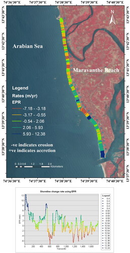
Figure 8. LRR map of the study area for 2019–2023.

The analysis found that before the construction of groins, the area was dominated by erosion, which had negative impacts on transportation, tourism, and lives. The construction of groins appears to have helped to decrease erosion and increase accretion, which has reduced the negative impacts on the surrounding environment.

Analyzing the Influence of Surface Runoff on Shoreline Changes

This section highlights the results obtained at each step during the modeling, calibration, and validation process using the SWAT and SWAT-CUP models. The calibration process was carried out using the SWAT CUP model. Calibration was done for six years starting from 2006 to 2011. Iterations were done until good fit results were obtained, and this occurs when simulated results match with observed data values. The sensitivity analysis was carried out to identify the most sensitive parameters, which were then adjusted to improve the calibration.

On comparison of simulated flow values with observed discharge, the R² and NSE values of 0.734 and 0.54, respectively indicate that the model was able to simulate the discharge data reasonably well. Validation was done for the period 2012–2014 to determine the accuracy of the model results after calibration. The values of R² and NSE after validation were 0.83 and 0.73, respectively. The R² value indicates the degree of correlation between the simulated and observed data, while the NSE value indicates the efficiency of the model in simulating the observed data. In this case, the R² value of 0.83 indicates that there is a strong correlation between the simulated and observed data, while the NSE value of 0.73 indicates that the model is efficient in simulating the observed data.

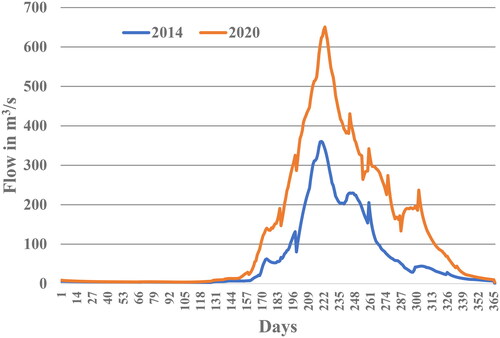
To analyze the influence of surface runoff on shoreline changes between the years 2014 and 2023, a comparison graph (Figure 9) was plotted between the two periods. The graph shows that the flow m³/s was higher in 2020 than in 2014. This suggests that surface runoff may have played a role in the shoreline changes that occurred between the two years. The higher flow in 2020 suggests that there was more surface runoff that year. Naturally, surface runoff carries the sediments along with itself. The sediment transport from river/surface runoff was essential for beach nourishment. This could have benefited the shoreline to accretion more in 2020 than in 2014. However, it is important to note that other factors may also have contributed to the shoreline changes. For example, the tides and currents may have also played a role. More research is needed to determine the exact cause of the shoreline changes.

Figure 9. Flow comparison graph of period 2014 & 2020.

Conclusions

This study found that Maravanthe Beach was subjected to more erosion in the period 2014–2018 than in 2019–2023. The erosion rate decreased from 11 to 3%, and the accretion zones increased from 2 to 9%. This suggests that the construction of groins may have helped to reduce erosion and increase accretion. The increased surface runoff in 2020 could have offset some of the benefits of the groins. However, the overall trend is still towards a decrease in erosion and an increase in accretion. This study provides some evidence that groins can be an effective way to reduce erosion and increase accretion. The increase in runoff generation could be affected by land use, soil properties, land slope, and rainfall intensity.

Author contributions

Conceptualization, A.Y. and C.G.H; methodology, A.Y.; software, S.M; validation, A.Y., and C.G.H.; formal analysis, S.M.; investigation, S.M.; data curation, S.M. and A.Y.; writing—original draft preparation, S.M., A.Y. and C.G.H.; writing—review and editing, A.Y.; visualization, S.M. and A.Y.; supervision, N.H.N. All authors have read and agreed to the published version of the manuscript.

Acknowledgment

This research received no external funding.

Disclosure statement

No potential conflict of interest was reported by the author(s).

Data availability statement

Data will be made available upon request.

References

- Abbaspour, K. C., M. Vejdani, S. Haghighat, and J. Yang. 2007. “SWAT-CUP Calibration, and Uncertainty Programs for SWAT.” In Proceedings of the MODSIM 2007 International Congress on Modelling and Simulation. Modelling and Simulation Society of Australia and New Zealand Inc, (MSSANZ). 1596–1602. ISBN : 978-0-9758400-4-7
- Aedla, R., G. Dwarakish, and D. V. Reddy. 2015. “Automatic Shoreline Detection and Change Detection Analysis of Netravati-Gurpur River Mouth Using Histogram Equalization and Adaptive Thresholding Techniques.” Aquatic Procedia. 4: 563–570.
- Anthony, E. J., R. Almar, and T. Aagaard. 2016. “Recent Shoreline Changes in the Volta River Delta, West Africa: The Roles of Natural Processes and Human Impacts.” African Journal of Aquatic Science 41 (1): 81–87. https://doi.org/10.2989/16085914.2015.1115751
- Arnold, J. G., and P. M. Allen. 1999. “Automated Methods for Estimating Baseflow and Ground Water Recharge from Streamflow Records.” Journal of American Water Resources Association 35: 411–424.
- Badiei, P., J. W. Kamphuis, and D. G. Hamilton. 1995. “Physical Experiments on the Effects of Groins on Shore Morphology.” In Proceedings of the.” 24th International Conference on Coastal Engineering 1994; Kobe, Japan: American Society of Civil Engineers. 1782–1796.
- Basnayaka, V., J. T. Samarasinghe, M. B. Gunathilake, N. Muttil, D. C. Hettiarachchi, A. Abeynayaka, and U. Rathnayake. 2022. “Analysis of Meandering River Morphodynamics Using Satellite Remote Sensing Data—an Application in the Lower Deduru Oya (River), Sri Lanka.” Land 11 (7): 1091. https://doi.org/10.3390/land11071091
- Bengoufa, S., S. Niculescu, M. K. Mihoubi, R. Belkessa, and K. Abbad. 2021. “Rocky Shoreline Extraction Using a Deep Learning Model and Object-Based Image Analysis.” The International Archives of the Photogrammetry, Remote Sensing and Spatial Information Sciences XLIII-B3-2021: 23–29. https://doi.org/10.5194/isprs-archives-XLIII-B3-2021-23-2021
- Bio, A., J. A. Gonçalves, I. Iglesias, H. Granja, J. Pinho, and L. Bastos. 2022. “Linking Short-to Medium-Term Beach Dune Dynamics to Local Features under Wave and Wind Actions: A Northern Portuguese Case Study.” Applied Sciences 12 (9): 4365. https://doi.org/10.3390/app12094365
- Boussetta, A., S. Niculescu, S. Bengoufa, and M. F. Zagrarni. 2023. “Deep and Machine Learning Methods for the (Semi-) Automatic Extraction of Sandy Shoreline and Erosion Risk Assessment Basing on Remote Sensing Data (Case of Jerba island-Tunisia).” Remote Sensing Applications: Society and Environment 32: 101084. https://doi.org/10.1016/j.rsase.2023.101084
- Boussetta, A., S. Niculescu, S. Bengoufa, and M. F. Zagrarni. 2022. “Spatio-Temporal Analysis of Shoreline Changes and Erosion Risk Assessment along Jerba Island (Tunisia) Based on Remote-Sensing Data and Geospatial Tools.” Regional Studies in Marine Science 55: 102564. https://doi.org/10.1016/j.rsma.2022.102564
- Chahine, M. T. 1992. “The Hydrological Cycle and Its Influence on Climate.” Nature 359 (6394): 373–380. https://doi.org/10.1038/359373a0
- Cicin-Sain, B. 1993. “Sustainable Development and Integrated Coastal Management.” Ocean and Coastal Management. 21: 11–43.
- Daniels, R. C. 2012. “Using ArcMap to Extract Shorelines from Landsat TM & ETM + Data.” In Proceedings of the 32nd ESRI International Users Conference, San Diego, CA. 23–27.
- Davis, R. A., C. W. Finkl, and C. Makowski (Eds.). 2019. “Human Impact on Coasts.” In Encyclopedia of Coastal Science. Eds. Finkl C. W., Makowski C. Cham: Springer International Publishing, 983–991. doi: 10.1007/978-3-319-93806-6_175
- Eken, S., and A. Sayar. 2015. “An Automated Technique to Determine Spatio-Temporal Changes in Satellite Island Images with Vectorization and Spatial Queries.” Sadhana 40 (1): 121–137. https://doi.org/10.1007/s12046-014-0309-7
- Ennouali, Z., Y. Fannassi, A. Benmohammadi, M. Al-Mutiry, and A. Masria. 2023. “Shoreline Change Detection along North Sebou–Moulay Bousselham, Based on Remote Sensing Analysis.” Regional Studies in Marine Science 62: 102935.
- Fernández-Hernández, M., A. Calvo, L. Iglesias, R. Castedo, J. J. Ortega, A. J. Diaz-Honrubia, P. Mora, and E. Costamagna. 2023. “Anthropic Action on Historical Shoreline Changes and Future Estimates Using GIS: Guadarmar Del Segura (Spain).” Applied Sciences 13 (17): 9792. https://doi.org/10.3390/app13179792
- Gassman P W, Reyes M R, Green C H and Arnold J G (2007) “The Soil and Water Assessment Tool: Historical Development, Applications, and Future Research Directions.” Transactions of the ASABE 50 (4): 1211–1250 https://doi.org/10.13031/2013.23637
- Gireesh, B., P. Acharyulu, V. Ch, B. Sivaiah, K. Venkateswararao, K. Prasad, and C. Naidu. 2023. “Extraction and Mapping of Shoreline Changes along the Visakhapatnam–Kakinada Coast Using Satellite Imageries.” Journal of Earth System Science 132: 52.
- Himmelstoss, E. A., R. E. Henderson, M. G. Kratzmann, and A. S. Farris. 2018. Digital Shoreline Analysis System (DSAS) Version 5.0 User Guide (Open-File report 2018–1179). US Geological Survey.
- Kankara, R., M. V. Ramana Murthy, and M. Rajeevan. 2018. National Assessment of Shoreline Changes Along Indian Coast—A Status Report for 1990–2016 (Technical report). Chennai, India: National Centre for Coastal Research.
- Kennish, M. J. 2002. “Environmental Threats and Environmental Future of Estuaries.” Environmental Conservation 29: 78–107.
- Kuleli, T., A. Guneroglu, F. Karsli, and M. Dihkan. 2011. “Automatic Detection of Shoreline Change on Coastal Ramsar Wetlands of Turkey.” Ocean Engineering 38 (10): 1141–1149. https://doi.org/10.1016/j.oceaneng.2011.05.006
- Leatherman, S. P. 2003. “Shoreline Change Mapping and Management along the U.S. East Coast.” Journal of Coastal Research 38( Special Issue): 5–13.
- Olsen, S., and P. Christie. 2000. “What are we Learning from Tropical Coastal Management Experiences?” Coastal Management 28 (1): 5–18. https://doi.org/10.1080/089207500263602
- Pagán, J. I., I. López, L. Aragonés, and J. Garcia-Barba. 2017. “The Effects of the Anthropic Actions on the Sandy Beaches of Guardamar Del Segura, Spain.” Science of the Total Environment 601–602: 1364–1377. https://doi.org/10.1016/j.scitotenv.2017.05.272
- Rahman, M. K., T. W. Crawford, and M. S. Islam. 2022. “Shoreline Change Analysis along Rivers and Deltas: A Systematic Review and Bibliometric Analysis of the Shoreline Study Literature from 2000 to 2021.” Geosciences 12 (11): 410. https://doi.org/10.3390/geosciences12110410
- Ramachandran, S. 1999. “Coastal Zone Management in India—Problems, Practice and Requirements.” In Perspectives on Integrated Coastal Zone Management, 211–226. Berlin, Heidelberg: Springer Berlin Heidelberg.
- Samarasinghe, J. T., V. Basnayaka, M. B. Gunathilake, H. M. Azamathulla, and U. Rathnayake. 2022. “Comparing Combined 1D/2d and 2D Hydraulic Simulations Using High-Resolution Topographic Data: Examples from Sri Lanka—Lower Kelani River Basin.” Hydrology 9 (2): 39. https://doi.org/10.3390/hydrology9020039
- Sempere-Valverde, J., J. M. Guerra-García, J. C. García-Gómez, and F. Espinosa. 2023. “Coastal Urbanization, an Issue for Marine Conservation.” In Coastal Habitat Conservation, 41–79. Academic Press.
- Skilodimou, H. D., V. Antoniou, G. D. Bathrellos, and E. Tsami. 2021. “Mapping of Coastline Changes in Athens Riviera over the past 76 Year’s Measurements.” Water 13 (15): 2135. https://doi.org/10.3390/w13152135
- Syvitski, J. P. M., C. J. Vörösmarty, A. J. Kettner, and P. Green. 2005. “Impact of Humans on the Flux of Terrestrial Sediment to the Global Coastal Ocean.” Science 308 (5720): 376–380. https://doi.org/10.1126/science.1109454
- Vos, K., K. D. Splinter, M. D. Harley, J. A. Simmons, and I. L. Turner. 2019. “CoastSat: A Google Earth Engine-Enabled Python Toolkit to Extract Shorelines from Publicly Available Satellite Imagery.” Environmental Modelling and Software 122: 104528.
- Westmacott, S. 2002. “Where Should the Focus Be in Tropical Integrated Coastal Management?” Coastal Management 30 (1): 67–84. https://doi.org/10.1080/08920750252692625
- Yadav, A., B. M. Dodamani, and G. S. Dwarakish. 2021. “Shoreline Analysis Using Landsat-8 Satellite Image.” ISH Journal of Hydraulic Engineering 27 (3): 347–355.
- Yadav, A., B. M. Dodamani, and G. S. Dwarakish. 2022. “Effect of Disturbed River Sediment Supply on Shoreline Configuration: A Case Study.” ISH Journal of Hydraulic Engineering 28 (3): 336–351.
- Yadav, R. 2017. India: Sustainable Coastal Protection and Management Investment Program (Report No: 40156-013,023,033). Philippines: Asian Development Bank.
- Yang, X. and J. Li (Eds.). 2012. Advances in Mapping from Remote Sensor Imagery: techniques and applications. 145–166. CRC Press.
- Zoysa, S., V. Basnayake, J. T. Samarasinghe, M. B. Gunathilake, K. Kantamaneni, N. Muttil, U. Pawar, and U. Rathnayake. 2023. “Analysis of Multi-Temporal Shoreline Changes Due to a Harbor Using Remote Sensing Data and GIS Techniques.” Sustainability 15 (9): 7651. https://doi.org/10.3390/su15097651