A Port-Hamiltonian formulation of linear thermoelasticity and its mixed finite element discretization

Abstract

A port-Hamiltonian formulation for general linear coupled thermoelasticity and for the thermoelastic bending of thin structures is presented. The construction exploits the intrinsic modularity of port-Hamiltonian systems to obtain a formulation of linear thermoelasticity as an interconnection of the elastodynamics and heat equations. The derived model can be readily discretized by using mixed finite elements. The discretization is structure-preserving, since the main features of the system are retained at a discrete level. The proposed model and discretization strategy are validated against a benchmark problem of thermoelasticity, the Danilovskaya problem.

Keywords:

• Linear coupled thermoelasticity
• mixed finite elements
• Port-Hamiltonian systems
• structure preserving discretization

1. Introduction

Thermoelasticity is the study of elastic bodies undergoing thermal excitation. It is a clear example of a multiphysics phenomenon since the heat transfer and elastic vibrations within the body mutually interact. Over the last twenty years, distributed port-Hamiltonian (pH) systems have attracted the attention of different research communities [1]. An important peculiarity of port-Hamiltonian systems (pHs) is that they are naturally modular [2]. This feature is particularly appealing in the case of multiphysics phenomena like thermoelasticity, since each physical domain can be modeled independently from the others and subsequently interconnected to the rest in a physically motivated way.

Flexible structures have been largely investigated into the pH framework as well as the heat equation (consult for instance [3] for the Timoshenko beam, [4] for the Euler-Bernoulli beam, [5, 6] for thick and thin plates and [7, 8] for the heat equation). More complicated models arising from fluid dynamics have also been considered [9–12]. The development of new models within the pH framework has been accompanied with an increased interest in numerical discretization methods, capable of retaining the main features of the distributed system in its finite-dimensional counterpart. Recently, it has become evident that there is a strict link between discretization of port-Hamiltonian systems and mixed finite elements [13]. An example of this connection is given in [14], where a velocity-stress formulation for the wave dynamics is shown to be Hamiltonian and its mixed discretization preserves such a structure.

Two main contributions are presented in this article. First, a linear model of thermoelasticity is obtained in the pH formalism. Each physics is described separately and the final system is obtained considering a power-preserving interconnection of the heat equation and linear elastodynamics formulated as port-Hamiltonian systems. The construction applies to both general linear thermoelasticity and bending of thin structures. For the latter case, the elastic vibrations take place in a reduced domain (uni-dimensional for beams and bi-dimensional for plates), whereas the thermal diffusion occurs in the three-dimensional domain. This generalizes models in which the heat diffusion is reduced to the same domain of the elastic vibrations (cf. [15] for plates and [16] for beams). The second contribution is a mixed finite elements discretization method which is structure-preserving. Two different mixed formulations are presented. One allows incorporating Neumann boundary conditions directly into the weak form as natural conditions. The other incorporates Dirichlet conditions as natural boundary conditions. The proposed discretization is then applied to the Danilovskaya problem, assessing the validity of both the model and the associated discretization.

The paper is organized as follows. In Section 2 linear thermoelasticity is constructed as the interconnection of the heat equation and linear elastodynamics. First, the heat equation is formulated as a pH system. Then, the same procedure is applied to the elastodynamics. This methodology is then applied to the thermoelastic bending of thin structures, i.e. beams and plates in Section 3. The discretization strategy is discussed in §4. By careful application of the integration by parts, two discretizations, sharing the same structure and properties of the infinite-dimensional system, are obtained. In Section 5, the proposed model and discretization are tested using the Danilovskaya problem. This problem has been frequently used, since an analytical solution in the Laplace domain is known.

2. Port-Hamiltonian linear coupled thermoelasticity

In this section, the classical model of thermoelasticity is reformulated in a pH fashion by interconnecting the heat equation and the linear elastodynamics problem both seen as pHs. The construction makes use of the intrinsic modularity of pHs [2]. It is shown that the interconnection preserves a quadratic functional that plays the role of a fictitious energy. The resulting system is dissipative with respect to this functional.

2.1. Classical thermoelasticity

Consider a bounded connected set $\Omega \subset {\mathbb{R}}^d, d\in \{1,2,3\}.$ The classical equations for linear fully-coupled thermoelasticity for an isotropic thermoelastic material are [17, 18] (1) $$\begin{array}{c}\rho \frac{{\partial }^2\mathit{u}}{\partial t^2}=\text{Div}({\mathbf{\Sigma }}_{ET}),\hfill \\ \rho c_{ϵ}\frac{\partial T}{\partial t}=-\text{div}({\mathit{j}}_Q)-{\mathcal{C}}_{\beta }:\frac{\partial \mathit{\epsilon }}{\partial t},\hfill \\ {\mathbf{\Sigma }}_{ET}={\mathbf{\Sigma }}_E+{\mathbf{\Sigma }}_T,\hfill \\ {\mathbf{\Sigma }}_E=\mathcal{D}(\mathit{\epsilon }),\hfill \\ {\mathbf{\Sigma }}_T=-{\mathcal{C}}_{\beta }\theta ,\mathrm{\hspace{1em}}\mathrm{\hspace{1em}}\theta :=(T-T_0)/T_0,\hfill \\ \mathit{\epsilon }=\text{Grad}\mathrm{ }(\mathit{u}),\hfill \\ {\mathit{j}}_Q=-k \text{grad}\mathrm{ }T.\hfill \end{array}$$(1) where $\rho , c_{ϵ}, k, T_0$ are the mass density, the specific heat density at constant strain, the thermal conductivity and the reference temperature. The vector field $\mathit{u}\in {\mathbb{R}}^d$ is the displacement, the scalar field T is the temperature, $\mathit{\epsilon }\in {\mathbb{R}}_{\text{sym}}^{d\times d}$ is the infinitesimal strain tensor, ${\mathbf{\Sigma }}_E\in {\mathbb{R}}_{\text{sym}}^{d\times d}$ is the symmetric stress tensor contribution due to mechanical deformation, ${\mathbf{\Sigma }}_T\in {\mathbb{R}}_{\text{sym}}^{d\times d}$ the symmetric stress tensor contribution due to a thermal field, and ${\mathit{j}}_Q\in {\mathbb{R}}^d$ is the heat flux. Tensor $\mathcal{D}$ is the stiffness tensor. For an isotropic homogeneous material, it takes the form (2) $$\mathcal{D}(·)=2\mu (·)+\lambda \mathrm{ }\text{Tr}\mathrm{ }(·){\mathit{I}}_{d\times d},$$(2) where coefficients $\lambda , \mu$ are the Lamé parameters. Coefficient k is the thermal conductivity. The coupling term is expressed as: (3) $${\mathcal{C}}_{\beta }:=T_0\beta (2\mu +3\lambda ){\mathit{I}}_{d\times d},$$(3) where β is the thermal expansion coefficient. The operator Div is the divergence of a tensor field $$\text{Div}\mathrm{ }\mathbf{\Sigma }(\mathit{x},t)={\left(\sum _{i=1}^d\frac{\partial {\Sigma }_{ij}}{\partial x_i}\right)}_{1\le j\le d}.$$

The linearized strain tensor (also called infinitesimal strain tensor) is the symmetric gradient of the displacement (4) $$\mathit{\epsilon }:=\text{Grad}\mathrm{ }\mathit{u},\text{where}\text{Grad}\mathrm{ }\mathit{u}=\frac{1}{2}\left[\nabla \mathit{u}+{(\nabla \mathit{u})}^{\top }\right].$$(4)

Operator grad is the gradient of a scalar field, while div is the divergence of a vector field. The notation $\mathit{A}:\mathit{B}=\text{Tr}\mathrm{ }({\mathit{A}}^{\top }\mathit{B})=\sum _{i,j}{A}_{ij}{B}_{ij}$ denotes the tensor contraction. The reader may consult [19, Chapter 1] or [20, Chapter 8] for a detailed derivation on these equations.

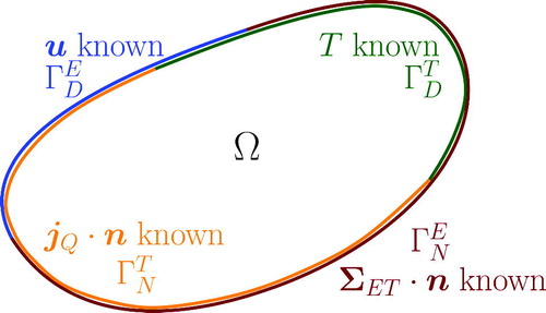
Given a partition of the boundary $\partial \Omega ={\Gamma }_D^E\cup {\Gamma }_N^E={\Gamma }_D^T\cup {\Gamma }_N^T$ for the elastic and thermal domain, the general boundary conditions read (see Figure 1) (5) $$\begin{array}{c}\text{Dirichletb}.\mathrm{c}.:\hfill \\ \text{Neumannb}.\mathrm{c}.:\hfill \end{array}\mathrm{\hspace{1em}}\mathrm{\hspace{1em}}\begin{array}{c}\mathit{u}\mathrm{ }\text{known}\mathrm{ }\text{on}\mathrm{ }{\Gamma }_D^E\times (0,+\infty ),\hfill \\ {\mathbf{\Sigma }}_{ET}·\mathit{n}\mathrm{ }\text{known}\mathrm{ }\text{on}\mathrm{ }{\Gamma }_N^E\times (0,+\infty ),\hfill \end{array}\mathrm{\hspace{1em}}\mathrm{\hspace{1em}}\begin{array}{c}T\mathrm{ }\text{known}\mathrm{ }\text{on}\mathrm{ }{\Gamma }_D^T\times (0,+\infty ),\hfill \\ {\mathit{j}}_Q·\mathit{n}\mathrm{ }\text{known}\mathrm{ }\text{on}\mathrm{ }{\Gamma }_N^T\times (0,+\infty ),\hfill \end{array}$$(5) where n is the outgoing normal vector at the boundary. Note that there are 4 different cases of boundary conditions all together, since at each point of the boundary both a vectorial b.c. on the elastic part and a scalar b.c. on the thermal part must be taken into account. In the following sections, the pHs formulation of the heat equation and elastodynamics are given. Then, an equivalent coupled system is constructed by interconnecting these two systems in a structured manner.

Figure 1. Boundary conditions for the thermoelastic problem, with 4 cases.

2.2. The heat equation as a port-Hamiltonian descriptor system

Consider the heat equation in a bounded connected set $\Omega \subset {\mathbb{R}}^d, d\in \{1,2,3\},$ describing the evolution of the temperature field $T(\mathit{x},t)$ (6) $$\rho c_{ϵ}\frac{\partial T}{\partial t}=\text{div}\mathrm{ }(k\mathrm{ }\text{grad}\mathrm{ }T)+u_T,\mathrm{\hspace{1em}}\mathrm{\hspace{1em}}\hspace{1em}\mathit{x}\in \Omega ,$$(6) where $\rho , c_{ϵ}, k$ have the same meaning as in (1)(1) $$\begin{array}{c}\rho \frac{{\partial }^2\mathit{u}}{\partial t^2}=\text{Div}({\mathbf{\Sigma }}_{ET}),\hfill \\ \rho c_{ϵ}\frac{\partial T}{\partial t}=-\text{div}({\mathit{j}}_Q)-{\mathcal{C}}_{\beta }:\frac{\partial \mathit{\epsilon }}{\partial t},\hfill \\ {\mathbf{\Sigma }}_{ET}={\mathbf{\Sigma }}_E+{\mathbf{\Sigma }}_T,\hfill \\ {\mathbf{\Sigma }}_E=\mathcal{D}(\mathit{\epsilon }),\hfill \\ {\mathbf{\Sigma }}_T=-{\mathcal{C}}_{\beta }\theta ,\mathrm{\hspace{1em}}\mathrm{\hspace{1em}}\theta :=(T-T_0)/T_0,\hfill \\ \mathit{\epsilon }=\text{Grad}\mathrm{ }(\mathit{u}),\hfill \\ {\mathit{j}}_Q=-k \text{grad}\mathrm{ }T.\hfill \end{array}$$(1) and u_T is a distributed heat source. This model can be put in pH form by means of a canonical interconnection structure. To model the Fourier law, an algebraic relationship has to be incorporated to obtain a pH system (cf. [8, Chapter 2]). Here, in the same manner, a differential-algebraic formulation is exploited.

Let T₀ be a constant reference temperature (the introduction of this variable is instrumental for coupled thermoelasticity). The functional $$H_T=\frac{1}{2}{\int }_{\Omega }\rho c_{ϵ}{T}_0{\left(\frac{T-T_0}{T_0}\right)}^2\mathrm{d}\Omega$$ has the physical dimension of an energy and represents a Lyapunov functional of this system. Even though it does not represent the internal energy, which is classically used in thermodynamics, it has some important and useful properties. Select as energy variable $${\alpha }_T:=\rho c_{ϵ}(T-T_0).$$

The corresponding co-energy is $$e_T:=\frac{\delta H_T}{\delta {\alpha }_T}=\frac{{\alpha }_T}{\rho c_{ϵ}{T}_0}=\frac{T-T_0}{T_0}=:\theta .$$

Introducing the heat flux ${\mathit{j}}_Q:=-k\mathrm{ }\text{grad}\mathrm{ }T$ as additional variable, the heat equation (6(6) $$\rho c_{ϵ}\frac{\partial T}{\partial t}=\text{div}\mathrm{ }(k\mathrm{ }\text{grad}\mathrm{ }T)+u_T,\mathrm{\hspace{1em}}\mathrm{\hspace{1em}}\hspace{1em}\mathit{x}\in \Omega ,$$(6) ) is equivalently reformulated as (7) $$\begin{array}{c}\left[\begin{array}{cc}1& 0\\ \mathit{0}& \mathit{0}\end{array}\right]\frac{\partial }{\partial t}\left(\begin{array}{c}{\alpha }_T\\ {\mathit{j}}_Q\end{array}\right)=\left[\begin{array}{cc}0& -\text{div}\\ -\text{grad}& -{(T_{0}k)}^{-1}\end{array}\right]\left(\begin{array}{c}{e}_T\\ {\mathit{j}}_Q\end{array}\right)+\left[\begin{array}{c}1\\ \mathit{0}\end{array}\right]u_T,\hfill \\ y_T=\left[\begin{array}{cc}1& \mathit{0}\end{array}\right]\left(\begin{array}{c}{e}_T\\ {\mathit{j}}_Q\end{array}\right),\hfill \end{array}$$(7) where y_T represents the distributed output, which is power-conjugated to the distributed heat source input u_T. In matrix notation, it is obtained (8) $$\begin{array}{c}{\mathcal{E}}_T{\partial }_t{\mathit{\alpha }}_T=\left({\mathcal{J}}_T-{\mathcal{R}}_T\right){\mathit{e}}_T+{\mathcal{B}}_T u_T,\hfill \\ y_T={\mathcal{B}}_T^{*} {\mathit{e}}_T\hfill \end{array}$$(8) where ${\mathit{\alpha }}_T=({\alpha }_T,{\mathit{j}}_Q),{\mathit{e}}_T=(e_T,{\mathit{j}}_Q)$ and $${\mathcal{E}}_T=\left[\begin{array}{cc}1& 0\\ \mathit{0}& \mathit{0}\end{array}\right],\hspace{1em}{\mathcal{J}}_T=\left[\begin{array}{cc}0& -\text{div}\\ -\text{grad}& \mathit{0}\end{array}\right],\hspace{1em}{\mathcal{R}}_T=\left[\begin{array}{cc}0& 0\\ \mathit{0}& {(T_{0}k)}^{-1}\end{array}\right],\hspace{1em}{\mathcal{B}}_T=\left[\begin{array}{c}1\\ \mathit{0}\end{array}\right].$$

This system is an example of pH descriptor system (cf. [21, 22] for the finite-dimensional case). The Hamiltonian reads (9) $$H_T=\frac{1}{2}{\int }_{\Omega }\frac{{\alpha }_T^2}{\rho {ϵ}_{\epsilon }{T}_0}\mathrm{d}\Omega .$$(9)

The power rate is then deduced (10) $$\begin{array}{cc}{\dot{H}}_T={\int }_{\Omega }\frac{\delta H_T}{\delta {\alpha }_T}\frac{\partial {\alpha }_T}{\partial t}\mathrm{d}\Omega \hfill & ={\int }_{\Omega }{e}_T{\partial }_t{\alpha }_T\mathrm{d}\Omega ,\hfill \\ \hfill & ={\int }_{\Omega }{\mathit{e}}_T·{\mathcal{E}}_T {\partial }_t{\mathit{\alpha }}_T\mathrm{d}\Omega ,\hfill \\ \hfill & ={\int }_{\Omega }{\mathit{e}}_T·\left\{({\mathcal{J}}_T-{\mathcal{R}}_T){\mathit{e}}_T+{\mathcal{B}}_T{u}_T\right\}\mathrm{d}\Omega ,\hfill \\ \hfill & ={\int }_{\Omega }{u}_T y_T\mathrm{d}\Omega -{\int }_{\Omega }\left(e_T\mathrm{ }\text{div}\mathrm{ }{\mathit{j}}_Q+{\mathit{j}}_Q·\mathrm{ }\text{grad}\mathrm{ }{e}_T+\frac{\left|\right|{\mathit{j}}_Q|{|}^2}{k{T}_0}\right)\mathrm{d}\Omega ,\hfill \\ \hfill & ={\int }_{\Omega }{u}_T y_T\mathrm{d}\Omega -{\int }_{\Omega }\frac{\left|\right|{\mathit{j}}_Q|{|}^2}{k{T}_0}\mathrm{d}\Omega -{\int }_{\partial \Omega }{e}_T{\mathit{j}}_Q·\mathit{n}\mathrm{d}S,\hfill \\ \hfill & \le {\int }_{\Omega }{u}_T y_T\mathrm{d}\Omega -{\int }_{\partial \Omega }{e}_T{\mathit{j}}_Q·\mathit{n}\mathrm{d}S.\hfill \end{array}$$(10)

This choice of Hamiltonian allows retrieving the classical boundary conditions (i.e. temperature, or inward heat flux) and leads to a dissipative system. Other formulations, based on the entropy or the internal energy as Hamiltonian functionals, are possible for the heat equation [23, 24]. These provide either an accrescent or a lossless system. Unfortunately these formulations are non linear and their discretization is a difficult task [25].

2.3. Port-Hamiltonian linear elastodynamics

Consider the linearized equation of elastodynamics [20, Chapter 4] (11) $$\rho \frac{{\partial }^2\mathit{u}}{\partial t^2}(\mathit{x},t)-\mathrm{ }\text{Div}\mathrm{ }(\mathcal{D}\mathrm{ }\text{Grad}\mathrm{ }\mathit{u})=\mathit{f},\mathrm{\hspace{1em}}\mathrm{\hspace{1em}}\mathit{x}\in \Omega ,$$(11) where u and $\mathcal{D}$ have the same meaning as in (1). The term f represents an external force. To derive a pH formulation, the total energy, that includes the kinetic and deformation energy, is used (12) $$H_E=\frac{1}{2}{\int }_{\Omega }\left\{\rho \left|\right|{\partial }_t\mathit{u}|{|}^2+\mathbf{\Sigma }:\mathit{\epsilon }\right\}\mathrm{d}\Omega .$$(12)

Recall that $\mathit{\epsilon }=\text{Grad}\mathrm{ }\mathit{u}$ and $\mathbf{\Sigma }=\mathcal{D}\mathit{\epsilon }.$

The energy variables are then the linear momentum and the deformation field $${\mathit{\alpha }}_v=\rho \mathit{v},\mathrm{\hspace{1em}}\mathrm{\hspace{1em}}{\mathit{A}}_{\epsilon }=\mathit{\epsilon },$$ where $\mathit{v}:={\partial }_t\mathit{u}.$ The Hamiltonian can be rewritten as a quadratic functional in the energy variables (13) $$H_E=\frac{1}{2}{\int }_{\Omega }\left\{\frac{1}{\rho }\left|\right|{\mathit{\alpha }}_v|{|}^2+(\mathcal{D}{\mathit{A}}_{\epsilon }):{\mathit{A}}_{\epsilon }\right\}\mathrm{d}\Omega .$$(13)

The co-energy variables are given by (14) $${\mathit{e}}_v:=\frac{\delta H}{\delta {\mathit{\alpha }}_v}=\mathit{v},\mathrm{\hspace{1em}}\mathrm{\hspace{1em}}{\mathit{E}}_{\epsilon }:=\frac{\delta H}{\delta {\mathit{A}}_{\epsilon }}=\mathbf{\Sigma }.$$(14)

The tensor-valued co-energy variable ${\mathit{E}}_{\epsilon }$ is obtained by taking the variational derivative with respect to a tensor (cf. [26, Chapter 3] and [5]).

The equivalent port-Hamiltonian reformulation of system (11)(11) $$\rho \frac{{\partial }^2\mathit{u}}{\partial t^2}(\mathit{x},t)-\mathrm{ }\text{Div}\mathrm{ }(\mathcal{D}\mathrm{ }\text{Grad}\mathrm{ }\mathit{u})=\mathit{f},\mathrm{\hspace{1em}}\mathrm{\hspace{1em}}\mathit{x}\in \Omega ,$$(11) is then given by (cf. [26, Chapter 3]) (15) $$\begin{array}{c}\frac{\partial }{\partial t}\left(\begin{array}{c}{\mathit{\alpha }}_v\\ {\mathit{A}}_{\epsilon }\end{array}\right)=\left[\begin{array}{cc}\mathit{0}& \text{Div}\\ \text{Grad}& \mathit{0}\end{array}\right]\left(\begin{array}{c}{\mathit{e}}_v\\ {\mathit{E}}_{\epsilon }\end{array}\right)+\left[\begin{array}{c}{\mathit{I}}_{d\times d}\\ \mathit{0}\end{array}\right]{\mathit{u}}_E,\hfill \\ {\mathit{y}}_E=\left[\begin{array}{cc}{\mathit{I}}_{d\times d}& \mathit{0}\end{array}\right]\left(\begin{array}{c}{\mathit{e}}_v\\ {\mathit{E}}_{\epsilon }\end{array}\right),\hfill \end{array}$$(15) where the distributed input ${\mathit{u}}_E:=\mathit{f}$ plays the role of the previously introduced forcing. The energy rate verifies the following (16) $$\begin{array}{cc}{\dot{H}}_E\hfill & ={\int }_{\Omega }\{{\mathit{e}}_v·{\partial }_t{\mathit{\alpha }}_v+{\mathit{E}}_{\epsilon }:{\partial }_t{\mathit{A}}_{\epsilon }\}\mathrm{d}\Omega ,\hfill \\ \hfill & ={\int }_{\Omega }{\mathit{u}}_E·{\mathit{y}}_E\mathrm{d}\Omega +{\int }_{\partial \Omega }{\mathit{e}}_v·({\mathit{E}}_{\epsilon }·\mathit{n})\mathrm{d}S.\hfill \end{array}$$(16)

2.4. Thermoelasticity as two coupled Port-Hamiltonian systems

Given the pHDAE formulation of the heat equation (7(7) $$\begin{array}{c}\left[\begin{array}{cc}1& 0\\ \mathit{0}& \mathit{0}\end{array}\right]\frac{\partial }{\partial t}\left(\begin{array}{c}{\alpha }_T\\ {\mathit{j}}_Q\end{array}\right)=\left[\begin{array}{cc}0& -\text{div}\\ -\text{grad}& -{(T_{0}k)}^{-1}\end{array}\right]\left(\begin{array}{c}{e}_T\\ {\mathit{j}}_Q\end{array}\right)+\left[\begin{array}{c}1\\ \mathit{0}\end{array}\right]u_T,\hfill \\ y_T=\left[\begin{array}{cc}1& \mathit{0}\end{array}\right]\left(\begin{array}{c}{e}_T\\ {\mathit{j}}_Q\end{array}\right),\hfill \end{array}$$(7) ) and the pH formulation of elasticity (15)(15) $$\begin{array}{c}\frac{\partial }{\partial t}\left(\begin{array}{c}{\mathit{\alpha }}_v\\ {\mathit{A}}_{\epsilon }\end{array}\right)=\left[\begin{array}{cc}\mathit{0}& \text{Div}\\ \text{Grad}& \mathit{0}\end{array}\right]\left(\begin{array}{c}{\mathit{e}}_v\\ {\mathit{E}}_{\epsilon }\end{array}\right)+\left[\begin{array}{c}{\mathit{I}}_{d\times d}\\ \mathit{0}\end{array}\right]{\mathit{u}}_E,\hfill \\ {\mathit{y}}_E=\left[\begin{array}{cc}{\mathit{I}}_{d\times d}& \mathit{0}\end{array}\right]\left(\begin{array}{c}{\mathit{e}}_v\\ {\mathit{E}}_{\epsilon }\end{array}\right),\hfill \end{array}$$(15) , linear thermoelasticity can be expressed as a coupled port-Hamiltonian system by considering the following interconnection (17) $${\mathit{u}}_E=-\text{Div}\mathrm{ }({\mathcal{C}}_{\beta } y_T),\mathrm{\hspace{1em}}\mathrm{\hspace{1em}}{u}_T=-{\mathcal{C}}_{\beta }:\text{Grad}\mathrm{ }({\mathit{y}}_E).$$(17)

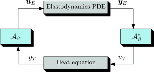
The interconnection is power preserving, since it can be compactly written as (18) $${\mathit{u}}_E={\mathcal{A}}_{\beta }(y_T),\mathrm{\hspace{1em}}\mathrm{\hspace{1em}}{u}_T=-{\mathcal{A}}_{\beta }^{*}({\mathit{y}}_E),\text{where}{\mathcal{A}}_{\beta }(·)=-\text{Div}\mathrm{ }({\mathcal{C}}_{\beta } ·),$$(18)

where ${\mathcal{A}}_{\beta }^{*}$ denotes the formal adjoint (cf. Figure 2). The assertion is justified by the following proposition.

Figure 2. Schematic interconnection block diagram for linear thermoelasticity.

Proposition 1.

Let $C_0^{\infty }(\Omega ),C_0^{\infty }(\Omega ,{\mathbb{R}}^d)$ be the space of smooth scalar functions and vector-valued functions with compact support in Ω. Given $y_T\in C_0^{\infty }(\Omega ),{\mathit{y}}_E\in C_0^{\infty }(\Omega ,{\mathbb{R}}^d)$, the coupling operator (19) $$\begin{array}{c}{\mathcal{A}}_{\beta }:C_0^{\infty }(\Omega )\to C_0^{\infty }(\Omega ,{\mathbb{R}}^d),\hfill \\ y_T\to -\text{Div}\mathrm{ }({\mathcal{C}}_{\beta }{y}_T)\hfill \end{array}$$(19) has formal adjoint (20) $$\begin{array}{c}{\mathcal{A}}_{\beta }^{*}:C_0^{\infty }(\Omega ,{\mathbb{R}}^d)\to C_0^{\infty }(\Omega )\hfill \\ {\mathit{y}}_E\to +{\mathcal{C}}_{\beta }:\mathrm{ }\text{Grad}\mathrm{ }({\mathit{y}}_E)\hfill \end{array}$$(20)

Proof.

It is necessary to show (21) $${〈{\mathit{y}}_E, {\mathcal{A}}_{\beta }{y}_T〉}_{L^2(\Omega ,{\mathbb{R}}^d)}={〈{\mathcal{A}}_{\beta }^{*}{\mathit{y}}_E, y_T〉}_{L^2(\Omega )},$$(21) where for ${\mathit{u}}_E,{\mathit{y}}_E\in C_0^{\infty }(\Omega ),u_T,y_T\in C_0^{\infty }(\Omega )$ (22) $${〈{\mathit{u}}_E, {\mathit{y}}_E〉}_{L^2(\Omega ,{\mathbb{R}}^d)}={\int }_{{\Omega }_E}{\mathit{u}}_E·{\mathit{y}}_E\mathrm{d}\Omega ,\mathrm{\hspace{1em}}\mathrm{\hspace{1em}}{〈u_T, y_T〉}_{L^2(\Omega )}={\int }_{{\Omega }_T}{u}_T{y}_T\mathrm{d}\Omega .$$(22)

By applying the integration by parts, the proof is readily obtained (23) $$\begin{array}{cc}{〈{\mathit{y}}_E, {\mathcal{A}}_{\beta }{y}_T〉}_{L^2(\Omega ,{\mathbb{R}}^d)}\hfill & =-{\int }_{\Omega }{\mathit{y}}_E·\text{Div}\mathrm{ }({\mathcal{C}}_{\beta }{y}_T)\mathrm{d}\Omega ,\hfill \\ \hfill & ={\int }_{\Omega }\mathrm{ }\text{Grad}\mathrm{ }({\mathit{y}}_E):{\mathcal{C}}_{\beta }{y}_T\mathrm{d}\Omega ,\hfill \\ \hfill & ={\int }_{\Omega }{\mathcal{A}}_{\beta }^{*}({\mathit{y}}_E)y_T\mathrm{d}\Omega ,\hfill \\ \hfill & ={〈{\mathcal{A}}_{\beta }^{*}{\mathit{y}}_E, y_T〉}_{L^2(\Omega )}.\hfill \end{array}$$(23)

If the compact support assumption is removed, it is obtained (24) $$\begin{array}{cc}{〈u_T,y_T〉}_{L^2(\Omega )}+{〈{\mathit{u}}_E,{\mathit{y}}_E〉}_{L^2(\Omega ,{\mathbb{R}}^3)}\hfill & =-{\int }_{\Omega }\left\{({\mathcal{C}}_{\beta }:\mathrm{ }\text{Grad}\mathrm{ }{\mathit{e}}_v)e_T+\text{Div}\mathrm{ }({\mathcal{C}}_{\beta }{e}_T)·{\mathit{e}}_v\right\}\mathrm{d}\Omega ,\hfill \\ \hfill & =-{\int }_{\Omega }\mathrm{ }\text{div}\mathrm{ }(e_T {\mathcal{C}}_{\beta }·{\mathit{e}}_v)\mathrm{d}\Omega ,\hfill \\ \hfill & =-{\int }_{\partial \Omega }(e_T {\mathcal{C}}_{\beta }·\mathit{n})·{\mathit{e}}_v\mathrm{d}S.\hfill \end{array}$$(24)

Using the expression of $y_T,{\mathit{y}}_E,$ considering that T₀ is constant and applying Schwarz theorem for smooth function, the inputs are equal to $${\mathit{u}}_E=\text{Div}\mathrm{ }({\mathbf{\Sigma }}_T),\mathrm{\hspace{1em}}\mathrm{\hspace{1em}}{u}_T=-{\mathcal{C}}_{\beta }:\mathrm{ }\text{Grad}\mathrm{ }(\mathit{v})=-{\mathcal{C}}_{\beta }:\frac{\partial \mathit{\epsilon }}{\partial t}.$$

The coupled thermoelastic problem can now be written as (25) $$\left[\begin{array}{cccc}\mathit{1}& \mathit{0}& \mathit{0}& \mathit{0}\\ \mathit{0}& \mathit{1}& \mathit{0}& \mathit{0}\\ 0& 0& 1& 0\\ \mathit{0}& \mathit{0}& \mathit{0}& \mathit{0}\end{array}\right]\frac{\partial }{\partial t}\left(\begin{array}{c}{\mathit{\alpha }}_v\\ {\mathit{A}}_{\epsilon }\\ {\alpha }_T\\ {\mathit{j}}_Q\end{array}\right)=\left[\begin{array}{cccc}\mathit{0}& \text{Div}\mathrm{ }& {\mathcal{A}}_{\beta }& \mathit{0}\\ \text{Grad}& \mathit{0}& \mathit{0}& \mathit{0}\\ -{\mathcal{A}}_{\beta }^{*}& 0& 0& -\text{div}\\ \mathit{0}& \mathit{0}& -\mathrm{ }\text{grad}\mathrm{ }& -{(T_{0}k)}^{-1}\end{array}\right]\left(\begin{array}{c}{\mathit{e}}_v\\ {\mathit{E}}_{\epsilon }\\ e_T\\ {\mathit{j}}_Q\end{array}\right),$$(25) with total energy given by $H=H_E+H_T.$ The power balance for each subsystem is given by (26) $${\dot{H}}_E={\int }_{\Omega }{\mathit{u}}_E·{\mathit{y}}_E\mathrm{d}\Omega +{\int }_{\partial \Omega }{\mathit{e}}_v·({\mathit{E}}_{\epsilon }·\mathit{n})\mathrm{d}S,$$(26) (27) $${\dot{H}}_T\le {\int }_{\Omega }{u}_T{y}_T\mathrm{d}\Omega -{\int }_{\partial \Omega }\theta {\mathit{j}}_Q·\mathit{n}\mathrm{d}S,$$(27)

The overall power balance is easily computed considering Eqs. (26)(26) $${\dot{H}}_E={\int }_{\Omega }{\mathit{u}}_E·{\mathit{y}}_E\mathrm{d}\Omega +{\int }_{\partial \Omega }{\mathit{e}}_v·({\mathit{E}}_{\epsilon }·\mathit{n})\mathrm{d}S,$$(26) , (27)(27) $${\dot{H}}_T\le {\int }_{\Omega }{u}_T{y}_T\mathrm{d}\Omega -{\int }_{\partial \Omega }\theta {\mathit{j}}_Q·\mathit{n}\mathrm{d}S,$$(27) and (24)(24) $$\begin{array}{cc}{〈u_T,y_T〉}_{L^2(\Omega )}+{〈{\mathit{u}}_E,{\mathit{y}}_E〉}_{L^2(\Omega ,{\mathbb{R}}^3)}\hfill & =-{\int }_{\Omega }\left\{({\mathcal{C}}_{\beta }:\mathrm{ }\text{Grad}\mathrm{ }{\mathit{e}}_v)e_T+\text{Div}\mathrm{ }({\mathcal{C}}_{\beta }{e}_T)·{\mathit{e}}_v\right\}\mathrm{d}\Omega ,\hfill \\ \hfill & =-{\int }_{\Omega }\mathrm{ }\text{div}\mathrm{ }(e_T {\mathcal{C}}_{\beta }·{\mathit{e}}_v)\mathrm{d}\Omega ,\hfill \\ \hfill & =-{\int }_{\partial \Omega }(e_T {\mathcal{C}}_{\beta }·\mathit{n})·{\mathit{e}}_v\mathrm{d}S.\hfill \end{array}$$(24) . (28) $$\begin{array}{c}\dot{H}={\dot{H}}_E+{\dot{H}}_T\le {\int }_{\partial \Omega }\left\{\left[{\mathit{E}}_{\epsilon }-e_T{\mathcal{C}}_{\beta }\right]·\mathit{n}\right\}·{\mathit{e}}_v\mathrm{d}S-{\int }_{\partial \Omega }{e}_T{\mathit{j}}_Q·\mathit{n}\mathrm{d}S.\hfill \end{array}$$(28)

This result is the same as the one stated in [18, p. 332]. From the power balance the classical boundary conditions are retrieved. This allows defining appropriate boundary operators for the thermoelastic problem (29) $${\mathit{u}}_{\partial }=\underset{{\mathcal{B}}_{\partial }}{\underbrace{\left[\begin{array}{cccc}{\mathit{\gamma }}_0^{{\Gamma }_D^E}& \mathit{0}& \mathit{0}& \mathit{0}\\ \mathit{0}& {\mathit{\gamma }}_{\perp }^{{\Gamma }_N^E}& -{\mathit{\gamma }}_{\perp }^{{\Gamma }_N^E}({\mathcal{C}}_{\beta } ·)& \mathit{0}\\ 0& 0& {\gamma }_0^{{\Gamma }_D^T}& 0\\ \mathit{0}& \mathit{0}& \mathit{0}& {\mathit{\gamma }}_{\perp }^{{\Gamma }_N^T}\end{array}\right]}}\left(\begin{array}{c}{\mathit{e}}_v\\ {\mathit{E}}_{\epsilon }\\ e_T\\ {\mathit{j}}_Q\end{array}\right),{\mathit{y}}_{\partial }=\underset{{\mathcal{C}}_{\partial }}{\underbrace{\left[\begin{array}{cccc}\mathit{0}& {\mathit{\gamma }}_{\perp }^{{\Gamma }_D^E}& -{\mathit{\gamma }}_{\perp }^{{\Gamma }_D^E}({\mathcal{C}}_{\beta } ·)& \mathit{0}\\ {\mathit{\gamma }}_0^{{\Gamma }_N^E}& \mathit{0}& \mathit{0}& \mathit{0}\\ \mathit{0}& \mathit{0}& \mathit{0}& {\mathit{\gamma }}_{\perp }^{{\Gamma }_D^T}\\ 0& 0& {\gamma }_0^{{\Gamma }_N^T}& 0\end{array}\right]}}\left(\begin{array}{c}{\mathit{e}}_v\\ {\mathit{E}}_{\epsilon }\\ e_T\\ {\mathit{j}}_Q\end{array}\right).$$(29)

The notation ${\mathit{\gamma }}_0^{{\Gamma }_{*}^{°}}$ (with $*=\{D,N\}$ and $°=\{E,T\}$) indicates the Dirichlet trace over the set ${\Gamma }_{*}^{°},$ namely ${\mathit{\gamma }}_0^{{\Gamma }_{*}^{°}}a=a{|}_{{\Gamma }_{*}^{°}},$ and ${\mathit{\gamma }}_{\perp }^{{\Gamma }_{*}^{°}}$ indicates the normal trace along ${\Gamma }_{*}^{°},$ namely ${\mathit{\gamma }}_{\perp }^{{\Gamma }_{*}^{°}}\mathit{a}=\mathit{a}·\mathit{n}{|}_{{\Gamma }_{*}^{°}}.$

System (25) together with (29) is a pH system with collocated boundary control and observation. Indeed, it shows that the classical thermoelastic problem can be modeled as two coupled subsystems, demonstrating the modularity of the pH paradigm.

Remark 1.

Notice that the boundary operators in Eq. (29)(29) $${\mathit{u}}_{\partial }=\underset{{\mathcal{B}}_{\partial }}{\underbrace{\left[\begin{array}{cccc}{\mathit{\gamma }}_0^{{\Gamma }_D^E}& \mathit{0}& \mathit{0}& \mathit{0}\\ \mathit{0}& {\mathit{\gamma }}_{\perp }^{{\Gamma }_N^E}& -{\mathit{\gamma }}_{\perp }^{{\Gamma }_N^E}({\mathcal{C}}_{\beta } ·)& \mathit{0}\\ 0& 0& {\gamma }_0^{{\Gamma }_D^T}& 0\\ \mathit{0}& \mathit{0}& \mathit{0}& {\mathit{\gamma }}_{\perp }^{{\Gamma }_N^T}\end{array}\right]}}\left(\begin{array}{c}{\mathit{e}}_v\\ {\mathit{E}}_{\epsilon }\\ e_T\\ {\mathit{j}}_Q\end{array}\right),{\mathit{y}}_{\partial }=\underset{{\mathcal{C}}_{\partial }}{\underbrace{\left[\begin{array}{cccc}\mathit{0}& {\mathit{\gamma }}_{\perp }^{{\Gamma }_D^E}& -{\mathit{\gamma }}_{\perp }^{{\Gamma }_D^E}({\mathcal{C}}_{\beta } ·)& \mathit{0}\\ {\mathit{\gamma }}_0^{{\Gamma }_N^E}& \mathit{0}& \mathit{0}& \mathit{0}\\ \mathit{0}& \mathit{0}& \mathit{0}& {\mathit{\gamma }}_{\perp }^{{\Gamma }_D^T}\\ 0& 0& {\gamma }_0^{{\Gamma }_N^T}& 0\end{array}\right]}}\left(\begin{array}{c}{\mathit{e}}_v\\ {\mathit{E}}_{\epsilon }\\ e_T\\ {\mathit{j}}_Q\end{array}\right).$$(29) contain a coupling between the thermal and mechanical variables. This is due to the fact that the coupling operator ${\mathcal{A}}_{\beta }$ is of differential nature; otherwise, the coupling would only appear in the domain, but not on the boundary.

3. Thermoelastic Port-Hamiltonian bending

In this section, the thermoelastic bending of thin beam and plate structures is described as a pH system. Starting from classical coupled thermoelastic models, suitable pH formulations are obtained. These couple a mechanical system defined on a reduced domain (uni-dimensional for beams, bi-dimensional for plates) to the thermal diffusion defined in the three-dimensional space.

Here, instead of detailing each physics (thermal and elastic) and the interconnection between the two, the pH system is derived from the coupled equations. It is shown that the final pH system possesses the same structure as Eq. (25)(25) $$\left[\begin{array}{cccc}\mathit{1}& \mathit{0}& \mathit{0}& \mathit{0}\\ \mathit{0}& \mathit{1}& \mathit{0}& \mathit{0}\\ 0& 0& 1& 0\\ \mathit{0}& \mathit{0}& \mathit{0}& \mathit{0}\end{array}\right]\frac{\partial }{\partial t}\left(\begin{array}{c}{\mathit{\alpha }}_v\\ {\mathit{A}}_{\epsilon }\\ {\alpha }_T\\ {\mathit{j}}_Q\end{array}\right)=\left[\begin{array}{cccc}\mathit{0}& \text{Div}\mathrm{ }& {\mathcal{A}}_{\beta }& \mathit{0}\\ \text{Grad}& \mathit{0}& \mathit{0}& \mathit{0}\\ -{\mathcal{A}}_{\beta }^{*}& 0& 0& -\text{div}\\ \mathit{0}& \mathit{0}& -\mathrm{ }\text{grad}\mathrm{ }& -{(T_{0}k)}^{-1}\end{array}\right]\left(\begin{array}{c}{\mathit{e}}_v\\ {\mathit{E}}_{\epsilon }\\ e_T\\ {\mathit{j}}_Q\end{array}\right),$$(25) .

3.1. Thermoelastic Euler-Bernoulli beam

The model for the linear thermoelastic vibrations of an isotropic thin rod is detailed in [27, 28]. The domain of the beam is uni-dimensional ${\Omega }_E=\{0,L\},$ while the thermal domain is three-dimensional ${\Omega }_T=\{0,L\}\times S,$ where S is the set representing the beam cross section. For simplicity, the set S is assumed to be constant along the x-axis. The ruling equations are (30) $$\begin{array}{cc}\rho A\frac{{\partial }^{2}w}{\partial t^2}\hfill & =-EI\frac{{\partial }^{4}w}{\partial x^4}-\beta E{T}_0\frac{{\partial }^2}{\partial x^2}{\int }_{S}z\theta \mathrm{d}y\mathrm{d}z,\mathrm{\hspace{1em}}\mathrm{\hspace{1em}}x\in \{0,L\}={\Omega }_E,\hfill \\ \rho c_{ϵ,B}{T}_0\frac{\partial \theta }{\partial t}\hfill & =\text{div}\mathrm{ }(k{T}_0\mathrm{ }\text{grad}\mathrm{ }\theta )+\beta T_{0}Ez\frac{{\partial }^{3}w}{\partial x^2\partial t},\mathrm{\hspace{1em}}\mathrm{\hspace{1em}}\hspace{1em}(x,y,z)\in {\Omega }_E\times S={\Omega }_T,\hfill \end{array}$$(30) where w(x, t) is the vertical displacement of the beam, $I={\int }_S{z}^2\mathrm{d}y\mathrm{d}z$ the second moment of area, E the Young modulus and A the area of the surface S. The constant $c_{ϵ,B}$ is due to the thermoelastic coupling (cf. [27, 28] for a detailed explanation). The other terms have the same meaning as in §2. The normalized temperature $\theta (x,y,z,t)$ depends on all spatial coordinates. For simplicity, the physical parameters are assumed to be constant.

The coupling operator is defined as (31) $${\mathcal{A}}_{\beta ,B}(y_T):=-\beta E{T}_0{\partial }_{xx}\left({\int }_{S}z{y}_T\mathrm{d}y\mathrm{d}z\right).$$(31)

To unveil an interconnection that is power preserving with respect to a certain function, the formal adjoint of the coupling operator is needed.

Proposition 2.

Let $C_0^{\infty }({\Omega }_T),C_0^{\infty }({\Omega }_E)$ be the space of smooth functions with compact support defined in Ω_T and Ω_E, respectively. Given $y_T\in C_0^{\infty }({\Omega }_T),y_E\in C_0^{\infty }({\Omega }_E)$ the formal adjoint of the coupling operator is (32) $${\mathcal{A}}_{\beta ,B}^{*}(y_E)=-\beta E{T}_{0}z {\partial }_{xx}{y}_E.$$(32)

Proof.

The formal adjoint is defined by the relation (33) $${〈y_E, {\mathcal{A}}_{\beta ,B}{y}_T〉}_{L^2({\Omega }_E)}={〈{\mathcal{A}}_{\beta ,B}^{*}{y}_E, y_T〉}_{L^2({\Omega }_T)},$$(33) where for $u_E,y_E\in C_0^{\infty }({\Omega }_E),u_T,y_T\in C_0^{\infty }({\Omega }_T)$ (34) $${〈u_E, y_E〉}_{L^2({\Omega }_E)}={\int }_{{\Omega }_E}{u}_E{y}_E\mathrm{d}x,\mathrm{\hspace{1em}}\mathrm{\hspace{1em}}{〈u_T, y_T〉}_{L^2({\Omega }_T)}={\int }_{{\Omega }_T}{u}_T{y}_T\mathrm{d}x\mathrm{d}y\mathrm{d}z.$$(34)

Using Def. (31)(31) $${\mathcal{A}}_{\beta ,B}(y_T):=-\beta E{T}_0{\partial }_{xx}\left({\int }_{S}z{y}_T\mathrm{d}y\mathrm{d}z\right).$$(31) and integration by parts, one finds (35) $$\begin{array}{cc}{〈y_E, {\mathcal{A}}_{\beta ,B}{y}_T〉}_{L^2({\Omega }_E)}\hfill & ={\int }_{{\Omega }_E}{y}_E{\mathcal{A}}_{\beta ,B}{y}_T\mathrm{d}x,\hfill \\ \hfill & =-{\int }_{{\Omega }_E}{y}_E\beta E{T}_0{\partial }_{xx}\left({\int }_{S}z{y}_T\mathrm{d}y\mathrm{d}z\right)\mathrm{d}x,\hfill \\ \hfill & =-{\int }_{{\Omega }_E}({\partial }_{xx}{y}_E)\beta E{T}_0\left({\int }_{S}z{y}_T\mathrm{d}y\mathrm{d}z\right)\mathrm{d}x,\hfill \end{array}$$(35)

Since ${\Omega }_T={\Omega }_E\times S$ and thanks to Fubini theorem, it is found (36) $$\begin{array}{cc}-{\int }_{{\Omega }_E}{\partial }_{xx}(y_E)\beta E{T}_0\left({\int }_{S}z y_T\mathrm{d}y\mathrm{d}z\right)\mathrm{d}x\hfill & =-{\int }_{{\Omega }_E}{\int }_S({\partial }_{xx}{y}_E)\beta E{T}_{0}z y_T\mathrm{d}x\mathrm{d}y\mathrm{d}z,\hfill \\ \hfill & =-{\int }_{{\Omega }_T}({\partial }_{xx}{y}_E)\beta E{T}_{0}z y_T\mathrm{d}x\mathrm{d}y\mathrm{d}z,\hfill \\ \hfill & ={〈{\mathcal{A}}_{\beta ,B}^{*}{y}_E, y_T〉}_{L^2({\Omega }_T)}.\hfill & \hfill \end{array}$$(36)

This concludes the proof. □

Using Eqs. (31)(31) $${\mathcal{A}}_{\beta ,B}(y_T):=-\beta E{T}_0{\partial }_{xx}\left({\int }_{S}z{y}_T\mathrm{d}y\mathrm{d}z\right).$$(31) and (32)(32) $${\mathcal{A}}_{\beta ,B}^{*}(y_E)=-\beta E{T}_{0}z {\partial }_{xx}{y}_E.$$(32) , system (30)(30) $$\begin{array}{cc}\rho A\frac{{\partial }^{2}w}{\partial t^2}\hfill & =-EI\frac{{\partial }^{4}w}{\partial x^4}-\beta E{T}_0\frac{{\partial }^2}{\partial x^2}{\int }_{S}z\theta \mathrm{d}y\mathrm{d}z,\mathrm{\hspace{1em}}\mathrm{\hspace{1em}}x\in \{0,L\}={\Omega }_E,\hfill \\ \rho c_{ϵ,B}{T}_0\frac{\partial \theta }{\partial t}\hfill & =\text{div}\mathrm{ }(k{T}_0\mathrm{ }\text{grad}\mathrm{ }\theta )+\beta T_{0}Ez\frac{{\partial }^{3}w}{\partial x^2\partial t},\mathrm{\hspace{1em}}\mathrm{\hspace{1em}}\hspace{1em}(x,y,z)\in {\Omega }_E\times S={\Omega }_T,\hfill \end{array}$$(30) is rewritten as (37) $$\begin{array}{cc}\rho A\frac{{\partial }^{2}w}{\partial t^2}\hfill & =-EI\frac{{\partial }^{4}w}{\partial x^4}+{\mathcal{A}}_{\beta ,B}\theta ,\hfill \\ \rho c_{ϵ,B}{T}_0\frac{\partial \theta }{\partial t}\hfill & =\text{div}\mathrm{ }(k{T}_0\mathrm{ }\text{grad}\mathrm{ }\theta )-{\mathcal{A}}_{\beta ,B}^{*}\frac{\partial w}{\partial t}.\hfill \end{array}$$(37)

Consider the Hamiltonian functional (38) $$H=H_E+H_T=\frac{1}{2}{\int }_{{\Omega }_E}\left\{\rho A{\left(\frac{\partial w}{\partial t}\right)}^2+EI{\left(\frac{{\partial }^{2}w}{\partial x^2}\right)}^2\right\}\mathrm{d}x+\frac{1}{2}{\int }_{{\Omega }_T}\rho c_{ϵ,B}{T}_0{\theta }^2\mathrm{d}x\mathrm{d}y\mathrm{d}z.$$(38)

The energy variables are chosen as follows (39) $${\alpha }_w=\rho A{\partial }_{t}w,\mathrm{\hspace{1em}}\mathrm{\hspace{1em}}{\alpha }_{\kappa }={\partial }_{xx}^{2}w,\mathrm{\hspace{1em}}\mathrm{\hspace{1em}}{\alpha }_T=\rho c_{ϵ,B} T_0 \theta .$$(39)

The corresponding co-energy variables read (40) $$e_w:=\frac{\delta H}{\delta {\alpha }_w}={\partial }_{t}w,\mathrm{\hspace{1em}}\mathrm{\hspace{1em}}{e}_{\kappa }:=\frac{\delta H}{\delta {\alpha }_{\kappa }}=EI{\partial }_{xx}^{2}w,\mathrm{\hspace{1em}}\mathrm{\hspace{1em}}{e}_T:=\frac{\delta H}{\delta {\alpha }_T}=\theta .$$(40)

System (37)(37) $$\begin{array}{cc}\rho A\frac{{\partial }^{2}w}{\partial t^2}\hfill & =-EI\frac{{\partial }^{4}w}{\partial x^4}+{\mathcal{A}}_{\beta ,B}\theta ,\hfill \\ \rho c_{ϵ,B}{T}_0\frac{\partial \theta }{\partial t}\hfill & =\text{div}\mathrm{ }(k{T}_0\mathrm{ }\text{grad}\mathrm{ }\theta )-{\mathcal{A}}_{\beta ,B}^{*}\frac{\partial w}{\partial t}.\hfill \end{array}$$(37) can now be rewritten as (41) $$\left[\begin{array}{cccc}1& 0& 0& 0\\ 0& 1& 0& 0\\ 0& 0& 1& 0\\ 0& 0& 0& 0\end{array}\right]\frac{\partial }{\partial t}\left(\begin{array}{c}{\alpha }_w\\ {\alpha }_{\kappa }\\ {\alpha }_T\\ {\mathit{j}}_Q\end{array}\right)=\left[\begin{array}{cccc}0& -{\partial }_{xx}^2& {\mathcal{A}}_{\beta ,B}& 0\\ {\partial }_{xx}^2& 0& 0& 0\\ -{\mathcal{A}}_{\beta ,B}^{*}& 0& 0& -\text{div}\\ 0& 0& -\mathrm{ }\text{grad}\mathrm{ }& -{(k{T}_0)}^{-1}\end{array}\right]\left(\begin{array}{c}{e}_w\\ e_{\kappa }\\ e_T\\ {\mathit{j}}_Q\end{array}\right),$$(41)

This system is the equivalent of (25)(25) $$\left[\begin{array}{cccc}\mathit{1}& \mathit{0}& \mathit{0}& \mathit{0}\\ \mathit{0}& \mathit{1}& \mathit{0}& \mathit{0}\\ 0& 0& 1& 0\\ \mathit{0}& \mathit{0}& \mathit{0}& \mathit{0}\end{array}\right]\frac{\partial }{\partial t}\left(\begin{array}{c}{\mathit{\alpha }}_v\\ {\mathit{A}}_{\epsilon }\\ {\alpha }_T\\ {\mathit{j}}_Q\end{array}\right)=\left[\begin{array}{cccc}\mathit{0}& \text{Div}\mathrm{ }& {\mathcal{A}}_{\beta }& \mathit{0}\\ \text{Grad}& \mathit{0}& \mathit{0}& \mathit{0}\\ -{\mathcal{A}}_{\beta }^{*}& 0& 0& -\text{div}\\ \mathit{0}& \mathit{0}& -\mathrm{ }\text{grad}\mathrm{ }& -{(T_{0}k)}^{-1}\end{array}\right]\left(\begin{array}{c}{\mathit{e}}_v\\ {\mathit{E}}_{\epsilon }\\ e_T\\ {\mathit{j}}_Q\end{array}\right),$$(25) for the bending of beams. Hence, following the same reasoning, it can be obtained starting from each subsystem in pH form by means of an appropriate interconnection.

3.2. Thermoelastic Kirchhoff plate

For the bending of thin plate, several models have been proposed [27, 29–31]. Here, the Chadwick model [27] is considered. The thin plate occupies the open connected set ${\Omega }_E\times \left\{-\frac{h}{2},\frac{h}{2}\right\},$ where h is the plate thickness. The system of equations describes the midplane vertical displacement and the evolution of the temperature in the 3 D domain (42) $$\begin{array}{cc}\rho h\frac{{\partial }^{2}w}{\partial t^2}\hfill & =-{\text{div}\mathrm{ }\text{Div}}_{2D}({\mathcal{D}}_b{\text{Hess}}_{2D}w)-\frac{\beta T_{0}E}{1-\nu }{\Delta }_{2D}\left({\int }_{-h/2}^{h/2}z\theta \mathrm{d}z\right),(x,y)\in {\Omega }_E,\hfill \\ \rho c_{ϵ,P}{T}_0\frac{\partial \theta }{\partial t}\hfill & ={\text{div}}_{3D}(k{T}_0{\mathrm{ }\text{grad}\mathrm{ }}_{3D}\theta )+\frac{\beta T_{0}Ez}{1-\nu }{\Delta }_{2D}\left(\frac{\partial w}{\partial t}\right),\hspace{1em}(x,y,z)\in {\Omega }_E\times \left\{-\frac{h}{2},\frac{h}{2}\right\}={\Omega }_T,\hfill \end{array}$$(42) where $w(x,y,t)$ is the vertical deflection, E is the Young modulus, ν the Poisson modulus and $c_{ϵ,P}$ a constant (depending on the heat capacity at constant strain and other coupling parameters, cf. [27]). Symbols ${\Delta }_{2D}={\partial }_{xx}^2+{\partial }_{yy}^2$ stands for the two-dimensional Laplacian. The notation Hess denotes the Hessian operator. This operator can be decomposed as $\text{Hess}=\text{Grad}°\mathrm{ }\text{grad}\mathrm{ }$ [6]. The subscript $2D, 3D$ refers to the spatial dependency of the operators. Tensor ${\mathit{D}}_b$ is the bending stiffness tensor, defined by (43) $${\mathcal{D}}_b(·):=\frac{E{h}^3}{12(1-{\nu }^2)}\left[(1-\nu )(·)+\nu \mathrm{ }\text{Tr}\mathrm{ }(·){\mathit{I}}_{2\times 2}\right].$$(43)

The coupling operator is here defined as (44) $${\mathcal{A}}_{\beta ,P}(y_T):=-\frac{\beta T_{0}E}{1-\nu }{\Delta }_{2D}\left({\int }_{-h/2}^{h/2}z{y}_T\mathrm{d}z\right).$$(44)

Analogously to the case of the Euler-Bernoulli beam, its formal adjoint is sought for.

Proposition 3.

Let $C_0^{\infty }({\Omega }_T),C_0^{\infty }({\Omega }_E)$ be the space of smooth functions with compact support defined in Ω_T and Ω_E respectively. Given $y_T\in C_0^{\infty }({\Omega }_T),y_E\in C_0^{\infty }({\Omega }_E)$ the formal adjoint of the coupling operator is (45) $${\mathcal{A}}_{\beta ,B}^{*}(y_E)=-\frac{\beta T_{0}Ez}{1-\nu }{\Delta }_{2D}{y}_E.$$(45)

Proof.

The proof is completely identical to that of Prop. 2. □

System (42)(42) $$\begin{array}{cc}\rho h\frac{{\partial }^{2}w}{\partial t^2}\hfill & =-{\text{div}\mathrm{ }\text{Div}}_{2D}({\mathcal{D}}_b{\text{Hess}}_{2D}w)-\frac{\beta T_{0}E}{1-\nu }{\Delta }_{2D}\left({\int }_{-h/2}^{h/2}z\theta \mathrm{d}z\right),(x,y)\in {\Omega }_E,\hfill \\ \rho c_{ϵ,P}{T}_0\frac{\partial \theta }{\partial t}\hfill & ={\text{div}}_{3D}(k{T}_0{\mathrm{ }\text{grad}\mathrm{ }}_{3D}\theta )+\frac{\beta T_{0}Ez}{1-\nu }{\Delta }_{2D}\left(\frac{\partial w}{\partial t}\right),\hspace{1em}(x,y,z)\in {\Omega }_E\times \left\{-\frac{h}{2},\frac{h}{2}\right\}={\Omega }_T,\hfill \end{array}$$(42) is rewritten as (46) $$\begin{array}{cc}\rho h\frac{{\partial }^{2}w}{\partial t^2}\hfill & =-{\text{div}\mathrm{ }\text{Div}}_{2D}({\mathcal{D}}_b{\mathrm{ }\text{Hess}}_{2D}w)+{\mathcal{A}}_{\beta ,P}\theta ,\hfill \\ \rho c_{ϵ,P}{T}_0\frac{\partial \theta }{\partial t}\hfill & ={\mathrm{ }\text{div}}_{3D}(k{T}_0{\mathrm{ }\text{grad}\mathrm{ }}_{3D}\theta )-{\mathcal{A}}_{\beta ,P}^{*}\left(\frac{\partial w}{\partial t}\right),\hfill \end{array}$$(46)

The Hamiltonian functional equals (47) $$\begin{array}{cc}H=H_E+H_T=\hfill & \frac{1}{2}{\int }_{{\Omega }_E}\left\{\rho h{\left(\frac{\partial w}{\partial t}\right)}^2+({\mathcal{D}}_b{\text{Hess}}_{2D}w):{\mathrm{ }\text{Hess}}_{2D}w\right\}\mathrm{d}x\mathrm{d}y\hfill \\ \hfill & +\frac{1}{2}{\int }_{{\Omega }_T}\rho c_{ϵ,P}{T}_0{\theta }^2\mathrm{d}x\mathrm{d}y\mathrm{d}z.\hfill \end{array}$$(47)

The energy and co-energy variables are (48) $$\begin{array}{c}{\alpha }_w=\rho h{\partial }_{t}w,\hfill \\ e_w={\partial }_{t}w,\hfill \end{array}\mathrm{\hspace{1em}}\mathrm{\hspace{1em}}\begin{array}{c}{\mathit{A}}_{\kappa }={\text{Hess}}_{2D}w,\hfill \\ {\mathit{E}}_{\kappa }={\mathcal{D}}_b{\mathrm{ }\text{Hess}}_{2D}w,\hfill \end{array}\mathrm{\hspace{1em}}\mathrm{\hspace{1em}}\begin{array}{c}{\alpha }_T=\rho c_{ϵ,P}{T}_0\theta ,\hfill \\ e_T=\theta .\hfill \end{array}$$(48)

System (46)(46) $$\begin{array}{cc}\rho h\frac{{\partial }^{2}w}{\partial t^2}\hfill & =-{\text{div}\mathrm{ }\text{Div}}_{2D}({\mathcal{D}}_b{\mathrm{ }\text{Hess}}_{2D}w)+{\mathcal{A}}_{\beta ,P}\theta ,\hfill \\ \rho c_{ϵ,P}{T}_0\frac{\partial \theta }{\partial t}\hfill & ={\mathrm{ }\text{div}}_{3D}(k{T}_0{\mathrm{ }\text{grad}\mathrm{ }}_{3D}\theta )-{\mathcal{A}}_{\beta ,P}^{*}\left(\frac{\partial w}{\partial t}\right),\hfill \end{array}$$(46) is rewritten as (49) $$\left[\begin{array}{cccc}1& 0& 0& 0\\ 0& \mathit{1}& 0& 0\\ 0& 0& 1& 0\\ 0& 0& 0& 0\end{array}\right]\frac{\partial }{\partial t}\left(\begin{array}{c}{\alpha }_w\\ {\mathit{A}}_{\kappa }\\ {\alpha }_T\\ {\mathit{j}}_Q\end{array}\right)=\left[\begin{array}{cccc}0& -{\text{div}\mathrm{ }\text{Div}}_{2D}& {\mathcal{A}}_{\beta ,P}& 0\\ {\text{Hess}}_{2D}& 0& 0& 0\\ -{\mathcal{A}}_{\beta ,P}^{*}& 0& 0& -{\text{div}}_{3D}\\ 0& 0& -{\mathrm{ }\text{grad}\mathrm{ }}_{3D}& -{(k{T}_0)}^{-1}\end{array}\right]\left(\begin{array}{c}{e}_w\\ {\mathit{E}}_{\kappa }\\ e_T\\ {\mathit{j}}_Q\end{array}\right),$$(49) where ${\text{div}\mathrm{ }\text{Div}}_{2D}$ and ${\text{Hess}}_{2D}$ are formally adjoint operators [6]. The final system reproduces the same structured coupling already observed for (25) and (41) before.

Remark 2.

The choice can be made to reduce the thermoelastic bending to two problems defined on the same spatial domain (cf. [16] for beams in 1D, and [15] for plates in 2D) by introducing the following approximation of the temperature field (50) $$\theta (x,y,z)={\theta }_0+z {\theta }_1,$$(50) where ${\theta }_0={\theta }_0(x),{\theta }_1={\theta }_1(x)$ for beams, and ${\theta }_0={\theta }_0(x,y),{\theta }_1={\theta }_1(x,y)$ for plates. This introduces a strong simplification, since the thermal phenomena typically occur in the whole three-dimensional space, and not only in 1D or 2D as this approach implies.

Remark 3

(Lagnese [29] and Nowacki [32] models in pH form). The models by Lagnese and Nowacki consider the thermal evolution equation in the variable $$\Theta (x,y,t)=\frac{1}{I}{\int }_{-h/2}^{h/2}z\theta (x,y,z,t)\mathrm{d}z,\mathrm{\hspace{1em}}\mathrm{\hspace{1em}}\text{where}\hspace{1em}I=\frac{h^3}{12},$$ corresponding to the first moment of the temperature. In their formulation, a linear term appears in the evolution equation for the temperature. This term arises from the second derivative with respect to z in the Laplacian $${\int }_{-h/2}^{h/2}z\frac{{\partial }^2}{\partial z^2}\theta (x,y,z,t)\mathrm{d}z=(z{\partial }_z\theta -\theta ){|}_{-h/2}^{h/2}=-\theta {|}_{-h/2}^{h/2}.$$

The term ${\partial }_z\theta {|}_{-h/2}^{h/2}$ is zero because of an assumed zero flux condition on the plate faces (cf. [31]). For the second term, Lagnese and Nowacki assume that $\theta (x,y,z,t)$ is linear in z [31]. This means that $$\theta (x,y,z,t)\approx z\Theta (x,y,t).$$

Then, it holds $$\theta (x,y,z,t){|}_{-h/2}^{h/2}=h\Theta (x,y,t),$$ so that $${\int }_{-h/2}^{h/2}z\frac{{\partial }^2}{\partial z^2}\theta (x,y,z,t)\mathrm{d}z=-h\Theta (x,y,t).$$

This obviously introduces an inconsistency, as the term in the integral should be zero. However, it allows to retrieve the damping due the term ${\partial }_{zz}\theta (x,y,z,t)$ in the reduced model. After this clarification, it is possible to state the port-Hamiltonian realization of the Nowacki and Lagnese model $$\left[\begin{array}{cccc}1& 0& 0& 0\\ 0& 1& 0& 0\\ 0& 0& 1& 0\\ 0& 0& 0& 0\end{array}\right]\frac{\partial }{\partial t}\left(\begin{array}{c}{\alpha }_w\\ {\mathit{A}}_{\kappa }\\ {\alpha }_T\\ {\mathit{j}}_Q\end{array}\right)=\left[\begin{array}{cccc}0& -{\text{div}\mathrm{ }\text{Div}}_{2D}& {\mathcal{A}}_{\beta ,P}^L& 0\\ {\text{Hess}}_{2D}& 0& 0& 0\\ -{\mathcal{A}}_{\beta ,P}^{L*}& 0& -T_{0}kh& -{\text{div}}_{2D}\\ 0& 0& -{\mathrm{ }\text{grad}\mathrm{ }}_{2D}& -{(k{T}_{0}I)}^{-1}\end{array}\right]\left(\begin{array}{c}{e}_w\\ {\mathit{E}}_{\kappa }\\ e_T\\ {\mathit{j}}_Q\end{array}\right),$$ where the underlying variables are defined as $$\begin{array}{c}{\alpha }_w=\rho h{\partial }_{t}w,\hfill \\ e_w={\partial }_{t}w,\hfill \end{array}\mathrm{\hspace{1em}}\mathrm{\hspace{1em}}\begin{array}{c}{\mathit{A}}_{\kappa }={\text{Hess}}_{2D}w,\hfill \\ {\mathit{E}}_{\kappa }={\mathcal{D}}_b{\mathrm{ }\text{Hess}}_{2D}w,\hfill \end{array}\mathrm{\hspace{1em}}\mathrm{\hspace{1em}}\begin{array}{c}{\alpha }_T=\rho c_{ϵ,P}{T}_{0}I\Theta ,\hfill \\ e_T=\Theta .\hfill \end{array}$$

Here the coupling operators ${\mathcal{A}}_{\beta ,P}^L,{\mathcal{A}}_{\beta ,P}^{L*}$ are given by $${\mathcal{A}}_{\beta ,P}^L(·)=-\frac{\beta T_{0}EI}{1-\nu }{\Delta }_{2D}(·),\mathrm{\hspace{1em}}\mathrm{\hspace{1em}}{\mathcal{A}}_{\beta ,P}^{L*}(·)=-\frac{\beta T_{0}EI}{1-\nu }{\Delta }_{2D}(·).$$

4. Mixed finite element discretization

The numerical discretization is illustrated considering the linear thermoelasticity system (25). By using the expression of the coupling operator (3), and using a pure co-energy formulation, system (25) takes the form (51) $$\left[\begin{array}{cccc}\rho & \mathit{0}& \mathit{0}& \mathit{0}\\ 0& {\mathcal{D}}^{-1}& 0& 0\\ 0& 0& \rho c_{ϵ}{T}_0& 0\\ 0& 0& 0& 0\end{array}\right]\frac{\partial }{\partial t}\left(\begin{array}{c}{\mathit{e}}_v\\ {\mathit{E}}_{\epsilon }\\ e_T\\ {\mathit{j}}_Q\end{array}\right)=\left[\begin{array}{cccc}0& \text{Div}& -C_{\beta }\mathrm{ }\text{grad}\mathrm{ }& 0\\ \text{Grad}& 0& 0& 0\\ -C_{\beta }\mathrm{ }\text{div}& 0& 0& -\text{div}\\ 0& 0& -\mathrm{ }\text{grad}\mathrm{ }& -{(T_{0}k)}^{-1}\end{array}\right]\left(\begin{array}{c}{\mathit{e}}_v\\ {\mathit{E}}_{\epsilon }\\ e_T\\ {\mathit{j}}_Q\end{array}\right),$$(51) where $C_{\beta }=T_0\beta (2\mu +3\lambda ).$ To obtain a suitable mixed formulation, the system is first put into weak form by considering the test functions ${\mathit{v}}_v\in C^{\infty }(\Omega ,{\mathbb{R}}^d),{\mathit{V}}_{\epsilon }\in C^{\infty }(\Omega ,{\mathbb{R}}_{\text{sym}}^{d\times d}),v_T\in C^{\infty }(\Omega ),{\mathit{v}}_Q\in C^{\infty }(\Omega ,{\mathbb{R}}^d):$ (52a) $${〈{\mathit{v}}_v, \rho {\partial }_t{\mathit{e}}_v〉}_{\Omega }={〈{\mathit{v}}_v, \mathrm{ }\text{Div}{\mathit{E}}_{\epsilon }〉}_{\Omega }-{〈{\mathit{v}}_v, C_{\beta }\mathrm{ }\text{grad}\mathrm{ }{e}_T〉}_{\Omega },$$(52a) (52b) $${〈{\mathit{V}}_{\epsilon }, {\mathcal{D}}^{-1}{\partial }_t{\mathit{E}}_{\epsilon }〉}_{\Omega }={〈{\mathit{V}}_{\epsilon }, \mathrm{ }\text{Grad}\mathrm{ }{\mathit{e}}_v〉}_{\Omega },$$(52b) (52c) $${〈v_T, \rho c_{ϵ}{T}_0{\partial }_t{e}_T〉}_{\Omega }=-{〈v_T, C_{\beta }\mathrm{ }\text{div}\mathrm{ }{\mathit{e}}_v〉}_{\Omega }-{〈v_T, \mathrm{ }\text{div}\mathrm{ }{\mathit{j}}_Q〉}_{\Omega },$$(52c) (52d) $$0=-{〈{\mathit{v}}_Q, \mathrm{ }\text{grad}\mathrm{ }{e}_T〉}_{\Omega }-{〈{\mathit{v}}_Q, {(T_{0}k)}^{-1}{\mathit{j}}_Q〉}_{\Omega }.$$(52d)

The notation ${〈·, ·〉}_{\Omega }$ indicates a suitable L² inner product over the domain, depending on the nature (scalar, vectorial or tensorial) of the considered variables. Two different mixed formulations can be obtained, depending on which lines undergo the integration by parts.

4.1. First mixed formulation

The first mixed formulation is obtained by integrating by parts the Div and grad operators in line (52a)(52a) $${〈{\mathit{v}}_v, \rho {\partial }_t{\mathit{e}}_v〉}_{\Omega }={〈{\mathit{v}}_v, \mathrm{ }\text{Div}{\mathit{E}}_{\epsilon }〉}_{\Omega }-{〈{\mathit{v}}_v, C_{\beta }\mathrm{ }\text{grad}\mathrm{ }{e}_T〉}_{\Omega },$$(52a) and the second div operator in (52c)(52b) $${〈{\mathit{V}}_{\epsilon }, {\mathcal{D}}^{-1}{\partial }_t{\mathit{E}}_{\epsilon }〉}_{\Omega }={〈{\mathit{V}}_{\epsilon }, \mathrm{ }\text{Grad}\mathrm{ }{\mathit{e}}_v〉}_{\Omega },$$(52b) . The following system is then obtained (53) $$\begin{array}{c}{〈{\mathit{v}}_v, \rho {\partial }_t{\mathit{e}}_v〉}_{\Omega }=-{〈\text{Grad}\mathrm{ }{\mathit{v}}_v, {\mathit{E}}_{\epsilon }〉}_{\Omega }+{〈\text{div}\mathrm{ }{\mathit{v}}_v, C_{\beta }{e}_T〉}_{\Omega }+{〈{\mathit{v}}_v, ({\mathit{E}}_{\epsilon }-{\mathcal{C}}_{\beta }{e}_T)·\mathit{n}〉}_{\partial \Omega },\hfill \\ {〈{\mathit{V}}_{\epsilon }, {\mathcal{D}}^{-1}{\partial }_t{\mathit{E}}_{\epsilon }〉}_{\Omega }={〈{\mathit{V}}_{\epsilon }, \mathrm{ }\text{Grad}\mathrm{ }{\mathit{e}}_v〉}_{\Omega },\hfill \\ {〈v_T, \rho c_{ϵ}{T}_0{\partial }_t{e}_T〉}_{\Omega }=-{〈v_T, C_{\beta }\mathrm{ }\text{div}\mathrm{ }{\mathit{e}}_v〉}_{\Omega }+{〈\text{grad}\mathrm{ }{v}_T, {\mathit{j}}_Q〉}_{\Omega }+{〈v_T, {\mathit{j}}_Q·\mathit{n}〉}_{\partial \Omega },\hfill \\ 0=-{〈{\mathit{v}}_Q, \mathrm{ }\text{grad}\mathrm{ }{e}_T〉}_{\Omega }-{〈{\mathit{v}}_Q, {(T_{0}k)}^{-1}{\mathit{j}}_Q〉}_{\Omega }.\hfill \end{array}$$(53) where ${〈·, ·〉}_{\partial \Omega }$ indicates a suitable L² inner product over the boundary. In this formulation Neumann boundary conditions are natural ones. Introducing a Galerkin approximation (54) $$\begin{array}{c}{\mathit{v}}_v=\sum _{i=1}^{n_v}{\varphi }_v^i{v}_v^i,\mathrm{\hspace{1em}}\mathrm{\hspace{1em}}{\mathit{V}}_{\epsilon }=\sum _{i=1}^{n_{\epsilon }}{\mathbf{\Phi }}_{\epsilon }^i{v}_{\epsilon }^i,\mathrm{\hspace{1em}}\mathrm{\hspace{1em}}{v}_T=\sum _{i=1}^{n_T}{\varphi }_T^i{v}_T^i,\mathrm{\hspace{1em}}\mathrm{\hspace{1em}}{\mathit{v}}_Q=\sum _{i=1}^{n_Q}{\varphi }_Q^i{v}_Q^i,\hfill \\ {\mathit{e}}_v=\sum _{i=1}^{n_v}{\varphi }_v^i{e}_v^i,\mathrm{\hspace{1em}}\mathrm{\hspace{1em}}{\mathit{E}}_{\epsilon }=\sum _{i=1}^{n_{\epsilon }}{\mathbf{\Phi }}_{\epsilon }^i{e}_{\epsilon }^i,\mathrm{\hspace{1em}}\mathrm{\hspace{1em}}{e}_T=\sum _{i=1}^{n_T}{\varphi }_T^i{e}_T^i,\mathrm{\hspace{1em}}\mathrm{\hspace{1em}}{\mathit{j}}_Q=\sum _{i=1}^{n_Q}{\varphi }_Q^i{j}_Q^i,\hfill \end{array}$$(54) the following system is obtained (55) $$\left[\begin{array}{cccc}{\mathbf{M}}_{\rho }& \mathbf{0}& \mathbf{0}& \mathbf{0}\\ \mathbf{0}& {\mathbf{M}}_{@@{\mathcal{D}}^{-1}}& \mathbf{0}& \mathbf{0}\\ \mathbf{0}& \mathbf{0}& {\mathbf{M}}_{\rho c_{ϵ}{T}_0}& \mathbf{0}\\ \mathbf{0}& \mathbf{0}& \mathbf{0}& \mathbf{0}\end{array}\right]\left(\begin{array}{c}{\stackrel{.}{\mathbf{e}}}_v\\ {\stackrel{.}{\mathbf{e}}}_{\epsilon }\\ {\stackrel{.}{\mathbf{e}}}_T\\ {\stackrel{.}{\mathbf{j}}}_Q\end{array}\right)=\left[\begin{array}{cccc}\mathbf{0}& -{\mathbf{D}}_{\text{Grad}}^{\top }& {\mathbf{D}}_{{\mathcal{A}}_{\beta }^{*}}^{\top }& \mathbf{0}\\ {\mathbf{D}}_{\text{Grad}}& \mathbf{0}& \mathbf{0}& \mathbf{0}\\ -{\mathbf{D}}_{{\mathcal{A}}_{\beta }^{*}}& \mathbf{0}& \mathbf{0}& {\mathbf{D}}_{\text{grad}}^{\top }\\ \mathbf{0}& \mathbf{0}& -{\mathbf{D}}_{\text{grad}}& -{\mathbf{R}}_Q\end{array}\right]\left(\begin{array}{c}{\mathbf{e}}_v\\ {\mathbf{e}}_{\epsilon }\\ {\mathbf{e}}_T\\ {\mathbf{j}}_Q\end{array}\right),$$(55) where, for simplicity, homogeneous boundary conditions have been assumed: $$({\mathit{E}}_{\epsilon }-{\mathcal{C}}_{\beta }{e}_T)·\mathit{n}{|}_{\partial \Omega }=\mathit{0},\mathrm{\hspace{1em}}\mathrm{\hspace{1em}}{\mathit{j}}_Q·\mathit{n}{|}_{\partial \Omega }=0.$$

The mass matrices are defined as follows $$\begin{array}{cc}{M}_{\rho }^{ij}\hfill & ={〈{\varphi }_v^i, \rho {\varphi }_v^j〉}_{\Omega },\mathrm{\hspace{1em}}\mathrm{\hspace{1em}}i,j\in \{1,n_v\},\hfill \\ M_{@@{\mathcal{D}}^{-1}}^{ij}\hfill & ={〈{\mathbf{\Phi }}_{\epsilon }^i, {\mathcal{D}}^{-1}{\mathbf{\Phi }}_{\epsilon }^j〉}_{\Omega },\mathrm{\hspace{1em}}\mathrm{\hspace{1em}}i,j\in \{1,n_{\epsilon }\},\hfill \\ M_{\rho c_{ϵ}{T}_0}^{ij}\hfill & ={〈{\varphi }_T^i, \rho c_{ϵ}{T}_0{\varphi }_v^j〉}_{\Omega },\mathrm{\hspace{1em}}\mathrm{\hspace{1em}}i,j\in \{1,n_T\},\hfill \end{array}$$

The matrices ${\mathbf{D}}_{\text{Grad}},{\mathbf{D}}_{\text{grad}}$ are given by $$\begin{array}{cc}{D}_{\text{Grad}}^{ij}\hfill & ={〈{\mathbf{\Phi }}_{\epsilon }^i, \text{Grad}\mathrm{ }{\varphi }_v^j〉}_{\Omega },\mathrm{\hspace{1em}}\mathrm{\hspace{1em}}i\in \{1,n_{\epsilon }\},\hspace{1em}j\in \{1,n_v\},\hfill \\ D_{\text{grad}}^{ij}\hfill & ={〈{\varphi }_Q^i, \text{grad}{\varphi }_T^j〉}_{\Omega },\mathrm{\hspace{1em}}\mathrm{\hspace{1em}}i\in \{1,n_Q\},\hspace{1em}j\in \{1,n_T\},\hfill \end{array}$$

The coupling matrix ${\mathbf{D}}_{{\mathcal{A}}_{\beta }^{*}}$ arises from the discretization of the coupling operator ${\mathcal{A}}_{\beta }^{*}$ $$D_{{\mathcal{A}}_{\beta }^{*}}^{ij}={〈{\varphi }_T^i, {\mathcal{A}}_{\beta }^{*}{\varphi }_v^j〉}_{\Omega }={〈{\varphi }_T^i, C_{\beta }\text{div}\mathrm{ }{\varphi }_v^j〉}_{\Omega },\mathrm{\hspace{1em}}\mathrm{\hspace{1em}}i\in \{1,n_T\},\hspace{1em}j\in \{1,n_v\}.$$

The dissipation matrix reads $$R_Q^{ij}={〈{\varphi }_Q^i, {(T_{0}k)}^{-1}{\varphi }_Q^j〉}_{\Omega },\mathrm{\hspace{1em}}\mathrm{\hspace{1em}}i,j\in \{1,n_Q\}.$$

Suitable mixed finite elements for elastodynamics and heat equations that prove compatible with this discretization are detailed in [33, 34], respectively.

4.2. Second mixed formulation

The second mixed formulation is obtained by integrating by parts the Grad operator in line (52 b), the first div operator in (52c) and the grad operator in (52d). The following system is then obtained (56) $$\begin{array}{cc}{〈{\mathit{v}}_v, \rho {\partial }_t{\mathit{e}}_v〉}_{\Omega }\hfill & ={〈{\mathit{v}}_v, \mathrm{ }\text{Div}\mathrm{ }{\mathit{E}}_{\epsilon }〉}_{\Omega }-{〈{\mathit{v}}_v, C_{\beta }\mathrm{ }\text{grad}\mathrm{ }{e}_T〉}_{\Omega },\hfill \\ {〈{\mathit{V}}_{\epsilon }, {\mathcal{D}}^{-1}{\partial }_t{\mathit{E}}_{\epsilon }〉}_{\Omega }\hfill & =-{〈\text{Div}\mathrm{ }{\mathit{V}}_{\epsilon }, {\mathit{e}}_v〉}_{\Omega }+{〈{\mathit{V}}_{\epsilon }·\mathit{n}, {\mathit{e}}_v〉}_{\partial \Omega },\hfill \\ {〈v_T, \rho c_{ϵ}{T}_0{\partial }_t{e}_T〉}_{\Omega }\hfill & ={〈\text{grad}\mathrm{ }{v}_T, C_{\beta }{\mathit{e}}_v〉}_{\Omega }-{〈v_T, \mathrm{ }\text{div}\mathrm{ }{\mathit{j}}_Q〉}_{\Omega }-{〈v_T{\mathcal{C}}_{\beta }·\mathit{n}, {\mathit{e}}_v〉}_{\partial \Omega },\hfill \\ 0\hfill & ={〈\text{div}\mathrm{ }{\mathit{v}}_Q, e_T〉}_{\Omega }-{〈{\mathit{v}}_Q, {(T_{0}k)}^{-1}{\mathit{j}}_Q〉}_{\Omega }-{〈{\mathit{v}}_Q·\mathit{n}, e_T〉}_{\partial \Omega }.\hfill \end{array}$$(56) where ${〈·, ·〉}_{\partial \Omega }$ indicates a suitable L² inner product over the boundary. In this formulation Dirichlet boundary conditions are natural: $${\mathit{e}}_v{|}_{\partial \Omega }:=\text{Velocity},\mathrm{\hspace{1em}}\mathrm{\hspace{1em}}{e}_T={\frac{T-T_0}{T_0}}_{\partial \Omega }:=\text{DimensionlessTemperature}.$$

Introducing the Galerkin approximation (54), the following system is obtained (57) $$\left[\begin{array}{cccc}{\mathbf{M}}_{\rho }& \mathbf{0}& \mathbf{0}& \mathbf{0}\\ \mathbf{0}& {\mathbf{M}}_{{\mathcal{D}}^{-1}}& \mathbf{0}& \mathbf{0}\\ \mathbf{0}& \mathbf{0}& {\mathbf{M}}_{\rho c_{ϵ}{T}_0}& \mathbf{0}\\ \mathbf{0}& \mathbf{0}& \mathbf{0}& \mathbf{0}\end{array}\right]\left(\begin{array}{c}{\stackrel{.}{\mathbf{e}}}_v\\ {\stackrel{.}{\mathbf{e}}}_{\epsilon }\\ {\stackrel{.}{\mathbf{e}}}_T\\ {\stackrel{.}{\mathbf{j}}}_Q\end{array}\right)=\left[\begin{array}{cccc}\mathbf{0}& {\mathbf{D}}_{\text{Div}}& {\mathbf{D}}_{{\mathcal{A}}_{\beta }}& \mathbf{0}\\ -{\mathbf{D}}_{\text{Div}}^{\top }& \mathbf{0}& \mathbf{0}& \mathbf{0}\\ -{\mathbf{D}}_{{\mathcal{A}}_{\beta }}^{\top }& \mathbf{0}& \mathbf{0}& -{\mathbf{D}}_{\text{div}}\\ \mathbf{0}& \mathbf{0}& {\mathbf{D}}_{\text{div}}^{\top }& -{\mathbf{R}}_Q\end{array}\right]\left(\begin{array}{c}{\mathbf{e}}_v\\ {\mathbf{e}}_{\epsilon }\\ {\mathbf{e}}_T\\ {\mathbf{j}}_Q\end{array}\right).$$(57)

The matrices ${\mathbf{D}}_{\text{Div}},{\mathbf{D}}_{\text{div}},{\mathbf{D}}_{{\mathcal{A}}_{\beta }}$ are given by (58) $$\begin{array}{cc}{D}_{\text{Div}}^{ij}\hfill & ={〈{\varphi }_v^i, \mathrm{ }\text{Div}\mathrm{ }{\mathbf{\Phi }}_{\epsilon }^j〉}_{\Omega },\mathrm{\hspace{1em}}\mathrm{\hspace{1em}}i\in \{1,n_v\},\hspace{1em}j\in \{1,n_{\epsilon }\},\hfill \\ D_{\text{div}}^{ij}\hfill & ={〈{\varphi }_T^i, \mathrm{ }\text{div}\mathrm{ }{\varphi }_Q^j〉}_{\Omega },\mathrm{\hspace{1em}}\mathrm{\hspace{1em}}i\in \{1,n_T\},\hspace{1em}j\in \{1,n_Q\},\hfill \\ D_{{\mathcal{A}}_{\beta }}^{ij}\hfill & ={〈{\varphi }_v^i, {\mathcal{A}}_{\beta }{\varphi }_T^j〉}_{\Omega }={〈{\varphi }_v^i, -C_{\beta }\mathrm{ }\text{grad}\mathrm{ }{\varphi }_T^j〉}_{\Omega },\mathrm{\hspace{1em}}\mathrm{\hspace{1em}}i\in \{1,n_v\},\hspace{1em}j\in \{1,n_T\}.\hfill \end{array}$$(58)

For this discretization, stable mixed elements for elastodynamics can be found in [35], and for the heat equation in [36].

5. Validation of the model: The Danilovskaya problem

In this section the pH discretization of the Danilovskaya problem [37] is performed. For this problem an analytical solution in the Laplace domain is available [38]. First the pH formulation is illustrated, second the discretization strategy is briefly discussed. Numerical results are then presented.

5.1. The Danilovskaya problem

The Danilovskaya problem is a one-dimensional thermoelastic model in the infinite half-space $x\ge 0.$ The initial conditions for this problem are all null. The system is excited by a sudden thermal heating at x = 0. Furthermore, the variables vanish at $\infty .$ Consequently, the following boundary conditions apply $$\begin{array}{c}T(0,t)=T_{1}H(t),\hfill \\ \underset{x\to \infty }{\lim }T(x,t)=0,\hfill \end{array}\mathrm{\hspace{1em}}\mathrm{\hspace{1em}}\begin{array}{c}{\sigma }_{ET}(0,t)=0,\hfill \\ \underset{x\to \infty }{\lim }u(x,t)=0,\hfill \end{array}$$ where H(t) is the Heaviside function. Since the effect of the elastic vibration on the thermal field is weak, a dimensionless constant $c_{\delta }$ is usually introduced to strengthen the coupling from the mechanical to the thermal domain [39]. This dimensionless constant reads (59) $$c_{\delta }=\delta \frac{\rho c_{ϵ}(2\mu +\lambda )}{{\beta }^2{(3\lambda +2\mu )}^2{T}_0},$$(59) where $\delta \in \{0,1\}$ is a variable for switching on and off the strong coupling from the mechanical to the thermal domain. The problem can now be recast as a pH system in co-energy variables (60) $$\left[\begin{array}{cccc}\rho & 0& 0& 0\\ 0& {(2\mu +\lambda )}^{-1}& 0& 0\\ 0& 0& \rho c_{ϵ}{T}_0& 0\\ 0& 0& 0& 0\end{array}\right]\frac{\partial }{\partial t}\left(\begin{array}{c}{e}_v\\ e_{\epsilon }\\ e_T\\ j_Q\end{array}\right)=\left[\begin{array}{cccc}0& {\partial }_x& {\mathcal{A}}_{\beta }& 0\\ {\partial }_x& 0& 0& 0\\ -c_{\delta }{\mathcal{A}}_{\beta }^{*}& 0& 0& -{\partial }_x\\ 0& 0& -{\partial }_x& -{(T_{0}k)}^{-1}\end{array}\right]\left(\begin{array}{c}{e}_v\\ e_{\epsilon }\\ e_T\\ j_Q\end{array}\right),$$(60) where ${\mathcal{A}}_{\beta }(·):=-{\partial }_x(C_{\beta } ·)$ (cf. Eq. (18)(18) $${\mathit{u}}_E={\mathcal{A}}_{\beta }(y_T),\mathrm{\hspace{1em}}\mathrm{\hspace{1em}}{u}_T=-{\mathcal{A}}_{\beta }^{*}({\mathit{y}}_E),\text{where}{\mathcal{A}}_{\beta }(·)=-\text{Div}\mathrm{ }({\mathcal{C}}_{\beta } ·),$$(18) ). Notice that the coupling parameter $c_{\delta }$ breaks the Hamiltonian structure. The boundary conditions in the pH variables read (61) $$e_T(0,t)=\frac{T_1-T_0}{T_0}H(t),\mathrm{\hspace{1em}}\mathrm{\hspace{1em}}(e_{\epsilon }-C_{\beta }{e}_v)(0,t)=0,$$(61) (62) $$\underset{x\to \infty }{\lim }{e}_T(x,t)=0,\underset{x\to \infty }{\lim }{e}_v(x,t)=0.$$(62)

Remark 4

(Boundary conditions for the numerical simulation). In the numerical simulation, the vanishing conditions at $\infty$ (62) are replaced by Neumann conditions at the extremity of the simulation domain $\Omega =\{0,L\}$ [39] (63) $$(e_{\epsilon }-C_{\beta }{e}_v)(L,t)=0,\mathrm{\hspace{1em}}\mathrm{\hspace{1em}}{j}_Q(L,t)=0.$$(63)

5.2. Discretization of the thermoelastic system

The first mixed formulation, detailed in §4.1, is employed here. This choice leads to the following weak form for the numerical domain $\Omega =\{0,L\}$ (64) $$\begin{array}{cc}{〈v_v, \rho {\partial }_t{e}_v〉}_{\Omega }\hfill & =-{〈{\partial }_x{v}_v, e_{\epsilon }〉}_{\Omega }+{〈{\mathcal{A}}_{\beta }^{*}{v}_v, e_T〉}_{\Omega }+{〈{\gamma }_0{v}_v, {\gamma }_n(e_{\epsilon }-C_{\beta }{e}_T)〉}_{\partial \Omega },\hfill \\ {〈v_{\epsilon }, {(2\mu +\lambda )}^{-1}{\partial }_t{e}_{\epsilon }〉}_{\Omega }\hfill & =+{〈v_{\epsilon }, {\partial }_x{e}_v〉}_{\Omega },\hfill \\ {〈v_T, \rho c_{ϵ}{T}_0{\partial }_t{e}_T〉}_{\Omega }\hfill & =-{〈v_T, c_{\delta }{\mathcal{A}}_{\beta }^{*}{e}_v〉}_{\Omega }+{〈{\partial }_x{v}_T, j_Q〉}_{\Omega }-{〈{\gamma }_0{v}_T, {\gamma }_n{j}_Q〉}_{\partial \Omega },\hfill \\ 0\hfill & =-{〈v_j, {\partial }_x{e}_T〉}_{\Omega }-{〈v_j, {(T_{0}k)}^{-1}{e}_j〉}_{\Omega },\hfill \end{array}$$(64)

where $v_v,v_{\epsilon },v_T,v_j$ are the test functions. For this discretization the boundary condition $$e_T(0,t)=\frac{T_1-T_0}{T_0}H(t),$$

is imposed strongly as an essential condition. The other boundary terms disappear because of (63)(63) $$(e_{\epsilon }-C_{\beta }{e}_v)(L,t)=0,\mathrm{\hspace{1em}}\mathrm{\hspace{1em}}{j}_Q(L,t)=0.$$(63) . The following system is obtained (65) $$\left[\begin{array}{cccc}{\mathbf{M}}_{\rho }& \mathbf{0}& \mathbf{0}& \mathbf{0}\\ \mathbf{0}& {\mathbf{M}}_{{(2\mu +\lambda )}^{-1}}& \mathbf{0}& \mathbf{0}\\ \mathbf{0}& \mathbf{0}& {\mathbf{M}}_{\rho c_{ϵ}{T}_0}& \mathbf{0}\\ \mathbf{0}& \mathbf{0}& \mathbf{0}& \mathbf{0}\end{array}\right]\left(\begin{array}{c}{\stackrel{.}{\mathbf{e}}}_v\\ {\stackrel{.}{\mathbf{e}}}_{\epsilon }\\ {\stackrel{.}{\mathbf{e}}}_T\\ {\stackrel{.}{\mathbf{e}}}_Q\end{array}\right)=\left[\begin{array}{cccc}\mathbf{0}& -{\mathbf{D}}_{\text{Grad}}^{\top }& {\mathbf{D}}_{{\mathcal{A}}_{\beta }^{*}}^{\top }& \mathbf{0}\\ {\mathbf{D}}_{\text{Grad}}& \mathbf{0}& \mathbf{0}& \mathbf{0}\\ -c_{\delta }{\mathbf{D}}_{{\mathcal{A}}_{\beta }^{*}}& \mathbf{0}& \mathbf{0}& {\mathbf{D}}_{\text{grad}}^{\top }\\ \mathbf{0}& \mathbf{0}& -{\mathbf{D}}_{\text{grad}}& -{\mathbf{R}}_Q\end{array}\right]\left(\begin{array}{c}{\mathbf{e}}_v\\ {\mathbf{e}}_{\epsilon }\\ {\mathbf{e}}_T\\ {\mathbf{e}}_Q\end{array}\right).$$(65)

5.3. Numerical results

To assess the validity of the solution, the numerical results are compared with the analytical solution in the Laplace domain. The dimensionless displacement field $\widehat{u}$ and temperature θ are introduced $$\widehat{u}=\frac{(\lambda +2\mu )}{C_x{C}_{\beta }}u,\mathrm{\hspace{1em}}\mathrm{\hspace{1em}}\widehat{T}=\frac{T-T_0}{T_0}.$$

In Table 1 the parameters for the simulation are reported. The constant C_x, C_v are the characteristic length and velocity of the problem [39]. The dimensionless constant $\widehat{L},{\widehat{t}}_{\text{end}}$ are the dimensionless length and time of the problem. The solution in the Laplace domain for the dimensionless variable is given by [38] (66) $$\begin{array}{c}\widehat{T}(s)=\frac{1}{s(C_1^2-C_2^2)}[(C_1^2-s^2)\hspace{0.17em}\text{exp}\hspace{0.17em}(-C_1\widehat{x})-(C_2^2-s^2)\hspace{0.17em}\text{exp}\hspace{0.17em}(-C_2\widehat{x})],\hfill \\ \widehat{u}(s)=-\frac{1}{s(C_1^2-C_2^2)}[C_1\hspace{0.17em}\text{exp}\hspace{0.17em}(-C_1\widehat{x})-C_2\hspace{0.17em}\text{exp}\hspace{0.17em}(-C_2\widehat{x})],\hfill \end{array}$$(66) where $\widehat{x}=x/C_x$ is the dimensionless space variable and $C_1,C_2$ are given by (67) $$\begin{array}{c}{C}_1(s)={\left[\frac{s}{2}[(1+\delta +s)+{[{(1+\delta +s)}^2-4s]}^{\frac{1}{2}}]\right]}^{\frac{1}{2}},\hfill \\ C_2(s)={\left[\frac{s}{2}[(1+\delta +s)-{[{(1+\delta +s)}^2-4s]}^{\frac{1}{2}}]\right]}^{\frac{1}{2}}.\hfill \end{array}$$(67)

Table 1. Settings and parameters for the thermoelastic problem.

Physical parameters
λ	$0.85{10}^9[\text{kg}/(\text{cm}·{\mathrm{s}}^2)]$
μ	$0.56{10}^9[\text{kg}/(\text{cm}·{\mathrm{s}}^2)]$
ρ	$7.82{10}^{-3}[\text{kg}/{\text{cm}}^3]$
$c_{ϵ}$	$4.61{10}^6[{\text{cm}}^2/(\mathrm{K}·{\mathrm{s}}^2)]$
k	$1.7{10}^3[\text{kg}·\text{cm}/(\mathrm{K}·{\mathrm{s}}^3)]$
β	$9.03{10}^{-6}[{\mathrm{K}}^{-1}]$
T0	$300[\mathrm{K}]$
L	$C_x\widehat{L}$
Cx	$k/(\rho c_{ϵ}{C}_v)$
$\widehat{L}$	10
Integrator	Crank-Nicholson
$t_{\text{end}}$	$C_v/C_x{\widehat{t}}_{\text{end}}$
Cv	$\sqrt{(\lambda +2\mu )/\rho }$
${\widehat{t}}_{\text{end}}$	4
$\Delta t$	${10}^{-3}{t}_{\text{end}}$
FE spaces	CG1 × DG0 × CG1 × DG0
N${}^{°}$ FE	200

For the semi-discretization in space, Continous Galerkin elements of order 1 (CG₁) are employed for e_v, e_T, while Discontinous Galerkin of order 0 (DG₀) are used for $e_{\epsilon },j_Q.$ This choice is in accordance with the Finite Elements constructed in [33, 34]. Given the differential-algebraic nature of the problem, an implicit method is required to perform the time integration. For this reason, the Crank-Nicholson scheme is used. The matrices are constructed using the Firedrake finite element library [40].

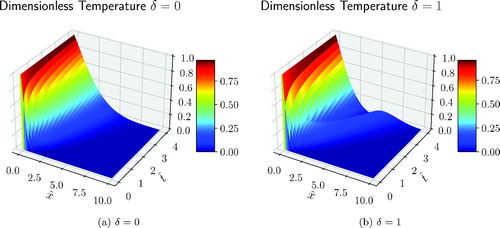
In Figure 3 the analytical and numerical displacement and temperature at $\widehat{x}=1$ are compared for weak δ = 0 and strong coupling δ = 1. The inverse of the Laplace transform is computed using the de Hoog method [41] (available through the invertlaplace function of the mpmath Python library). The displacement is retrieved from the velocity field using the trapezoidal rule. The numerical solution matches the analytical one, thus assessing the validity of the model (60) and its discretization (65). In Figures 4 and 5 the numerical solutions for the dimensionless displacement and temperature are reported for weak δ = 0 and strong coupling δ = 1.

Figure 3. Dimensionless displacement and temperature at $\widehat{x}=1.$

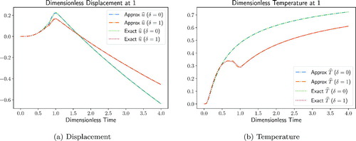
Figure 4. Displacement solution for the Danilovskaya problem.

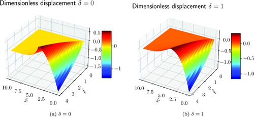
Figure 5. Temperature solution for the Danilovskaya problem.

6. Conclusion

It has been shown that classical linear thermoelastic problems are equivalent to two coupled port-Hamiltonian systems. This is especially interesting for the simulation of thermoelastic phenomena: each subsystem can be discretized separately and then coupled to the other using the discretized coupling operator. This allows to easily track how the energy flows between the two physics. Two different discretization has been proposed, depending on which kind of boundary conditions are to be weakly enforced. The best strategy is of course problem dependent. This new model of thermoelasticity may be of interest for control theorists and practitioners, given the increasing importance of port-Hamiltonian systems in control theory.

Finally, this contribution also discusses the results of discretization on a model problem only in the uni-dimensional case, where all the differential operators reduce to the same. An important point that deserves additional attention is the construction of stable mixed finite elements for the general three-dimensional problem. Reliable numerical models can then be employed for generating model-based control actions. Important future developments may include the reformulation of thermoelastic linear shells as well as non-linear thermoelasticity within the pH framework.

Acknowledgments

This work is supported by the project ANR-16-CE92-0028, entitled Interconnected Infinite-Dimensional systems for Heterogeneous Media, INFIDHEM, financed by the French National Research Agency (ANR) and the Deutsche Forschungsgemeinschaft (DFG). Further information is available at https://websites.isae-supaero.fr/infidhem/the-project.

References

- R. Rashad, F. Califano, A. J. van der Schaft, and S. Stramigioli, “Twenty years of distributed port-Hamiltonian systems: A literature review,” IMA J. Math. Control Inform., vol. 37, no. 4, pp. 1400–1422, 2020. DOI: 10.1093/imamci/dnaa018.
- M. Kurula, H. Zwart, A. J. van der Schaft, and J. Behrndt, “Dirac structures and their composition on Hilbert spaces,” J. Math. Anal. Appl., vol. 372, no. 2, pp. 402–422, 2010. DOI: 10.1016/j.jmaa.2010.07.004.
- A. Macchelli and C. Melchiorri, “Modeling and control of the Timoshenko beam. The distributed port Hamiltonian approach,” SIAM J. Control Optim., vol. 43, no. 2, pp. 743–767, 2004. DOI: 10.1137/S0363012903429530.
- S. Aoues, F. L. Cardoso-Ribeiro, D. Matignon, and D. Alazard, “Modeling and control of a rotating flexible spacecraft: A port-Hamiltonian approach,” IEEE Trans. Contr. Syst. Technol., vol. 27, no. 1, pp. 355–362, 2019. DOI: 10.1109/TCST.2017.2771244.
- A. Brugnoli, D. Alazard, V. Pommier-Budinger, and D. Matignon, “Port-Hamiltonian formulation and symplectic discretization of plate models. Part I: Mindlin model for thick plates,” Appl. Math. Modell., vol. 75, pp. 940–960, Nov. 2019. DOI: 10.1016/j.apm.2019.04.035.
- A. Brugnoli, D. Alazard, V. Pommier-Budinger, and D. Matignon, “Port-Hamiltonian formulation and symplectic discretization of plate models. Part II: Kirchhoff model for thin plates,” Appl. Math. Modell., vol. 75, 961–981, Nov. 2019. DOI: 10.1016/j.apm.2019.04.036.
- P. Kotyczka, “Structured discretization of the heat equation: Numerical properties and preservation of flatness,” in 23rd MTNS, Hong Kong, Jul. 16–20, 2018.
- P. Kotyczka, Numerical Methods for Distributed Parameter Port-Hamiltonian Systems, Technical University of Munich: TUM University Press, 2019.
- F. L. Cardoso-Ribeiro, D. Matignon, and V. Pommier-Budinger, “Port-Hamiltonian model of two-dimensional shallow water equations in moving containers,” IMA J. Math. Control Inform., vol. 37, no. 4, pp. 1348–1366, Jul. 2020. DOI: 10.1093/imamci/dnaa016.
- R. Rashad, F. Califano, F. P. Schuller, and S. Stramigioli, “Port-Hamiltonian modeling of ideal fluid flow: Part I. Foundations and kinetic energy,” Journal of Geometry and Physics, pp. 104201, 2021a. DOI: 10.1016/j.geomphys. 2021.104201.
- R. Rashad, F. Califano, F. P. Schuller, and S. Stramigioli, “Port-Hamiltonian modeling of ideal fluid flow: Part II. Compressible and incompressible flow,” Journal of Geometry and Physics, pp. 104199, 2021b. DOI: 10.1016/j.geomphys.2021.104199.
- R. Altmann and P. Schulze, “A Port-Hamiltonian formulation of the Navier–Stokes equations for reactive flows,” Syst. Control Lett., vol. 100, pp. 51–55, 2017. DOI: 10.1016/j.sysconle.2016.12.005.
- F. L. Cardoso-Ribeiro, D. Matignon, and L. Lefèvre, “A partitioned finite element method for power-preserving discretization of open systems of conservation laws,” IMA J. Math. Control Inform., vol. 12, 2020. DOI: 10.1093/imamci/dnaa038.
- R. C. Kirby and T. T. Kieu, “Symplectic-mixed finite element approximation of linear acoustic wave equations,” Numer. Math., vol. 130, no. 2, pp. 257–291, Jun. 2015. DOI: 10.1007/s00211-014-0667-4.
- G. Avalos and I. Lasiecka, “Boundary controllability of thermoelastic plates via the free boundary conditions,” SIAM J. Control Optim., vol. 38, no. 2, pp. 337–383, 2000. DOI: 10.1137/S0363012998339836.
- S. W. Hansen and B. Y. Zhang, “Boundary control of a linear thermoelastic beam,” J. Math. Anal. Appl., vol. 210, no. 1, pp. 182–205, 1997. DOI: 10.1006/jmaa.1997.5437.
- M. A. Biot, “Thermoelasticity and irreversible thermodynamics,” J. Appl. Phys., vol. 27, no. 3, pp. 240–253, 1956. DOI: 10.1063/1.1722351.
- D. E. Carlson, “Linear thermoelasticity,” in Linear Theories of Elasticity and Thermoelasticity: Linear and Nonlinear Theories of Rods, Plates, and Shells, C. Truesdell, Ed. Berlin, Heidelberg: Springer, 1973, pp. 297–345. DOI: 10.1007/978-3-662-39776-3_.2.
- R. B. Hetnarski and M. R. Eslami, Thermal Stresses: Advanced Theory and Applications, vol. 158. Springer Netherlands, Dordrecht: Springer, 2009.
- R. Abeyaratne, Lecture Notes on the Mechanics of Elastic Solids. Volume II: Continuum Mechanics, 1st ed., Cambridge, MA: American Society of Mechanical Engineers, 2012.
- C. Beattie, V. Mehrmann, H. Xu, and H. Zwart, “Linear port-Hamiltonian descriptor systems,” Math. Control Signals Syst., vol. 30, no. 4, p. 17, 2018. DOI: 10.1007/s00498-018-0223-3.
- V. Mehrmann and R. Morandin, “Structure-preserving discretization for port-Hamiltonian descriptor systems,” in 2019 IEEE 58th Conference on Decision and Control (CDC), Nice (France), 2019, pp. 6863–6868. DOI: 10.1109/CDC40024.2019.
- V. Duindam, A. Macchelli, S. Stramigioli, and H. Bruyninckx, Modeling and Control of Complex Physical Systems, Springer-Verlag Berlin Heidelberg, 2009.
- A. Serhani, G. Haine, and D. Matignon, “Anisotropic heterogeneous n-D heat equation with boundary control and observation: I. Modeling as port-Hamiltonian system,” IFAC-PapersOnLine, vol. 52, no. 7, pp. 51–56, 2019. 3rd IFAC Workshop on Thermodynamic Foundations for a Mathematical Systems Theory TFMST 2019. DOI: 10.1016/j.ifacol.2019.07.009.
- A. Serhani, G. Haine, and D. Matignon, “Anisotropic heterogeneous n-D heat equation with boundary control and observation: II. Structure-preserving discretization,” IFAC-PapersOnLine, vol. 52, no. 7, pp. 57–62, 2019. 3rd IFAC Workshop on Thermodynamic Foundations for a Mathematical Systems Theory TFMST 2019. DOI: 10.1016/j.ifacol.2019.07.010.
- A. Brugnoli, “A Port-Hamiltonian formulation of flexible structures. Modelling and structure-preserving finite element discretization,” Ph.D. thesis, Université de Toulouse, ISAE-SUPAERO, France, 2020.
- P. Chadwick, “On the propagation of thermoelastic disturbances in thin plates and rods,” J. Mech. Phys. Solids, vol. 10, no. 2, pp. 99–109, 1962. DOI: 10.1016/0022-5096(62)90013-3.
- R. Lifshitz and M. L. Roukes, “Thermoelastic damping in micro- and nanomechanical systems,” Phys. Rev. B, vol. 61, no. 8, pp. 5600–5609, 2000. DOI: 10.1103/PhysRevB.61.5600.
- J. E. Lagnese, Boundary Stabilization of Thin Plates, Society for Industrial and Applied Mathematics, University City, Philadelphia, 1989. DOI: 10.1137/1.9781611970821.
- J. G. Simmonds, “ Major simplifications in a current linear model for the motion of a thermoelastic plate,” Q. Appl. Math., vol. 57, no. 4, pp. 673–679,1999. DOI: 10.1090/qam/1724299.
- A. N. Norris, “Dynamics of thermoelastic thin plates: A comparison of four theories,” J. Therm. Stress., vol. 29, no. 2, pp. 169–195, 2006. DOI: 10.1080/01495730500257482.
- W. Nowacki, Thermoelasticity, Oxford, UK: Pergamon Press, 1962.
- G. Cohen and S. Fauqueux, “Mixed spectral finite elements for the linear elasticity system in unbounded domains,” SIAM J. Sci. Comput., vol. 26, no. 3, pp. 864–884, 2005. DOI: 10.1137/S1064827502407457.
- Z. Weng, X. Feng, and P. Huang, “A new mixed finite element method based on the Crank–Nicolson scheme for the parabolic problems,” Appl. Math. Modell., vol. 36, no. 10, pp. 5068–5079, 2012. DOI: 10.1016/j.apm.2011.12.044.
- D. Arnold and J. Lee, “Mixed methods for elastodynamics with weak symmetry,” SIAM J. Numer. Anal., vol. 52, no. 6, pp. 2743–2769, 2014. DOI: 10.1137/13095032X.
- S. Memon, N. Nataraj, and A. K. Pani, “An a posteriori error analysis of mixed finite element Galerkin approximations to second order linear parabolic problems,” SIAM J. Numer. Anal., vol. 50, no. 3, pp. 1367–1393, 2012. DOI: 10.1137/100782760.
- V. I. Danilovskaya, “Thermal stresses in an elastic half-space due to sudden heating of its boundary,” Prikladnaya Matematika i Mech., vol. 14, no. 316–318, 1950. (in Russian)
- M. Balla, “Analytical study of the thermal shock problem of a half-space with various thermoelastic models,” Acta Mech., vol. 89, no. 1–4, 73–92, Mar. 1991. DOI: 10.1007/BF01171248.
- E. Rabizadeh, A. Saboor Bagherzadeh, and T. Rabczuk, “Goal-oriented error estimation and adaptive mesh refinement in dynamic coupled thermoelasticity,” Comput. Struct., vol. 173, pp. 187–211, 2016. DOI: 10.1016/j.compstruc.2016.05.024.
- F. Rathgeber, D. A. Ham, L. Mitchell, M. Lange, F. Luporini, A. T. T. McRae, G. T. Bercea, G. R. Markall, and P. H. J. Kelly, “Firedrake: Automating the finite element method by composing abstractions,” ACM Trans. Math. Softw., vol. 43, no. 3, pp. 1–27, 2017. DOI: 10.1145/2998441.
- F. R. de Hoog, J. H. Knight, and A. N. Stokes, “An improved method for numerical inversion of Laplace transforms,” SIAM J. Sci. Stat. Comput., vol. 3, no. 3, pp. 357–366, 1982. DOI: 10.1137/0903022.