Further insights on endogenous money and the liquidity preference theory of interest

Abstract

We present a simple stock-flow consistent (SFC) model to discuss some recent claims made by Angel Asensio in a paper published in this journal regarding the relationship between endogenous money theory and the liquidity preference theory of the rate of interest. We incorporate Asensio’s assumptions as far as possible and use simulation experiments to investigate his arguments regarding the presence of a crowding-out effect, the relationship between interest rates and credit demand, and the ability of the central bank to steer interest rates through varying the stock of money. We show that in a fully-specified SFC model, some of Asensio’s conclusions are not generally valid (most importantly, the presence of a crowding-out effect is ambiguous), and that in any case, his use of a non-SFC framework leads him to leave aside important mechanisms which can contribute to a better understanding of the behavior of interest rates. More generally, this paper once more demonstrates the utility of the SFC approach in research on monetary economics.

Keywords:

• Horizontalism
• structuralism
• endogenous money
• interest rates
• stock-flow consistency

JEL-CLASSIFICATION:

• E5
• E12
• E40
• E43

In a recent paper published in this journal, Angel Asensio (2017) attempts to clarify the controversies between “horizontalists” and “structuralists” that have occurred in the field of monetary economics. In so doing, he makes his own proposal about how the money and credit markets should be formalized so as to integrate both the endogenous money view and Keynes’s liquidity preference theory of the rate of interest. Surprisingly, there is no reference in his article to the work that has been done over the last 20 years within the stock-flow consistent (SFC) approach (see Godley and Lavoie 2007; Caverzasi and Godin 2015; Nikiforos and Zezza 2017). One would have thought that this kind of work would have been highly relevant to Asensio’s effort to integrate analyses of deposits, loans and bonds, their rates of return, as well as possibly aggregate output. One purpose of the present article is to show the usefulness of the SFC approach when discussing these complex monetary and financial issues, while also taking into account what is happening in the real economy. In particular, we show that the use of a fully-specified SFC framework makes it necessary to qualify Asensio’s results even if one reproduces his assumptions as closely as possible.

The main claims made by Asensio

Angel Asensio makes three main points. The first two points will only be briefly dealt with in the current section, while the last one, with its associated claims, will be discussed in greater detail in this and the following sections.

His first point is that both the credit supply curve and the money supply curve should be drawn neither as a horizontal curve, as the “horizontalists” would put it, nor as an upward-sloping curve, as several “structuralists” would have it. Instead, as long as money is endogenous while banks provide credit on demand to creditworthy borrowers, these two curves should be negatively sloped, whereby the credit supply curve coincides with a negatively sloped credit demand curve. Perhaps these differences arise from how one perceives supply curves: either as the price that will be set at different quantities supplied, or as the quantities that will be supplied for different prices as in the standard interpretation and the one that Asensio seems to endorse. We will not discuss this any further as it appears rather idiosyncratic. Readers interested in this issue may wish to consult Sawyer (2017), who expresses his uneasiness in using the notions of a supply of money as well as that of a supply of credit. The same uneasiness about what the demand for and the supply of money deposits stand for is also briefly expressed in Lavoie (2017, 356).

The second point, made in a number of places in Asensio (2017), is that post Keynesians engaged in the horizontalist-structuralist debate have in general suffered from a confusion between flows and stocks. For instance, Asensio (2017, 329) writes that “indeed, ‘horizontalist’ and ‘structuralist’ models used to derive the money supply from the deposits resulting from the current flows of credit (less repayments) while the total money supply at a point in time should be derived from the total stock of loans outstanding (past and present) and from the central bank market interventions.” Asensio devotes a whole appendix to show that Palley (2013), who is closest to his analysis, is subject to this critique. Asensio distinguishes what he calls the “credit supply”, which is a flow, and the “total credit supply,” which is a stock; the same distinction is made with the money supply (a flow) and the total money supply (a stock): “The total demand for money at a point in time (stock) therefore is a broader notion compared with the demand for deposits resulting from the demand for credit at that time (flow)” (Asensio 2017, 335). Besides Palley, Fontana and Setterfield (2009) as well as Howells (2009) are accused of this confusion, as is Lavoie (2014, 251). Other authors may have been sloppy at times in this regard, but given that Palley was a student of James Tobin while Lavoie was the coauthor of Wynne Godley, the accusation that Palley and Lavoie are the culprits of such a slipup appears to be rather surprising since Tobin and Godley are considered to be the founders of the SFC approach, one purpose of which is precisely to avoid confusion between stocks and flows. Asensio’s claim is particularly curious in light of the fact that issues related to endogenous money theory have already been assessed in SFC frameworks (Godley 1999; Lavoie and Godley, 2001-02; Lavoie 2017) in which stock-flow errors would become immediately obvious.

As his third main point, Asensio rejects a standard assumption in post-Keynesian economics, that is, the assumption that the lending rate is equal to some base rate (e.g., the target overnight rate set by the central bank—the target federal funds rate in the United States, the main refinancing rate in the Eurozone) plus some exogenous markup. Although there is ample evidence that the conventional prime lending rate is exactly set in this way in the United States, this indeed may not be the case of lending rates applied to nonprime borrowers. Asensio argues that full accommodation of the demand for loans by creditworthy borrowers does not imply an exogenous interest rate. For Asensio (2017, 336), and this is related to his first point, “insofar as the loan supply and creditworthy demand are equal by definition, the rate of interest on loans cannot be determined by any intersection of the supply and demand for loans.” He argues that the rate of interest on bank loans ought to be competitive with the interest rates charged on financial markets, which Asensio calls the “market interest rate” or the “money market interest rate”: “The rate of interest on loans and the money market interest rate can hardly differ from one another” (ibid.).¹ In more practical terms, this market interest rate is the rate of interest on corporate paper when speaking of the short term, or the interest rate on corporate bonds when dealing with the long term.

In his effort to integrate the theory of endogenous money and Keynes’s liquidity preference theory, Asensio argues that the interest rate charged to borrowers, that is, the interest rate paid by a borrower when getting funds from a bank or from the financial markets, is equal to the central bank refinancing rate plus an endogenous markup which depends on the conditions in the market for money or liquidity (ibid., 337, 340). In a nutshell, Asensio’s central point is that “the markup reflected in the spread between the central bank refinancing interest rate and the market interest rate is endogenously determined by the total demand and supply of money, given the central bank refinancing rate” (ibid., 330).

Asensio claims that three broad consequences follow from this analysis. Firstly, an increase in liquidity preference, that is, a desire to hold more money and fewer other financial assets, will lead to an increase in market rates and hence in lending rates. Secondly, an increase in the supply of money associated with open-market operations ought to lead to a decrease in the market rate of interest and hence in the rate of interest on loans. “Central banks have the power to increase the total quantity of money much beyond the credit money by buying public and private debts in the markets” (ibid., 239). However, in a long aside, Asensio points out that market interest rates may not move after all and that such open market operations may fail to achieve the decrease in market rates, if economic agents hold firm to their belief in the existence of a conventional market interest rate, as Keynes (1936, 203–4) would have it (Asensio 2017, 340). The interest rate would only decrease temporarily, as agents would sell financial assets in an attempt to become more liquid and thereby drive the rate back up.

Finally, following up on his analysis, Asensio computes the equilibrium market rate of interest of his model, and shows that within his model a higher level of economic activity must be associated with a higher rate of interest (ibid., 343), thus recovering the standard crowding-out effect which Asensio associates with Keynes and which can be found in the standard IS/LM model. The main reason for this, from Asensio’s standpoint, is that the increase in economic activity leads to an increase in the transaction demand for money, which will not be fulfilled at a given rate of interest because this additional demand for money will go beyond the flow of money being endogenously created by the additional flow of credit.

In what follows, in part as a response to the critique that post-Keynesians are confusing stocks and flows, and also because we find interesting his idea that lending rates set by banks could be influenced by market rates, we wish to formalize Asensio’s theoretical apparatus within a SFC model. In particular, to illustrate the usefulness and clarity of this approach, we build a fairly simple SFC model with five sectors—households, firms, banks, the government, and the central bank—with five interest rates: the rate on bank deposits, the rate on bank loans, the rate on commercial paper, the rate on short-term securities issued by the government (treasury bills), and the rate paid on bank reserves at the central bank, which is assumed to be the policy rate set by the central bank. We refer to short-term securities, because, for simplification, our model will not deal with changes in asset prices, which makes more sense in the case of short-term financial assets.

Model structure

The structure of the model is relatively simple and is summarized in Tables 1 (the balance sheet matrix) and 2 (the transactions flow matrix) below.

Table 1. Balance sheet matrix.

Households		Firms	Banks	Government	Central Bank	Σ
Bank deposits	+M		−M			0
Reserves			+H		−H	0
Commercial paper	+CP	−CP				0
Bank loans		−L	+L			0
Treasury bills	+GBh			−GB	+GBcb	0
Inventories		+INV				+INV
Σ	Vh	Vf	Vb	Vg	0	+INV

Households hold bank deposits $M$, commercial paper $CP$ and treasury bills $GB$ as their assets. They receive wage income $WB$, distributed profits $F$ from both firms and banks, as well as interest payments on all their assets whilst their only expenditures are on consumption $C$. Firms hold a stock of inventories $INV$ which is financed by a combination of bank loans $L$ and commercial paper (sold to households). They receive revenue from consumption expenditure and government spending $G$, they adjust their inventory stocks, and pay taxes $T$, wages, interest and distribute profits. Banks’ assets are their loans to firms and their reserves $H$ held at the central bank, whereas their only liabilities are households’ deposits. They receive interest on loans and reserves, pay interest on deposits, and distribute their profits to households. The government collects revenue in the form of tax payments as well as central bank profits $F_{cb}$. Its expenditures consist of government spending and interest payments on bills. Deficits are financed using treasury bills. The central bank holds a fraction of treasury bills, whereas its liabilities consist of a stock of reserves of equivalent size.

The role of the buffer stock variable, which is important in ensuring the stock-flow consistency of the model, is played by $M$ for households, by $L$ for firms, by $GB$ for the government (with the central bank acting as a lender of last resort purchasing any residual amount of $GB$ not demanded by households) and by $H$ for the central bank while the banks’ balance sheet identity is implied by those of the other sectors.

Behavioral equations

In this section, we discuss the key behavioral assumptions of the model (many of which are standard in the SFC literature; see Godley and Lavoie (2007)). A full list of model equations along with the parameter and initial values used is provided in the appendix.

Firms

Firms are assumed to formulate a real inventory target based on the expected real value of sales, given by $in{v}^t={\gamma }_{inv}\mathrm{ }{s}^e$, where ${\gamma }_{inv}$ is an inverse function of the average interest rate on commercial paper and bank loans (which are used to finance inventory stocks): (1) $$\begin{array}{c}{\gamma }_{inv}={\gamma }_1-{\gamma }_{2\mathrm{ }}{r}^{av}.\end{array}$$(1)

In every period, they produce output equal to expected sales plus a fraction of the deviation of inventories from target: (2) $$\begin{array}{c}y=s^e+\psi \left(in{v}^t-in{v}_{-1}\right).\end{array}$$(2)

Firms apply a simple markup pricing formula over a constant (exogenous) unit cost, meaning that output price and the distribution of income are exogenous and constant. We assume that at any given time, firms wish to finance changes in the stock of inventories by a combination of bank loans and commercial paper; in particular we assume that a fraction ${\chi }_{cp}$ of any change in inventories is financed through commercial paper, where this fraction is given by (3) $$\begin{array}{c}{\chi }_{cp}=\left\{\begin{array}{cc}{\mathrm{\chi }}_1+{\chi }_2\left(r_{l,-1}-r_{cp,-1}\right),& \mathrm{i}\mathrm{f} \Delta INV\ge 0\\ {\chi }_1-{\chi }_2\left(r_{l,-1}-r_{cp,-1}\right),& \mathrm{i}\mathrm{f} \Delta INV<0.\end{array}\right.\end{array}$$(3)

This piecewise-linear function implies that whenever the interest rate on loans is higher than that on commercial paper, a larger fraction of increases in inventories are financed using commercial paper. Conversely, when the change in inventories is negative, firms pay off a larger fraction of those liabilities on which a higher rate of interest must be paid.² The change in the quantity of commercial paper is consequently given by (4) $$\begin{array}{c}\Delta CP={\chi }_{cp} \Delta INV,\end{array}$$(4) with the residual amount of credit demand determining the change in loans. Thus, loan demand is assumed to be fully accommodated by banks, in line with what is assumed by Asensio (2017), as we do not consider issues of creditworthiness here. Hence, in line with the arguments of Asensio (2017), firms have multiple sources of credit, and bank loans compete with commercial paper. As an aside, it should be pointed out that commercial paper cannot fully replace bank loans at the macroeconomic level since only the latter imply a creation of means of payment. An increase in inventories financed by bank loans leads to an increase in the money supply (in the first instance held by firms, consequently distributed in the form of wage payments); by contrast, an increase in inventories financed by commercial paper leads only to a redistribution of existing means of payment from households to firms as households exchange deposits for commercial paper. Moreover, note that the structure of our model implies that there is certainly no confusion between stocks and flows. There is a well-defined stock of money, $M$, as well as a stock of reserves, $H$, both of which are distinct from the changes in the respective stocks, $\Delta M$ and $\Delta H$, and the same is true for the stock of commercial paper, $CP$, and its change, $\Delta CP$, as well as the stock of bank credit, $L$, and its change, $\Delta L$, as is clarified by the balance sheet and transactions flow matrices (Tables 1 and 2).

Table 2. Transactions flow matrix.

Households		Firms Current	Capital	Banks	Government	Central Bank	Σ
Consumption	−C	+C					0
Inventory Investment		+ΔINV	−ΔINV				0
Government Spending		+G			−G		0
Taxes		−T			+T		0
Wages	+WB	−WB					0
Distr. firm profit	+Ff	−Ff					0
Distr. bank profit	+Fb			−Fb			0
Distr. CB profit					+Fcb	−Fcb	0
Interest on com. paper	+rcp,−1 CP−1	−rcp,−1 CP−1					0
Interest on loans		−rl,−1 L−1		+rl,−1 L−1			0
Interest on bills	+rgb,−1 GBh,−1				−rgb,−1 GB−1	+rgb,−1 GBcb,−1	0
Interest on deposits	+rm,−1 M−1			−rm,−1 M−1			0
Interest on reserves				+rh H−1		−rh H−1	0
(Saving)	(savh)	(0)		(0)	(savg )	(0)	0
Δ Deposits	−ΔM			+ΔM			0
Δ Com. paper	−ΔCP		+ΔCP				0
Δ Loans			+ΔL	−ΔL			0
Δ Bills	−ΔGBh				+ΔGB	−ΔGBcb	0
Δ Reserves				−ΔH		+ΔH	0
Σ	0	0	0	0	0	0	0

Households

Whilst the supply of commercial paper is determined within the firm sector, we must also formulate a demand side for it. Regarding the asset allocation of households, we assume that they formulate a demand for treasury bills based on a standard Tobinesque portfolio equation: (5) $$\begin{array}{c}G{B}_h=\left({\lambda }_{20}-{\lambda }_{21}\mathrm{ }{r}_{cp}+{\lambda }_{22}\mathrm{ }{r}_{gb}-{\lambda }_{23}\mathrm{ }{r}_m\right)V_{h,-1}-{\lambda }_{24}Y{D}^e.\end{array}$$(5)

Similarly, we posit a portfolio equation for commercial paper, but as the supply of commercial paper is already determined by the financing needs of firms, we instead solve this equation for the interest rate on commercial paper, or more specifically the spread $\epsilon$ between the interest rate on commercial paper $r_{cp}$ and the central bank target rate $r_h$. Doing so yields the following equation: (6) $$\begin{array}{c}\epsilon =\frac{CP+\left({\lambda }_{13}\mathrm{ }{r}_m+{\lambda }_{12}\mathrm{ }{r}_{gb}-{\lambda }_{10}-{\lambda }_{11}\mathrm{ }{r}_h\right)V_{h,-1}+{\lambda }_{14}Y{D}^e}{{\lambda }_{11}{V}_{h,-1}}.\end{array}$$(6)

The rate of interest on commercial paper is thus given by $r_{cp}=r_h+\epsilon$, where the markup or spread $\epsilon$ is an endogenous variable which adjusts to clear the market for commercial paper. We believe that this is exactly what Asensio (2017) has in mind when he says that the market interest rate is equal to the central bank refinancing rate plus an endogenous markup.³ Households’ asset allocation is completed by the assumption that their deposit holdings act as a residual (as one portfolio item necessarily must in this approach).

The remaining household behaviors are standard. We assume that consumption depends both on expected disposable income and household wealth (7) $$\begin{array}{c}C={\alpha }_{1}Y{D}^e+{\alpha }_2{V}_{h,-1},\end{array}$$(7) which conveniently allows us to solve for the implied stationary-state level of household wealth as a function of stationary-state consumption (which itself will turn out to be a function of exogenous government spending): (8) $$\begin{array}{c}{\mathit{V}}_h=\frac{\left(1-{\alpha }_1\right)C}{{\alpha }_2}.\end{array}$$(8)

Banks and the Central bank

In keeping with the arguments advanced by Asensio (2017) as well as Palley (2013, 207), banks are assumed to react to developments in financial markets by adjusting the loan rate $r_l$ to keep it in line with the rate on commercial paper: (9) $$\begin{array}{c}\Delta r_l=\psi \left(r_{cp,-1}\hspace{0.17em}-\hspace{0.17em}{r}_{\mathrm{l},-1}\right). \end{array}$$(9)

At the same time, banks maintain a constant spread between the loan rate and the deposit rate $r_m$, so as to make profits: (10) $$\begin{array}{c}{r}_m=r_l\hspace{0.17em}-\hspace{0.17em}\omega .\end{array}$$(10)

The banking sector is as simple as it can be. In particular banks do not hold any treasury bills and hence are not attempting to satisfy some liquidity ratio, such as the ratio of safe assets (treasury bills) to loans. In Asensio’s paper, the presence of banks is only implicit and their behavior is not described, with the exception of the adjustment of the loan rate to what he calls the “money market interest rate.”

As for the central bank, we assume that it is the residual purchaser on the market for treasury bills. This implies that the central bank has in mind a rate of interest on these bills and buys any residual amount of treasury bills left over by the household sector when the latter makes its portfolio decisions based on this treasury bill rate and the interest rates on their other two assets. In the calibration presented here, we assume that the treasury bill rate targeted by the central bank is equal to its policy rate, that is, the rate of interest paid on reserves, meaning that $r_{gb}=r_h$ so that the central bank pays exactly as much interest on reserves as it receives from bills. This means that central bank profit, $F_{cb}$ will be nil throughout and could in principle be eliminated from the tables and the equations. This is done merely for simplicity; we could just as well have supposed that the treasury bill rate targeted by the central bank is equal to its policy rate plus some exogenous markup so as to generate profits.

Government

The government undertakes an exogenous amount of government expenditure each period and collects taxes on nominal sales according to (11) $$\begin{array}{c}T=\frac{\tau }{\left(1+\tau \right)} S.\end{array}$$(11)

Together with interest payments on treasury bills at the rate $r_{gb}$ and transfers from the central bank this gives rise to an equation for the government balance: (12) $$\begin{array}{c}sa{v}_g=T\hspace{0.17em}-\hspace{0.17em}G\hspace{0.17em}-\hspace{0.17em}{r}_{gb}G{B}_{-1}+F_{cb},\end{array}$$(12)

In the stationary state, we have $sa{v}_g=0$, and we can use the above equation along with the one determining tax payments to write (13) $$\begin{array}{c}Y=\frac{\left(G+r_{gb}GB\right)\left(1+\tau \right)}{\tau },\end{array}$$(13) and (14) $$\begin{array}{c}C=Y\hspace{0.17em}-\hspace{0.17em}G=\frac{\left(G+r_{gb}\mathrm{ }GB\right)\left(1+\tau \right)}{\tau }-G\left(=YD\right).\end{array}$$(14)

These stationary-state relationships will be useful in interpreting simulation outputs.

Simulation experiments⁴

We calibrate the model to a stationary state using the initialization and parameter values detailed in the appendix. To discuss the arguments advanced by Asensio (2017), we carry out four main experiments, namely a permanent change in exogenous government spending, a permanent change in the desired inventory-to-sales ratio, a decrease in households’ demand for commercial paper (associated with an equal increase in the demand for bank deposits), and an exogenous purchase of treasury bills by the central bank aimed at increasing the stock of money in the economy. According to Asensio’s arguments, the first three experiments should be expected to lead to an increase in the endogenous interest rates ($r_l$, $r_{cp}$, and $r_m$) whereas the fourth one should lead to a decrease. Finally, we carry out a fifth experiment investigating the relationship between the central bank’s target rate and the endogenous interest rates. This is not directly related to the claims made by Asensio (2017) but gives rise to a result which may be of interest in the context of this debate.

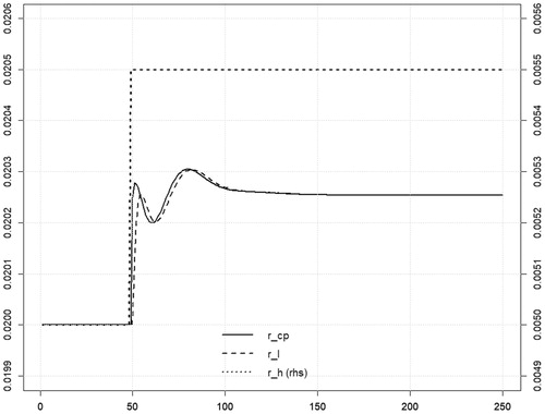
The purpose of the first experiment (an increase in government expenditure) is twofold. Firstly, as shown in Equation 13(13) $$\begin{array}{c}Y=\frac{\left(G+r_{gb}GB\right)\left(1+\tau \right)}{\tau },\end{array}$$(13) , $G$ is a primary determinant of the stationary-state level of income and hence sales, meaning that an increase in $G$ should also, indirectly, lead to an increase in credit demand (due to higher desired inventory stocks). Secondly this experiment can be used to examine Asensio’s claim that under his assumptions there exists a crowding-out effect, unless the central bank intervenes by lowering its target rate to prevent such an outcome. Figure 1 summarizes the effect of a permanent increase in exogenous government expenditure.

Figure 1. Effect of an increase in government expenditure.

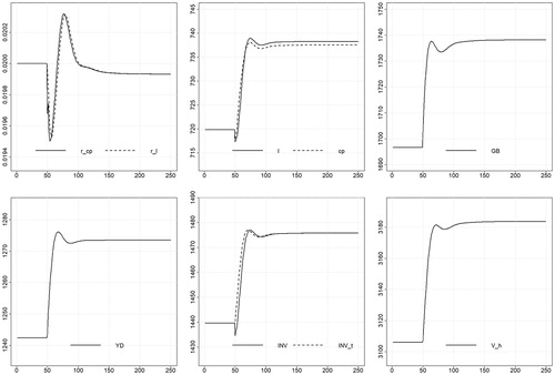
As expected, this increases both income and household wealth and leads to higher target and actual inventory stocks and consequently to an increased demand for loans and issuance of commercial paper. Curiously, however, the figure reveals that in the new stationary state, the interest rates on commercial paper and bank loans are lower (if only by very little) than in the previous one, which is the exact opposite of what would be expected based on Asensio’s arguments. Put very simply this result is because the increase in government expenditure, and consequently in income and sales, increases not only the issuance of commercial paper, but also the demand for these assets, because with a higher level of wealth (a direct consequence of higher government expenditure), households are willing to hold a greater quantity of all assets. The dynamic adjustment shows that at different points in time, different effects dominate, making the commercial paper rate at first lower and then higher than its initial value, before it eventually settles to a new lower stationary-state value. Similar simulation results—a temporary fall in interest rates followed by a return to the initial rate near the stationary state—were obtained by Lavoie (2017, 370–71), based on the model of Godley (1999) where banks have a target liquidity ratio and hence where the loan and deposit interest rates are endogenous, leading to the conclusion that one could obtain “a downward-sloping LM curve.”⁵ Palley (2017, 105) also arrives at this ambiguous result, based on his analytical model, arguing that “the LM curve in an endogenous money [sic] is not horizontal as often claimed and that the LM curve can be positively or negatively sloped depending on the relative income elasticities of loan and money demand”.

The bottom line of this first experiment is that in our model, the assumptions derived from Asensio (2017) do not necessarily imply the presence of a crowding-out effect. In the example shown here, we in fact obtain the opposite result, that is, stationary-state endogenous interest rates which are slightly lower than their previous levels. The first section of the appendix presents some simple analytical results showing that the presence or absence of a crowding-out effect is ambiguous and dependent on parameter values. Indeed, robustness checks carried out on the first experiment show that while our result is qualitatively robust to changes in most parameter values (including all reasonable variations in the portfolio parameters), higher values of the consumption propensities (implying lower stationary-state household wealth) may lead to an increase in the endogenous interest rates, while lower values lead to a stronger decrease. This is in line with the analytical results presented in the first section of the appendix. In addition, our result is sensitive to the magnitude of $\psi$, the adaptation parameter used in forming expectations. A lower value of $\psi$, implying a longer adaptation-period following a shock, may reverse our simulation result, leading to an increase in the endogenous interest rates, whereas a faster adaptation reinforces our result. Further experiments show that the crucial difference arises from the speed at which expected household disposable income adapts to its actual realized values. This finding may not seem straightforward but it underlines the main point of the analytical appendix, namely that the sign of the change in the endogenous interest rates is ambiguous and depends on the relative dynamic adjustment paths of various stock and flow variables, which obviously depend on the length of the adjustment to the new stationary state.

Consider next the effect of a direct increase in credit demand, implemented via an increase in ${\gamma }_1$ and hence the target inventory-to-sales ratio for any given average interest rate, summarized in Figure 2. It can be seen that this experiment leads to an immediate and permanent increase in the endogenous interest rates but produces only a transitory positive effect on output and income since these only increase whilst inventories adjust to their new target level. Curiously, however, we also observe that the new stationary-state levels of disposable income and household wealth are slightly lower than previously. The reason for this is that the stationary-state $Y$, $YD$ and $V_h$ are all increasing with the quantity of treasury bills (see also the further discussion provided in the first section of the appendix), due to the interest income accruing to bill holders, and that, as shown in Figure 2, an increase in target inventories leads to a decrease in the stationary-state quantity of treasury bills due to the transitory boom caused by increased inventory accumulation.⁶ The result of this second experiment is hence perfectly consistent with the result of the first, namely that the movements of the endogenous interest rates will in essence depend on the relative movements of demand for non-bank credit by firms and the supply of such credit by households.

Figure 2. Effect of an increase in the target inventory-to-sales ratio.

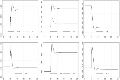
In the new stationary state, we have, because of the increased target inventory-to-sales ratio, a permanently higher demand for credit whilst the supply of non-bank credit, due to the reduction in household wealth, is smaller than in the initial stationary state. The first section of the appendix provides some further interpretation of this result, which is robust to perturbations in the values of all parameters. The crucial point to take away from the first two experiments is hence that the response of the endogenous interest rates to exogenous “shocks” depends strongly on whether and how these affect the stationary-state values of both stocks and flows in the model, leading to conclusions which are much less clear-cut than those derived from Asensio’s framework which ignores such considerations.

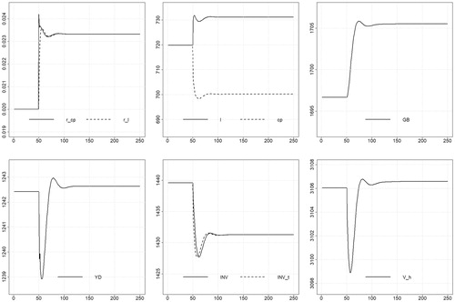
Another way to understand this result can be obtained if, instead of increasing the demand for non-bank credit by increasing the target sales-to-inventory ratio, we effectively reduce the supply of these funds by reducing the ${\lambda }_{10}$ parameter in the households’ portfolio choice equation, whilst implicitly increasing the demand for bank deposits for any given structure of interest rates. The result of this experiment is shown in Figure 3. The decreased demand for commercial paper on the part of households leads to an immediate increase in $r_{cp}$, raising $r^{av}$ and hence reducing the target sales-to-inventory ratio, which also leads to a transitory decrease in output and household wealth. Firms react to the decreased supply of nonbank credit partly by increasing their borrowing from banks and partly by reducing their overall borrowing in line with the lower target inventory stock. For the reasons already outlined above, the new stationary-state levels of government debt, of household wealth and of disposable income are marginally higher than the previous ones, but the increase in household wealth is so small that the new stationary-state supply of commercial paper remains below its previous level, meaning that the change in the endogenous interest rates is positive. This result is robust to changes in most parameter values but as with the first experiment, and for the same reason, the change in the endogenous interest rates depends crucially on the values of the consumption propensities, whereby lower values than those assumed in our baseline may lead to a decrease in the endogenous interest rates.

Figure 3. Effect of a decrease in the demand for commercial paper.

For the fourth experiment, we simply impose that at a certain point in the simulation, the central bank purchases a given amount of treasury bills from households and continues to hold these until the end of the simulation, with the aim of increasing the stock of money in the system.⁷ This is done to evaluate Asensio’s claim that the central bank can control the stock of money and thereby influence the rate of interest.

What happens in practical terms is that the central bank pays for the acquired treasury bills by transferring funds into the clearing and settlement system. As a result, households acquire bank deposits whereas the banks acquire reserves at the central bank. As three assets are involved (treasury bills, bank deposits and reserves), six of the components of the balance sheet matrix of Table 1 must change. The results of this experiment are shown in Figure 4.

Figure 4. Effect of an exogenous increase in central bank treasury bill holdings.

It can be seen that although the central bank is successful in increasing both the monetary base (reserves) and the stock of money through its intervention, this has no effect on the endogenous interest rates (or indeed any other model variable). The reason for this is simple, namely that making households exchange a part of their holdings of treasury bills for bank deposits does not by itself affect their portfolio preference for commercial paper (which is the primary driver of the endogenous interest rates). That is, unless we assume that, in response to the exogenous change in their portfolio holdings, households adjust their holdings of commercial paper, a change in the stock of money will not in and of itself have any further impact on the model. Because this result arises from the basic assumptions of our model, changes in parameter values do not alter it.

Asensio’s claim that the central bank can, through asset purchases, to a certain degree influence the total stock of money in an economy does not run counter to horizontalist arguments. Indeed, this view is an important component of post Keynesian explanations of postcrisis monetary policy. As explained by Lavoie (2010), quantitative easing measures following the global financial crisis have injected a large amount of reserves into banking systems, imposing a floor system whereby the central bank’s target rate is equal to the interest rate paid on reserves, at the lower end of its interest rate corridor. In our model, we are effectively assuming the existence of a floor system since we do not assume that the central bank targets any particular level of reserves and posit that its target rate is equal to the interest rate on reserves. In such a situation, an increase in the quantity of reserves will not have any impact on the interbank rate.⁸ Instead, any effect on interest rates from asset purchases by the central bank would arise from their impact on asset prices and the yield curve.

Such mechanisms are not depicted in our simple model, but they are also not direct consequences of a shift of some “money supply” curve, however one might want to define such a construct. Indeed, as explained by Lavoie (2016), although it is perfectly permissible to assume that central bank asset purchases have an impact on interest rates, this is not due to their effect on the “money supply” because the latter does not, in fact, necessarily increase in response to such interventions, as agents may decide to use their newly acquired deposits to deleverage.

The expression for $\epsilon$ given in Equation 6(6) $$\begin{array}{c}\epsilon =\frac{CP+\left({\lambda }_{13}\mathrm{ }{r}_m+{\lambda }_{12}\mathrm{ }{r}_{gb}-{\lambda }_{10}-{\lambda }_{11}\mathrm{ }{r}_h\right)V_{h,-1}+{\lambda }_{14}Y{D}^e}{{\lambda }_{11}{V}_{h,-1}}.\end{array}$$(6) raises one further point which can be dealt with in a simple experiment. In particular, this expression (especially when rewritten as in Equation 17(17) $$\begin{array}{c}\epsilon =\frac{CP-\left({\lambda }_{10}+{\lambda }_{13}\left(\omega \hspace{0.17em}-\hspace{0.17em}{r}_h\right)\hspace{0.17em}-\hspace{0.17em}{\lambda }_{12}{r}_{gb}+{\lambda }_{11}{r}_h\right)V_h+{\lambda }_{14}YD}{V_h\left({\lambda }_{11}-{\lambda }_{13}\right)},\end{array}$$(17) in the first section of the appendix) leads us to suspect that the interest rate on commercial paper, and hence all other endogenous interest rates, will not respond one-for-one to an increase in the central bank rate. 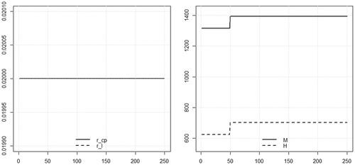This is confirmed by an examination of Figure 5, which shows that $r_{cp}$ in response to a small, 5-basis point, raise in the central bank rate, increases by only just over 3 basis points, owing to the portfolio reallocation households undertake in favor of treasury bills, the interest rate of which is tied directly to the central bank’s target rate. This result is qualitatively robust to perturbations in the values of all free parameters. Although not directly relevant to the arguments of Asensio (2017), this is an interesting implication of reproducing his assumptions in a fully-specified SFC model.

Figure 5. Effect of an increase in the interest rate on reserves.

Conclusion

The main point we wish to raise is a methodological one. Overall, our experiments suggest that while Asensio (2017) raises a number of important arguments, particularly regarding competition between bank and nonbank lending and the effects thereof on markup formation in the banking sector, some of his conclusions do not appear robust to an examination within a fully-specified (yet simple) SFC framework, even when one follows his assumptions as closely as possible. The use of a partial, non-SFC perspective leads him to ignore some important feedback effects, the inclusion of which may or may not leave his conclusions unaffected, and the consideration of which in any case allows for a better understanding of the dynamics of monetary economies. Thus, our article shows once more that, on a broader note, when dealing with monetary economics, one has to go beyond a partial equilibrium analysis that ignores feedback effects on the accumulation of assets or liabilities or on the values taken by real variables. One has to do better than moving around supply or demand curves of money or of credit, as is done for instance by Chick and Dow (2002), without considering the implications of doing so outside of a static, partial equilibrium, framework.

Notation

$sa{v}_h$	=	Household saving
$sa{v}_g$	=	Government deficit/surplus
$WB$	=	Wage bill
$F_{f/b/cb}$	=	Firm profits/Bank profits/Central Bank profits
$C/c$	=	Consumption (nominal/real)
$G/g$	=	Government expenditure (nominal/real)
$IN{V}^{\left(t\right)}/in{v}^{\left(t\right)}$	=	(Target) inventory stock (nominal/real)
$T$	=	Tax payments
$CP$	=	Commercial Paper
$L$	=	Bank loans
$H$	=	Reserves
$M$	=	Bank deposits
$G{B}_{(h/cb)}$	=	Treasury bills (held by households/central bank)
$r_{cp}$	=	Interest rate on commercial paper
$r_{gb}$	=	Interest rate on treasury bills
$r_l$	=	Interest rate on bank loans
$r_m$	=	Interest rate on bank deposits
$r_h$	=	Interest rate on reserves
$V$	=	Wealth
$Y{D}^{\left(e\right)}$	=	(Expected) disposable income
$s^{\left(e\right)}$	=	(Expected) real sales
$S/s$	=	Nominal/real sales
$Y/y$	=	Nominal/real output
${\lambda }_{ij}$	=	Portfolio choice parameters
${\alpha }_i$	=	Consumption propensities
$\psi$	=	Adaptation parameter
$p$	=	Price level
$\epsilon$	=	Commercial paper markup
${\gamma }_{inv}$	=	Target inventory to expected sales ratio
${\gamma }_1$	=	Target inventory ratio intercept
${\gamma }_1$	=	Target inventory ratio sensitivity to average interest rate
$r^{av}$	=	Average interest rate on commercial paper and bank loans
$N_d$	=	Labour demand
$\alpha$	=	Labour productivity
$w$	=	Wage rate
$UC$	=	Unit cost
$\theta$	=	Price markup over unit cost
${\chi }_{cp}$	=	Fraction of change in inventories financed by commercial paper
${\chi }_1$	=	${\chi }_b$ intercept
${\chi }_2$	=	${\chi }_b$ sensitivity to interest rate differentials
$\omega$	=	Mark-down over loan rate on bank deposits
$\tau$	=	Sales tax rate

Additional information

Notes on contributors

Marc Lavoie

Marc Lavoie, Centre d’Économie de Paris Nord (CEPN), University of Paris 13, Villetaneuse, France.

Severin Reissl

Severin Reissl, Complexity Lab in Economics (CLE), Università Cattolica del Sacro Cuore and Universität Bielefeld, Bielefeld, Germany.

Notes

1 The expression “money market interest rate” is a bit confusing as other authors close to Asensio’s position give it a different meaning. For instance, Palley (2013) uses the terms money market rate and central bank policy rate interchangeably, meaning that these terms for him correspond to the federal funds rate and its target. Asensio’s market rate or money market rate corresponds to the bond rate in the terminology of Palley (2013).

2 This is similar to one of Palley’s (2013, 417; 2017, 101) assumptions, according to whom, all else equal, an increase in the bond rate will induce an increase in loan demand.

3 It seems to us, in line with Sawyer (2017), that it is more fruitful to speak of demand and supply on a security market than to discuss the supply of and the demand for money deposits or the equilibrium of the money market.

4 All simulations were carried out using the PKSFC package for R provided by Antoine Godin, see github.com/S120/PKSFC. The model files are available at .https://github.com/SReissl/JPKE2019.

5 This simulation result was presented at a conference in Berlin in 2001, but the paper was only published in 2017!

6 This point was also made by Lavoie (2017, 371), when arguing “that the increase in inventories leads to a decrease in the share of wealth arising out of government debt, and since the steady-state income depends on the level of government expenditures, inclusive of interest payments on debt, the fall in government debt generates a fall in steady-state income.”

7 In the model, unless the central bank accepts to have a treasury bill rate which falls relative to the policy rate, this can only be achieved by a fall in the λ₂₀ coefficient, meaning that households accept to sell treasury bills with no change in their price (which is assumed to be constant and equal to 1).

8 In a corridor system, there is also no straightforward relationship between the interbank rate and the stock of reserves due to the decoupling principle, as explained by Borio and Disyatat (2010).

9 Note that we could further rewrite Equation 21 by using Equation 16 to express V_h as a function of government expenditure and the stock of treasury bills. However, we believe this presentation to be more useful in terms of intuition.

10 The initial stationary–state ratio of government debt to GDP was chosen arbitrarily and simulation results do not appear to be sensitive to changes in this initial condition.

Appendix

Further discussion of simulation results

The expressions for stationary-state income and wealth derived in the main text can be used to shed more light on the effects at work in producing the result shown in Figure 1, and in particular on what determines whether in the new stationary state, following an increase in exogenous government expenditure, the endogenous interest rates settle below or above their previous level. Recall that the markup over the central bank rate on commercial paper, which determines the level of the other endogenous interest rates in the model, is given by a rearranged portfolio equation: (15) $$\begin{array}{c}\epsilon =\frac{CP+\left({\lambda }_{13}{r}_m+{\lambda }_{12}{r}_{gb}-{\lambda }_{10}-{\lambda }_{11}{r}_h\right)V_{h,-1}+{\lambda }_{14}Y{D}^e}{{\lambda }_{11}{V}_{h,-1}}.\end{array}$$(15)

Rewriting this expression only in terms of the level of government spending $G$ and parameters to examine its derivative would result in a very lengthy and complicated expression. Instead, we rewrite the expression as follows:

First, note that the righthand side of Equation 15(15) $$\begin{array}{c}\epsilon =\frac{CP+\left({\lambda }_{13}{r}_m+{\lambda }_{12}{r}_{gb}-{\lambda }_{10}-{\lambda }_{11}{r}_h\right)V_{h,-1}+{\lambda }_{14}Y{D}^e}{{\lambda }_{11}{V}_{h,-1}}.\end{array}$$(15) contains $r_m$, which is a function of $\epsilon$; in the stationary state: $r_m=r_l-\omega =r_h+\epsilon -\omega$. Next, recall that the stationary-state output, disposable income, and consequently household wealth can be written as functions of the level of government expenditure: (16) $$\begin{array}{c}\begin{array}{c}Y=\frac{\left(G+r_{gb}GB\left[G\right]\right)\left(1+\tau \right)}{\tau },\mathrm{ }\frac{dY}{dG}\hspace{0.17em}>\hspace{0.17em}0\\ YD=\frac{\left(G+r_{gb}GB\left[G\right]\right)\left(1+\tau \right)}{\tau }\hspace{0.17em}-\hspace{0.17em}G,\mathrm{ }\frac{dYD}{dG}\hspace{0.17em}>\hspace{0.17em}0\\ V_h=\frac{\left(1-{\alpha }_1\right)YD}{{\alpha }_2}\mathrm{ }\frac{d{V}_h}{dG}\hspace{0.17em}>\hspace{0.17em}0,\end{array}\end{array}$$(16) where $GB\left[G\right]$ is used to signify that the quantity of treasury bills is itself a function of $G$ as well, which is shown in simulations to be increasing. Finally, simulations also show that the stationary-state stock of commercial paper is an increasing function of government expenditure (the exact value of which will, just like that for the stock of treasury bills, depend on the adjustment path), i.e., $\frac{dCP}{dG}>0$. Keeping this in mind and using the expression for $r_m$ presented above we rewrite Equation 15(15) $$\begin{array}{c}\epsilon =\frac{CP+\left({\lambda }_{13}{r}_m+{\lambda }_{12}{r}_{gb}-{\lambda }_{10}-{\lambda }_{11}{r}_h\right)V_{h,-1}+{\lambda }_{14}Y{D}^e}{{\lambda }_{11}{V}_{h,-1}}.\end{array}$$(15) as follows: (17) $$\begin{array}{c}\epsilon =\frac{CP-\left({\lambda }_{10}+{\lambda }_{13}\left(\omega \hspace{0.17em}-\hspace{0.17em}{r}_h\right)\hspace{0.17em}-\hspace{0.17em}{\lambda }_{12}{r}_{gb}+{\lambda }_{11}{r}_h\right)V_h+{\lambda }_{14}YD}{V_h\left({\lambda }_{11}-{\lambda }_{13}\right)},\end{array}$$(17) where we have assumed that $V_h=V_{h,-1}$ and $YD=Y{D}^e$ since we are comparing stationary states. This, in turn, enables us to rewrite the expression for $\epsilon$ as (18) $$\begin{array}{c}\epsilon =\frac{CP}{V_h\left({\lambda }_{11}-{\lambda }_{13}\right)}-\frac{\left({\lambda }_{10}+{\lambda }_{13}\left(\omega \hspace{0.17em}-\hspace{0.17em}{r}_h\right)\hspace{0.17em}-\hspace{0.17em}{\lambda }_{12}{r}_{gb}+{\lambda }_{11}{r}_h\right)}{\left({\lambda }_{11}-{\lambda }_{13}\right)}+\frac{{\lambda }_{14}YD}{V_h\left({\lambda }_{11}-{\lambda }_{13}\right)}.\end{array}$$(18)

From our discussion of the Haig-Simons consumption function above, however, we know that in the stationary state, the ratio of disposable income to household wealth is determined simply by the consumption propensities, namely (19) $$\begin{array}{c}\frac{YD}{V_h}=\frac{{\alpha }_2}{\left(1-{\alpha }_1\right)}, \end{array}$$(19) so that we finally arrive at the expression (20) $$\begin{array}{c}\epsilon =\frac{CP}{V_h\left({\lambda }_{11}-{\lambda }_{13}\right)}-\frac{\left({\lambda }_{10}+{\lambda }_{13}\left(\omega -r_h\right)-{\lambda }_{12}{r}_{gb}+{\lambda }_{11}{r}_h\right)}{\left({\lambda }_{11}-{\lambda }_{13}\right)}+\frac{{\lambda }_{14}{\alpha }_2}{\left(1-{\alpha }_1\right)\left({\lambda }_{11}-{\lambda }_{13}\right)},\end{array}$$(20) or, for simplicity, (21) $$\begin{array}{c}\epsilon =\frac{CP}{V_h\left({\lambda }_{11}-{\lambda }_{13}\right)}+z,\end{array}$$(21) where $z$ denotes the latter two fractions appearing in Equation 20(20) $$\begin{array}{c}\epsilon =\frac{CP}{V_h\left({\lambda }_{11}-{\lambda }_{13}\right)}-\frac{\left({\lambda }_{10}+{\lambda }_{13}\left(\omega -r_h\right)-{\lambda }_{12}{r}_{gb}+{\lambda }_{11}{r}_h\right)}{\left({\lambda }_{11}-{\lambda }_{13}\right)}+\frac{{\lambda }_{14}{\alpha }_2}{\left(1-{\alpha }_1\right)\left({\lambda }_{11}-{\lambda }_{13}\right)},\end{array}$$(20) which only involve parameters. This equation reinforces the intuition for the results of our experiments provided above, showing that the stationary-state level of $\epsilon$ depends on the ratio of the stock of commercial paper to the level of household wealth, that is, on the demand for nonbank credit relative to the main variable determining its supply through households’ portfolio choice.⁹⁹ Knowing that both $CP$, and $V_h$ are (positive) functions of $G$, we can then write an expression for the derivative of $\epsilon$ with respect to $G$ as follows: (22) $$\begin{array}{c}\frac{d\epsilon }{dG}=\frac{V_h\frac{dCP}{dG}-\frac{d{V}_h}{dG}CP}{({\lambda }_{11}-{\lambda }_{13})(V_h{)}^2}.\end{array}$$(22)

That is, $$\frac{d\epsilon }{dG}>0\mathrm{ }\text{iff} \frac{\raisebox{1ex}{$dCP$}\!\left/ \!\raisebox{-1ex}{$CP$}\right.}{dG}>\mathrm{ }\frac{\raisebox{1ex}{$d{V}_h$}\!\left/ \!\raisebox{-1ex}{$V_h$}\right.}{dG}$$ While the denominator of expression 22 is clearly positive since logic requires that ${\lambda }_{11}=\mathrm{ }{\lambda }_{13}\mathrm{ }{+\mathrm{ }\lambda }_{12}$ (see Godley and Lavoie 2007, 145), it does not appear possible to make a definitive judgement regarding the relative size of the two parts of the numerator (before and after the minus sign respectively). Whether the impact on the markup is positive or negative depends on whether the increase in G will generate a growth rate of corporate paper which is larger or smaller than the growth rate in household wealth. Indeed, while in the example simulation we showed above, $\frac{d\epsilon }{dG}$ was negative, we also noted that it is easy to construct a case in which the opposite result obtains (although in all cases, the effect on interest rates appears to be slight for reasonable parameter values). This demonstrates that within a fully specified SFC-framework, even when incorporating Asensio’s assumptions as far as possible, the relationship between government expenditure and interest rates, and hence the presence or absence of a crowding-out effect, is ambiguous. In particular, it will depend on the exact values taken by the derivatives of $V_h$ and $CP$ with respect to $G$ as well as the absolute values of these variables, which in turn depend on the specific values of a range of parameters.

A similar analysis can be undertaken to gain a better understanding of the effects of an increase in ${\gamma }_1$, our second experiment. Noting that, as explained in our discussion of the second experiment in the main text, the stationary-state $Y$, $YD$ and $V_h$ are decreasing functions of ${\gamma }_1$, while $CP$ is, (as one might suspect) an increasing function of ${\gamma }_1$, we obtain a derivative of $\epsilon$ with respect to ${\gamma }_1$ which looks identical to that obtained for $G$: (23) $$\begin{array}{c}\frac{d\epsilon }{d{\gamma }_1}=\frac{V_h\frac{dCP}{d{\gamma }_1}-\frac{d{V}_h}{d{\gamma }_1}CP}{({\lambda }_{11}-{\lambda }_{13})(V_h{)}^2}.\end{array}$$(23)

Once again, the denominator is clearly positive, but this time, we can also be certain about the sign of the numerator since we know that $\frac{dCP}{d{\gamma }_1}>0$ and $\frac{d{V}_h}{d{\gamma }_1}<0$. Indeed, our simulation experiments confirm that $\frac{d\epsilon }{d{\gamma }_1}$ is robustly positive. Although the result of Asensio (2017) hence appears to be confirmed in this instance, we nevertheless submit that our analysis is to be preferred since our use of a fully stock-flow consistent framework, just as argued by Godley (1999), enables us to gain a much closer understanding of the mechanisms involved in producing this outcome.

Full list of model equations

Households (24) $$\begin{array}{c}sa{v}_h=WB+F_f+F_b+r_{cp,-1} C{P}_{-1}+r_{gb,-1} G{B}_{h,-1}+r_{m,-1} M_{-1}-C\end{array}$$(24) (25) $$\begin{array}{c}{V}_h=M+CP+G{B}_h\end{array}$$(25) (26) $$\begin{array}{c}\Delta M=sa{v}_h\hspace{0.17em}-\hspace{0.17em}\Delta CP\hspace{0.17em}-\hspace{0.17em}\Delta G{B}_h\end{array}$$(26) (27) $$\begin{array}{c}YD=WB+F_f+F_b+r_{cp,-1} C{P}_{-1}+r_{gb,-1} G{B}_{h,-1}+r_{m,-1} M_{-1}\end{array}$$(27) (28) $$\begin{array}{c}Y{D}^e=Y{D}_{-1}^e+\psi \left(Y{D}_{-1}-Y{D}_{-1}^e\right)\end{array}$$(28) (29) $$\begin{array}{c}C={\alpha }_1 Y{D}^e+{\alpha }_2 V_{h,-1}\end{array}$$(29) (30) $$\begin{array}{c}c=\frac{C}{p}\end{array}$$(30) (31) $$\begin{array}{c}\epsilon =\frac{CP+\left({\lambda }_{13}\mathrm{ }{r}_m+{\lambda }_{12}\mathrm{ }{r}_{gb}\hspace{0.17em}-\hspace{0.17em}{\lambda }_{10}\hspace{0.17em}-\hspace{0.17em}{\lambda }_{11}\mathrm{ }{r}_h\right)\mathrm{ }{V}_{h,-1}+{\lambda }_{14}\mathrm{ }Y{D}^e}{{\lambda }_{11}\mathrm{ }{V}_{h,-1}}\end{array}$$(31) (32) $$\begin{array}{c}{r}_{cp}=r_h+\epsilon \end{array}$$(32) (33) $$\begin{array}{c}G{B}_h=\left({\lambda }_{20}\hspace{0.17em}-\hspace{0.17em}{\lambda }_{21}\mathrm{ }{r}_{cp}+{\lambda }_{22}\mathrm{ }{r}_{gb}-{\lambda }_{23}\mathrm{ }{r}_m\right) V_{h,-1}-\hspace{0.17em}{\lambda }_{24} Y{D}^e\end{array}$$(33)

Firms (34) $$\begin{array}{c}{F}_f=C+G+\Delta INV\hspace{0.17em}-\hspace{0.17em}T\hspace{0.17em}-\hspace{0.17em}WB\hspace{0.17em}-\hspace{0.17em}{r}_{l,-1} L_{-1}-r_{cp,-1} C{P}_{-1}\end{array}$$(34) (35) $$\begin{array}{c}{V}_f=INV\hspace{0.17em}-\hspace{0.17em}L\hspace{0.17em}-\hspace{0.17em}CP\end{array}$$(35) (36) $$\begin{array}{c}\Delta L=\Delta INV\hspace{0.17em}-\hspace{0.17em}\Delta CP\end{array}$$(36) (37) $$\begin{array}{c}s=c+g\end{array}$$(37) (38) $$\begin{array}{c}{s}^e=s_{-1}^e+\psi \left(s_{-1}\hspace{0.17em}-\hspace{0.17em}{s}_{-1}^e\right)\end{array}$$(38) (39) $$\begin{array}{c}in{v}^t={\gamma }_{inv} s^e\end{array}$$(39) (40) $$\begin{array}{c}{\gamma }_{inv}={\gamma }_1\hspace{0.17em}-\hspace{0.17em}{\gamma }_2 r^{av}\end{array}$$(40) (41) $$\begin{array}{c}y=s^e+\psi \left(in{v}^t\hspace{0.17em}-\hspace{0.17em}in{v}_{-1}\right)\end{array}$$(41) (42) $$\begin{array}{c}{r}^{av}=r_{l,-1} \frac{L_{-1}}{L_{-1}+C{P}_{-1}}+r_{cp,-1} \frac{C{P}_{-1}}{L_{-1}+C{P}_{-1}}\end{array}$$(42) (43) $$\begin{array}{c}\Delta inv=y\hspace{0.17em}-\hspace{0.17em}s\end{array}$$(43) (44) $$\begin{array}{c}{N}_d=\frac{y}{\alpha }\end{array}$$(44) (45) $$\begin{array}{c}WB=N_d w\end{array}$$(45) (46) $$\begin{array}{c}UC=\frac{w}{\alpha }\end{array}$$(46) (47) $$\begin{array}{c}p=\left(1+\theta \right) UC\end{array}$$(47) (48) $$\begin{array}{c}INV=inv UC\end{array}$$(48) (49) $$\begin{array}{c}IN{V}^t=in{v}^t UC\end{array}$$(49) (50) $$\begin{array}{c}S=s p\end{array}$$(50) (51) $$\begin{array}{c}Y=s p+\Delta inv UC\end{array}$$(51) (52) $$\begin{array}{c}\Delta CP={\chi }_{cp} \Delta INV\end{array}$$(52) (53) $$\begin{array}{c}{\chi }_{cp}=\left\{\begin{array}{cc}{\chi }_1+{\chi }_2\mathrm{ }\left(r_{l,-1}\hspace{0.17em}-\hspace{0.17em}{r}_{cp,-1}\right),& \mathrm{i}\mathrm{f}\mathrm{ }\Delta INV\ge 0\\ {\chi }_1\hspace{0.17em}-\hspace{0.17em}{\chi }_2\mathrm{ }\left(r_{l,-1}\hspace{0.17em}-\hspace{0.17em}{r}_{cp,-1}\right),& \mathrm{i}\mathrm{f}\mathrm{ }\Delta INV<0\end{array}\right.\end{array}$$(53)

Banks (54) $$\begin{array}{c}{F}_b=r_h H_{-1}+r_{l,-1} L_{-1}\hspace{0.17em}-\hspace{0.17em}{r}_{m,-1} M_{-1}\end{array}$$(54) (55) $$\begin{array}{c}{V}_b=H+L\hspace{0.17em}-\hspace{0.17em}M\end{array}$$(55) (56) $$\begin{array}{c}\Delta r_l=\psi \left(r_{cp,-1}-r_{l,-1}\right)\end{array}$$(56) (57) $$\begin{array}{c}{r}_m=r_l\hspace{0.17em}-\hspace{0.17em}\omega \end{array}$$(57)

Government (58) $$\begin{array}{c}sa{v}_g=T\hspace{0.17em}-\hspace{0.17em}G\hspace{0.17em}-\hspace{0.17em}{r}_{gb}G{B}_{-1}+F_{cb}\end{array}$$(58) (59) $$\begin{array}{c}{V}_g=-GB\end{array}$$(59) (60) $$\begin{array}{c}\Delta GB=-sa{v}_g\end{array}$$(60) (61) $$\begin{array}{c}T=\frac{\tau }{\left(1+\tau \right)} S\end{array}$$(61) (62) $$\begin{array}{c}G=gp\end{array}$$(62) (63) $$\begin{array}{c}{r}_{gb}=r_h\end{array}$$(63)

Central Bank (64) $$\begin{array}{c}{F}_{cb}=r_{gb} G{B}_{cb,-1}-r_h H_{-1}\end{array}$$(64) (65) $$\begin{array}{c}{V}_{c}b=G{B}_{cb}\hspace{0.17em}-\hspace{0.17em}H\end{array}$$(65) (66) $$\begin{array}{c}G{B}_{cb}=GB\hspace{0.17em}-\hspace{0.17em}G{B}_h\end{array}$$(66) (67) $$\begin{array}{c}H=G{B}_{cb}\end{array}$$(67)

Parameters, exogenous variables, and initial values

Initial values for the model were chosen by utilizing its stock-flow consistent structure which, together with the assumption that the simulation begins in a stationary state, helps in reducing the degrees of freedom available to the modeler in initializing a model. After setting the free parameters listed in Table 3 and imposing an initial ratio of government debt to GDP as listed in Table 4,¹⁰ all necessary initial values of stocks and flows are implied by the SFC structure of the model, jointly with the imposition of an initial stationary state.

Table 3. Parameters and exogenous variables.

Parameter	Value	Parameter	Value	Parameter	Value
χ1	0.5	χ2	1000	τ	0.25
γ1	1.45	γ2	2.5	θ	0.5
α	1	ψ	0.5	α1	0.875
α2	0.05	ω	0.01	λ10	0.27727
λ11	2.5	λ12	1.25	λ13	1.25
λ14	0.2	λ20	0.45	λ21	1.25
λ22	2.5	λ23	1.25	λ24	0.2
g	200	rh	0.005	w	1

Table 4. Initial values.

Variable	Initial value	Variable	Initial value	Variable	Initial value
inv	1419.5887	INV	1419.5887	s	1028.2776
se3	1028.2776	YD	1242.4165	YD^e	1242.4165
Vh	3106.0411	rm	0.01	rl	0.02
rcp	0.02	M	1324.6626	CP	709.7943
GB	1696.6581	GBh	1071.5842	GBcb	625.0739
L	709.7943	H	625.0739

Note. All figures were created in R. All tables were created in Word.

Where possible, the values of the free parameters and exogenous variables were chosen broadly in line with the existing literature; otherwise they were set to values which appear reasonable. The value of λ1₀ is implied as a residual by the initialization. The choice of G is arbitrary, but its magnitude merely has an effect on the levels of other model variables (especially income) and does not affect dynamic or comparative static results. w and α were normalized to 1 for convenience. Where the choice of parameter values has an effect on our simulation results, this was detailed in the main text.

An alternative specification

As pointed out earlier, there is evidence that the prime lending rate is set as a given markup on the target interest rate set by the central bank. Keeping in mind that the bank lending rate and the commercial paper rate should gravitate around each other, this would imply that there is a one-way causality and that the commercial paper rate tends towards the exogenously-determined interest rate on bank loans. To obtain convergence one needs to replace Equation 4 with an equation that says that firms now reallocate a fraction of their entire financing needs (including refinancing and any changes in inventories) between commercial paper and bank loans as a function of the interest rate differential. This seems like a realistic feature to introduce since both corporate paper and bank loans mature within one or a few periods, allowing firms to switch part of their stock of borrowed funds from one form to another. In this case, we have verified that, following a shock, the commercial paper rate can diverge from the (now exogenous) interest rate on bank loans, but that it eventually returns to being equal to the interest rate on bank loans.

References

- Asensio, A. 2017. “Insights on Endogenous Money and the Liquidity Preference Theory of Interest.” Journal of Post Keynesian Economics 40 (3):327–48. doi:10.1080/01603477.2017.1319248.
- Borio, C., and P. Disyatat. 2010. “Unconventional Monetary Policies: An Appraisal.” The Manchester School 78 (s1):53–89. doi:10.1111/j.1467-9957.2010.02199.x.
- Caverzasi, E., and A. Godin. 2015. “Post-Keynesian Stock-Flow-Consistent Modelling: A Survey.” Cambridge Journal of Economics 39 (1):157–87. doi:10.1093/cje/beu021.
- Chick, V., and S. C. Dow. 2002. “Monetary Policy with Endogenous Money and Liquidity Preference: A Nondualistic Treatment.” Journal of Post Keynesian Economics 24 (4):587–607. doi:10.1080/01603477.2002.11490345.
- Fontana, G., and M. Setterfield. 2009. “A Simple (and Teachable) Macroeconomic Model with Endogenous Money.” In Macroeconomic Theory and Macroeconomic Pedagogy, edited by G. Fontana and M. Setterfield, 144–68. Basingstoke: Palgrave Macmillan.
- Godley, W. 1999. “Money and Credit in a Keynesian Model of Income Determination.” Cambridge Journal of Economics 23 (4):393–411. doi:10.1093/cje/23.4.393.
- Godley, W., and M. Lavoie. 2007. Monetary Economics - an Integrated Approach to Credit, Money, Income, Production and Wealth. Basingstoke: Palgrave Macmillan.
- Howells, P. 2009. “Money and Banking.” In A Realistic Macro Model.” in Macroeconomic Theory and Macroeconomic Pedagogy, edited by G. Fontana and M. Setterfield, 169–81. Basingstoke: Palgrave Macmillan.
- Keynes, J. M. 1936. The General Theory of Employment, Interest and Money. London: Macmillan.
- Lavoie, M. 2010. “Changes in Central Bank Procedures during the Subprime Crisis and Their Repercussions on Monetary Theory.” International Journal of Political Economy 39 (3):3–23. doi:10.2753/IJP0891-1916390301.
- Lavoie, M. 2014. Post-Keynesian Economics - New Foundations. Cheltenham: Edward Elgar.
- Lavoie, M. 2016. “Understanding the Global Financial Crisis: Contributions of Post-Keynesian Economics.” Studies in Political Economy 97 (1):58–75.
- Lavoie, M. 2017. “Assessing Some Structuralist Claims Through a Coherent Stock-Flow Consistent Framework.” In Advances in Endogenous Money Analysis, edited by L.-P. Rochon and S. Rossi, 353–78. Cheltenham: Edward Elgar.
- Lavoie, M., and W. Godley. 2001. 02. “Kaleckian Models of Growth in a Coherent Stock-Flow Monetary Framework: A Kaldorian View.” Journal of Post Keynesian Economics 24 (2):277–311. doi:10.1080/01603477.2001.11490327.
- Nikiforos, M., and G. Zezza. 2017. “Stock-Flow Consistent Macroeconomic Models: A Survey.” Journal of Economic Surveys 31 (5):1204–39. doi:10.1111/joes.12221.
- Palley, T. I. 2013. “Horizontalists, Verticalists, and Structuralists: The Theory of Endogenous Money Reassessed.” Review of Keynesian Economics 1 (4):406–24. doi:10.4337/roke.2013.04.03.
- Palley, T. I. 2017. “The Theory of Endogenous Money and the LM Schedule: Prelude to a Reconstruction of IS-LM.” In Advances in Endogenous Money Analysis, edited by L.-P. Rochon and S. Rossi, 88–110. Cheltenham: Edward Elgar.
- Sawyer, M. 2017. “Endogenous Money and the Tyranny of Demand and Supply.” In Advances in Endogenous Money Analysis, edited by L.-P. Rochon and S. Rossi, 227–44. Cheltenham: Edward Elgar.