Functional income distribution, effective demand and wealth in Denmark – insights from an empirical stock-flow consistent model

Abstract

With the important contribution of Marglin and Bhaduri different demand and growth regimes were identified, which inspired a strand of empirical research aiming to uncover the type of growth regime. Most of these studies can be framed into two methodological approaches: (i) a structural, and (ii) an aggregative approach. In this paper, we use a third approach where we exploit the advantages of the stock-flow consistent framework. We argue that using an empirical SFC model retains the advantages of the two more widely used approaches, while adding some novel features: (i) the endogenization of income distribution, which allows for a two-way relationship between demand and income shares, (ii) the consistent incorporation of stock variables in the estimation of the equations of aggregate demand components, and (iii) the inclusion of endogenous labor market dynamics in the analysis. To introduce these features, we build an empirical stock-flow consistent model for Denmark for the period 2005q1–2020q1. Our analysis suggests that demand can neither be categorically defined as wage-led nor profit-led, as the effects of a change in income distribution on the aggregate demand components cancel each other out. Results are more conclusive for capital accumulation, which is found to be profit-led.

Keywords:

• Demand and growth regimes
• stock-flow consistent models
• Denmark

JEL CLASSIFICATION CODES:

• E12
• E25
• E57
• E01

Introduction

The relationship between income distribution, aggregate demand and capital accumulation has received a lot of attention within Post-Keynesian theory (see Bowles and Boyer 1988; Dutt 1984; Rowthorn 1981). In the basic Kaleckian distribution and growth model, an increase in the profit share is assumed to have a negative effect on both the demand and accumulation of capital, implying that the economy is wage-led. With the important contributions of Blecker (1989), Bhaduri and Marglin (1990), and Marglin & Bhaduri (1991), different regimes of growth and demand were introduced, which led to an increasing number of empirical studies analyzing whether a given economy can be characterized as profit-led or wage-led (see Hein and Vogel 2007; Onaran and Obst 2016; Storm and Naastepad 2012; Stockhammer and Wildauer 2016). In a nutshell, an economy is considered to be wage-led, if an increase in wage share leads to an increase in the overall economic activity. In contrast, an economy is considered to be profit-led, if an increase in wage share leads to a decline in the overall economic activity.

At the empirical level, two main strategies have been followed to identify the underlying demand regime of an economy. On the one hand, the so-called “structural” approach assesses the individual components of aggregate demand using separate econometric estimations, where the wage share is taken as an exogenous explanatory variable. The effect of a change in income distribution on aggregate demand is obtained by summing up the effects of this change on consumption, investment, and net exports.¹ On the other hand, the “aggregative” approach consists of a single econometric estimation of aggregate demand on the wage share and a set of control variables related to the individual components of aggregate demand. In this approach, the sign of the coefficient attached to the wage share determines whether the economy is wage-led or profit-led.²

The main strength of the structural approach is that it allows for the measurement of the relevance of each individual component of aggregate demand on short-term dynamics, as well as the effects of changes in income distribution. However, the estimation of separate equations omits the possible dynamic interactions between the variables³ (for instance, the accelerator effect). Moreover, the fact that income distribution enters the estimations as an exogenous variable, misses out on the feedback effects from demand to income distribution, as discussed in Skott (2017). The aggregative approach, for its part, has the strength of addressing the simultaneity between demand and distribution and the dynamic interactions between the variables that the structural approach, by construction, excludes. However, the aggregative nature of the framework prevents it from distinguishing which components of demand are more relevant, thereby reducing its capacity to draw conclusions regarding the most important drivers of the underlying dynamics.⁴

In this paper, we contribute to the literature on demand regimes by examining the growth regimes for the Danish economy using an empirical model following the stock-flow-consistent framework. Specifically, we build an empirical stock-flow-consistent model for Denmark using quarterly data from 2005q1 to 2020q1. We exploit the dynamics of the model to explore whether the economy can be explicitly classified as profit-led or wage-led. Despite being one of the core modeling approaches in the field of heterodox economics, to the best of our knowledge, there are no studies that explicitly address the question of demand regimes in a fully-fledged empirical SFC model. This approach not only combines the strengths of the two other approaches but also provides further insights. Firstly, while making use of the diversity of transactions embedded in the economy, SFC models retain the advantages of the “structural” approach and even enhances it through the wide range of processes that are modeled beyond the aggregate demand equations. Secondly, even if the structural parameters are estimated using a single equation method, the fact that the model is solved as a system of simultaneous equations implies that the variables can affect each other in such a way that the dynamic effects captured in the “aggregative” approach are present.⁵ Finally, SFC models capture the stock-flow interactions in a consistent way, which allows us to uncover important insights that are beyond the scope of models which are non-stock-flow-consistent in nature.

The rest of the paper is organized as follows. “Theory” section presents the theoretical framework regarding demand regimes used in the Post-Keynesian literature, and reviews some empirical studies of the Danish economy. “Model and data” section presents the main features of our empirical model. In “Analysis and discussion” section, we make an experiment in relation to functional income distribution and analyze its impact on some of the key variables. “Conclusions” section concludes this paper.

Theory

The analytical framework provided in Bhaduri and Marglin (1990) and Marglin & Bhaduri (1990) arguably serves as a foundation for many post-Keynesian investigations of whether a given economy is wage-led or profit-led. We begin by presenting a theoretical framework for analyzing an open economy following the description in Hein (2014), to which we add some special features that characterize the empirical SFC model used in the remainder of this paper.

A post-Keynesian model of growth and distribution

We assume a small open economy with a public sector where both workers and capitalists are saving out of their disposable income, and define $\mathit{\Pi }$ as nominal gross profits, $Y$ as real income, $p$ as the price index, $s_W$ as the saving rate out of wages net of taxes, $s_{\mathit{\Pi }}$ as the saving rate out of profit plus property income net of taxes. ${\theta }_W$ and ${\theta }_{\mathit{\Pi }}$ are the income tax rates, $A$ as the stock of assets held by upper-income households and $r$ as the interest rate earned on these assets (the share c of the stock of assets is held in foreign debt and the share 1-c in public debt). Aggregate saving is then given by: (1) $$S=S_{\mathit{\Pi }}+S_W=s_{\mathit{\Pi }}\left[\mathit{\Pi }+\mathit{\text{rA}}\right]\left(1-{\theta }_{\mathit{\Pi }}\right)+s_W\left[\left(\mathit{\text{Yp}}-\mathit{\Pi }\right)\left(1-{\theta }_W\right)\right]$$(1) where $0\le s_W<s_{\mathit{\Pi }}\le 1.$

Defining $\pi =\frac{\mathit{\Pi }}{\mathit{\text{pY}}}$ as the profit share, $u=\frac{Y}{Y^n}$ as the rate of capacity utilization (where $Y^n$ is the “normal” or long-run level of output), and $v=\frac{K}{Y^n}$ the technologically determined capital to potential-output ratio, we can express savings in terms of the nominal stock of capital. When doing so, we will define $a=\frac{A}{\mathit{\text{pK}}}$ as the ratio of assets to the stock of capital. The total rate of saving, s, can be written as: (2) $$s=\frac{S}{\mathit{\text{pK}}}=\left[s_{\mathit{\Pi }}\pi \left(1-{\theta }_{\mathit{\Pi }}\right)+s_W\left(1-\pi \left(1-{\theta }_W\right)-{\theta }_W\right)\right]\mathrm{*}\frac{u}{v}+s_{\mathit{\Pi }}\mathit{\text{ra}}\left(1-{\theta }_{\mathit{\Pi }}\right)$$(2)

Investment is defined as done by Hein (2014), where the rate of accumulation is assumed to be a function of the animal spirits, capacity utilization, and the profit share. To link investment decisions to the financial sphere of the economy – which is one of the salient features of SFC models – we augment the investment equation by including a proxy of Tobin’s “q”, which in turn can be computed as the ratio of the market value of the outstanding stock of shares to the nominal capital stock. (3) $$g=\frac{I}{K}=i_0+i_1\pi +i_{2}u+i_{3}q\mathrm{ }$$(3)

Domestic prices are set by firms as a markup (m) over labor costs ($w\frac{L}{Y}$) and imported materials ($p_{f}e\mu$). To simplify the price equation, the term $z=\frac{p_{f}e\mu }{w\frac{L}{Y}}$ is defined, which captures the relationship between unit material costs and unit labor costs. Domestic prices can then be written as: (4) $$p=\left(1+m\right)w\frac{L}{Y}\left(1+z\right)$$(4)

The markup is mainly being determined by a combination of the degree of competition in the goods market and the unions’ bargaining power in the labor market. Thus, income distribution is given by the markup and z: (5) $$\pi =\frac{\mathit{\Pi }}{Y}=\frac{\mathit{\Pi }}{\mathit{\Pi }+W}=\frac{\left(1+z\right)m}{1+\left(1+z\right)m}=\frac{1}{\frac{1}{\left(1+z\right)m}+1}$$(5)

Net exports are defined as a function of the real exchange rate ($\mathit{\text{rer}}$), the level of activity of the rest of the world ($u_f$) and the domestic rate of capacity utilization ($u$). If interest earned on capital (or property) income ($\mathit{\text{rca}}$) is added to net exports, the current account balance (B) is obtained. It is convenient to scale the current account by the nominal stock of capital ($b=\frac{B}{\mathit{\text{pK}}}$), leading to the following expression. (6) $$b={\mathit{\text{nx}}}_1\mathrm{*}\mathit{\text{rer}}\left(\pi \right)+{\mathit{\text{nx}}}_2\mathrm{*}{u}_f-{\mathit{\text{nx}}}_3\mathrm{*}u+\mathit{\text{rca}}$$(6)

The real exchange rate is a function of profit share, capturing the negative relationship between the latter and unit costs (which are a proxy of competitiveness). The real exchange rate is expressed as the domestic currency in terms of foreign currency. Unit costs and the markup enter the real exchange rate equation through the domestic price level. (7) $$\mathit{\text{rer}}=\frac{\mathit{\text{ep}}}{p_f}$$(7)

The government’s deficit is given by expenditures $\mathit{\text{pZ}}$ plus interest payments, $r\left(1-c\right)A,$ minus tax income, $T.$ Based on the separate income tax rates defined above, the deficit can be expressed as follows: (8) $$D=\mathit{\text{Zp}}+r\left(1-c\right)A-{\theta }_W\left(\mathit{\text{Yp}}-\mathit{\Pi }\right)-{\theta }_{\mathit{\Pi }}\left(\mathit{\Pi }+\mathit{\text{rA}}\right)$$(8)

Scaling the deficit by the nominal stock of capital and defining $z=\frac{Z}{K}$ as the public consumption-to-capital ratio we get: (9) $$d=\frac{u}{v}\left[{\theta }_W\left(\pi -1\right)-{\theta }_{\mathit{\Pi }}\pi \right]+\mathit{\text{ra}}\left[\left(1-c\right)-{\theta }_{\mathit{\Pi }}\right]+z$$(9)

The equilibrium in the goods market requires that: (10) $$s=g+b+d$$(10)

Inserting Equations (2) (3) (6) and (9) into (10), we obtain the equilibrium rate of capacity utilization.⁶ (11) $$u^{\mathrm{*}}=\frac{v\left\{i_0+i_1\pi +i_{3}q{+\mathit{\text{nx}}}_1\mathrm{\hspace{0.17em}}\mathrm{*}\mathrm{\hspace{0.17em}}\mathit{\text{rer}}+{\mathit{\text{nx}}}_2\mathrm{\hspace{0.17em}}\mathrm{*}\mathrm{\hspace{0.17em}}{u}_f+z+\mathit{\text{ra}}\left(1-{\theta }_{\mathit{\Pi }}\right)\left(1-s_{\mathit{\Pi }}\right)\right\}}{\pi \left[s_{\mathit{\Pi }}\left(1-{\theta }_{\mathit{\Pi }}\right)+s_W\left({\theta }_W-1\right)+{\theta }_W-{\theta }_{\mathit{\Pi }}\right]+s_W\left({1-\theta }_W\right)-{\theta }_W+v\left({\mathit{\text{nx}}}_3-i_2\right)}$$(11)

Plugging the expression for $u^{\mathrm{*}}$ in Equation (3)(1) $$S=S_{\mathit{\Pi }}+S_W=s_{\mathit{\Pi }}\left[\mathit{\Pi }+\mathit{\text{rA}}\right]\left(1-{\theta }_{\mathit{\Pi }}\right)+s_W\left[\left(\mathit{\text{Yp}}-\mathit{\Pi }\right)\left(1-{\theta }_W\right)\right]$$(1) , we get the equilibrium rate of accumulation. (12) $$g^{\mathrm{*}}=\frac{\begin{array}{c}\left[i_0+i_1\pi +i_{3}q\right]⟨\pi \left[s_{\mathit{\Pi }}\left(1-{\theta }_{\mathit{\Pi }}\right)+s_W\left({\theta }_W-1\right)+{\theta }_W-{\theta }_{\mathit{\Pi }}\right]+s_W\left({1-\theta }_W\right)\\ -{\theta }_W+v\left({\mathit{\text{nx}}}_3-i_2\right)⟩+i_{2}v\left[{\mathit{\text{nx}}}_1\mathrm{\hspace{0.17em}}\mathrm{*}\mathrm{\hspace{0.17em}}\mathit{\text{rer}}+{\mathit{\text{nx}}}_2\mathrm{\hspace{0.17em}}\mathrm{*}\mathrm{\hspace{0.17em}}{u}_f+z+\mathit{\text{ra}}\left(1-{\theta }_{\mathit{\Pi }}\right)\left(1-s_{\mathit{\Pi }}\right)\right]\end{array}}{\pi \left[s_{\mathit{\Pi }}\left(1-{\theta }_{\mathit{\Pi }}\right)+s_W\left({\theta }_W-1\right)+{\theta }_W-{\theta }_{\mathit{\Pi }}\right]+s_W\left({1-\theta }_W\right)-{\theta }_W+v\left({\mathit{\text{nx}}}_3-i_2\right)}$$(12)

With the short run equilibrium values for capacity utilization and the rate of accumulation we can explore the effect of a change in income distribution and capital accumulation by taking the derivatives (see Appendix B) with respect to the profit share, which provides four different possible regimes:

If $\frac{\partial u^{\mathrm{*}}}{\partial \pi }>0$ and $\frac{\partial g^{\mathrm{*}}}{\partial \pi }>0,$ then the economy would exhibit a fully-fledged profit-led regime.

If $\frac{\partial u^{\mathrm{*}}}{\partial \pi }<0$ and $\frac{\partial g^{\mathrm{*}}}{\partial \pi }<0,$ then the economy would exhibit a fully-fledged wage-led regime

If $\frac{\partial u^{\mathrm{*}}}{\partial \pi }<0$ and $\frac{\partial g^{\mathrm{*}}}{\partial \pi }>0,$ then a wage-led demand regime and a profit-led growth regime can be identified.

If $\frac{\partial u^{\mathrm{*}}}{\partial \pi }>0$ and $\frac{\partial g^{\mathrm{*}}}{\partial \pi }<0,$ then a profit-led demand regime and a wage-led growth regime can be identified.

Based on Equation (B3)(B3) $$\frac{\partial u^{\mathrm{*}}}{\partial \pi }=\frac{\begin{array}{c}v{i}_1⟨\pi \left[s_{\mathit{\Pi }}\left(1-{\theta }_{\mathit{\Pi }}\right)+s_W\left({\theta }_W-1\right)+{\theta }_W-{\theta }_{\mathit{\Pi }}\right]+s_W\left({1-\theta }_W\right)-{\theta }_W+v\left({\mathit{\text{nx}}}_3-i_2\right)⟩\hfill \\ -v\{i_0+i_1\pi +i_{3}q{+\mathit{\text{nx}}}_1\mathrm{\hspace{0.17em}}\mathrm{*}\mathrm{\hspace{0.17em}}\mathit{\text{rer}}+{\mathit{\text{nx}}}_2\mathrm{\hspace{0.17em}}\mathrm{*}\mathrm{\hspace{0.17em}}{u}_f+z+\mathit{\text{ra}}\left(1-{\theta }_{\mathit{\Pi }}\right)\left(1-s_{\mathit{\Pi }}\right)\}\\ \left[s_{\mathit{\Pi }}\left(1-{\theta }_{\mathit{\Pi }}\right)+s_W\left({\theta }_W-1\right)+{\theta }_W-{\theta }_{\mathit{\Pi }}\right]\end{array}}{{⟨\pi \left[s_{\mathit{\Pi }}\left(1-{\theta }_{\mathit{\Pi }}\right)+s_W\left({\theta }_W-1\right)+{\theta }_W-{\theta }_{\mathit{\Pi }}\right]+s_W\left({1-\theta }_W\right)-{\theta }_W+v\left({\mathit{\text{nx}}}_3-i_2\right)⟩}^2}$$(B3) , a wage-led demand regime would require that: (13) $$i_1<\frac{i_0+i_{3}q{+\mathit{\text{nx}}}_1\mathrm{\hspace{0.17em}}\mathrm{*}\mathrm{\hspace{0.17em}}\mathit{\text{rer}}+{\mathit{\text{nx}}}_2\mathrm{\hspace{0.17em}}\mathrm{*}\mathrm{\hspace{0.17em}}{u}_f+z+\mathit{\text{ra}}\left(1-{\theta }_{\mathit{\Pi }}\right)\left(1-s_{\mathit{\Pi }}\right)}{s_W\left({1-\theta }_W\right)-{\theta }_W+v\left({\mathit{\text{nx}}}_3-i_2\right)}$$(13)

From Equation (B4)(B4) $$\frac{\partial g^{\mathrm{*}}}{\partial \pi }=\frac{\begin{array}{l}\{\left[s_{\mathit{\Pi }}\left(1-{\theta }_{\mathit{\Pi }}\right)+s_W\left({\theta }_W-1\right)+{\theta }_W-{\theta }_{\mathit{\Pi }}\right]\left[i_0+{2i}_1\pi +i_{3}q\right]\\ +i_1\left[s_W\left({1-\theta }_W\right)-{\theta }_W+v\left({\mathit{\text{nx}}}_3-i_2\right)\right]\}[\pi \left[s_{\mathit{\Pi }}\left(1-{\theta }_{\mathit{\Pi }}\right)+s_W\left({\theta }_W-1\right)+{\theta }_W-{\theta }_{\mathit{\Pi }}\right]\\ +s_W\left({1-\theta }_W\right)-{\theta }_W+v\left({\mathit{\text{nx}}}_3-i_2\right)]\end{array}}{{⟨\pi \left[s_{\mathit{\Pi }}\left(1-{\theta }_{\mathit{\Pi }}\right)+s_W\left({\theta }_W-1\right)+{\theta }_W-{\theta }_{\mathit{\Pi }}\right]+s_W\left({1-\theta }_W\right)-{\theta }_W+v\left({\mathit{\text{nx}}}_3-i_2\right)⟩}^2}-\frac{-\left\{\left[i_0+i_1\pi +i_{3}q\right]⟨\pi \left[s_{\mathit{\Pi }}\left(1-{\theta }_{\mathit{\Pi }}\right)+s_W\left({\theta }_W-1\right)+{\theta }_W-{\theta }_{\mathit{\Pi }}\right]+s_W\left({1-\theta }_W\right)-{\theta }_W+v\left({\mathit{\text{nx}}}_3-i_2\right)⟩\right\}}{{⟨\pi \left[s_{\mathit{\Pi }}\left(1-{\theta }_{\mathit{\Pi }}\right)+s_W\left({\theta }_W-1\right)+{\theta }_W-{\theta }_{\mathit{\Pi }}\right]+s_W\left({1-\theta }_W\right)-{\theta }_W+v\left({\mathit{\text{nx}}}_3-i_2\right)⟩}^2}+\frac{+i_{2}v\left[{\mathit{\text{nx}}}_1\mathrm{\hspace{0.17em}}\mathrm{*}\mathrm{\hspace{0.17em}}\mathit{\text{rer}}+{\mathit{\text{nx}}}_2\mathrm{\hspace{0.17em}}\mathrm{*}\mathrm{\hspace{0.17em}}{u}_f+z+\mathit{\text{ra}}\left(1-{\theta }_{\mathit{\Pi }}\right)\left(1-s_{\mathit{\Pi }}\right)\right]\left[s_{\mathit{\Pi }}\left(1-{\theta }_{\mathit{\Pi }}\right)+s_W\left({\theta }_W-1\right)+{\theta }_W-{\theta }_{\mathit{\Pi }}\right]}{{⟨\pi \left[s_{\mathit{\Pi }}\left(1-{\theta }_{\mathit{\Pi }}\right)+s_W\left({\theta }_W-1\right)+{\theta }_W-{\theta }_{\mathit{\Pi }}\right]+s_W\left({1-\theta }_W\right)-{\theta }_W+v\left({\mathit{\text{nx}}}_3-i_2\right)⟩}^2}$$(B4) , it is derived that a wage-led growth regime would require that: (14) $$i_1<\frac{\begin{array}{c}\left[i_0+i_{3}q\right]\left[s_W\left({1-\theta }_W\right)-{\theta }_W+v\left({\mathit{\text{nx}}}_3-i_2\right)\right]+i_{2}v\left[{\mathit{\text{nx}}}_1\mathrm{\hspace{0.17em}}\mathrm{*}\mathrm{\hspace{0.17em}}\mathit{\text{rer}}+{\mathit{\text{nx}}}_2\mathrm{\hspace{0.17em}}\mathrm{*}\mathrm{\hspace{0.17em}}{u}_f+z+\mathit{\text{ra}}\left(1-{\theta }_{\mathit{\Pi }}\right)\left(1-s_{\mathit{\Pi }}\right)\right]\\ \left[s_{\mathit{\Pi }}\left(1-{\theta }_{\mathit{\Pi }}\right)+s_W\left({\theta }_W-1\right)+{\theta }_W-{\theta }_{\mathit{\Pi }}\right]\end{array}}{{\pi }^2\left\{\left[s_{\mathit{\Pi }}\left(1-{\theta }_{\mathit{\Pi }}\right)+s_W\left({\theta }_W-1\right)+{\theta }_W-{\theta }_{\mathit{\Pi }}\right]+\left[s_W\left({1-\theta }_W\right)-{\theta }_W+v\left({\mathit{\text{nx}}}_3-i_2\right)\right]\right\}\left\{2\left(\left[s_{\mathit{\Pi }}\left(1-{\theta }_{\mathit{\Pi }}\right)+s_W\left({\theta }_W-1\right)+{\theta }_W-{\theta }_{\mathit{\Pi }}\right]+\left[s_W\left({1-\theta }_W\right)-{\theta }_W+v\left({\mathit{\text{nx}}}_3-i_2\right)\right]-1\right)\right\}}$$(14)

Equations (13)(13) $$i_1<\frac{i_0+i_{3}q{+\mathit{\text{nx}}}_1\mathrm{\hspace{0.17em}}\mathrm{*}\mathrm{\hspace{0.17em}}\mathit{\text{rer}}+{\mathit{\text{nx}}}_2\mathrm{\hspace{0.17em}}\mathrm{*}\mathrm{\hspace{0.17em}}{u}_f+z+\mathit{\text{ra}}\left(1-{\theta }_{\mathit{\Pi }}\right)\left(1-s_{\mathit{\Pi }}\right)}{s_W\left({1-\theta }_W\right)-{\theta }_W+v\left({\mathit{\text{nx}}}_3-i_2\right)}$$(13) and (14)(14) $$i_1<\frac{\begin{array}{c}\left[i_0+i_{3}q\right]\left[s_W\left({1-\theta }_W\right)-{\theta }_W+v\left({\mathit{\text{nx}}}_3-i_2\right)\right]+i_{2}v\left[{\mathit{\text{nx}}}_1\mathrm{\hspace{0.17em}}\mathrm{*}\mathrm{\hspace{0.17em}}\mathit{\text{rer}}+{\mathit{\text{nx}}}_2\mathrm{\hspace{0.17em}}\mathrm{*}\mathrm{\hspace{0.17em}}{u}_f+z+\mathit{\text{ra}}\left(1-{\theta }_{\mathit{\Pi }}\right)\left(1-s_{\mathit{\Pi }}\right)\right]\\ \left[s_{\mathit{\Pi }}\left(1-{\theta }_{\mathit{\Pi }}\right)+s_W\left({\theta }_W-1\right)+{\theta }_W-{\theta }_{\mathit{\Pi }}\right]\end{array}}{{\pi }^2\left\{\left[s_{\mathit{\Pi }}\left(1-{\theta }_{\mathit{\Pi }}\right)+s_W\left({\theta }_W-1\right)+{\theta }_W-{\theta }_{\mathit{\Pi }}\right]+\left[s_W\left({1-\theta }_W\right)-{\theta }_W+v\left({\mathit{\text{nx}}}_3-i_2\right)\right]\right\}\left\{2\left(\left[s_{\mathit{\Pi }}\left(1-{\theta }_{\mathit{\Pi }}\right)+s_W\left({\theta }_W-1\right)+{\theta }_W-{\theta }_{\mathit{\Pi }}\right]+\left[s_W\left({1-\theta }_W\right)-{\theta }_W+v\left({\mathit{\text{nx}}}_3-i_2\right)\right]-1\right)\right\}}$$(14) define the conditions (in terms of the value of the sensitivity of capital accumulation to the profit share) that would make the economy fully-fledged wage-led, meaning that both demand and growth are negatively affected by an increase in the profit share. Given the large number of determinants found in these equations, there is a large variety of structural, institutional, and policy-related factors that play a role in the configuration of the underlying regime. The same applies to the effect that a change in income distribution would have on the current account and the government’s balance. This implies that the question of the impact of distribution patterns on the performance of an economy needs to be ultimately solved empirically. With this motivation we attempt to contribute to this research agenda through a modeling methodology that is capable of accounting for the diversity of factors that define the demand and growth regime of an economy.

Denmark’s macroeconomic regime(s)

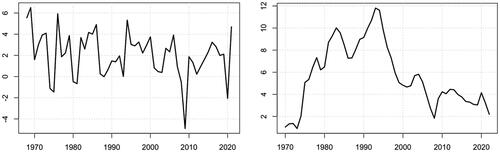
Prior to discussing whether the Danish economy can be categorized as wage-led or profit-led, we provide a brief overview of the relevant macroeconomic developments. The Danish economy has experienced modest economic growth since the 1970s. The overall economy is generally quite resilient to adverse shocks as is evident by the quick recovery in GDP growth and unemployment rate following the impact of the two well-known crises (see, Figure 1(a,b)).

Figure 1. (a) Real GDP growth. (b) Unemployment rate.

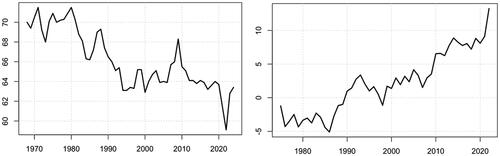
Focusing on functional income distribution, Figure 2a shows that the adjusted wage share has declined over the long run, which to some extent fits the description of financialization theory. Furthermore, Denmark has accumulated a large stock for foreign wealth due to persistent current account surpluses since the late 1980s as shown in Figure 2b, and thereby fits the description of an export-led growth as described by Dodig, Hein, and Detzer (2016).

Figure 2. (a) Adjusted wage share. (b) Current account to GDP.

Turning to the question of whether the Danish economy can be characterized as wage-led or profit-led, the literature in this regard is limited. Denmark is usually covered as a side story in a panel of several countries and the conclusion to date remains ambiguous. In Onaran and Obst (2016), who provide an analysis for the period 1960–2013 using the “structural approach”, Denmark is found to be profit-led. This result is driven by the fact that the relative effect of income distribution on investment exceeds the effect on consumption, which makes the Danish economy profit-led even before adding net exports to the analysis.⁷ Unsurprisingly, adding the effect of net export strengthens their conclusion that Denmark is profit-led. Oyvat, Öztunalı, and Elgin (2020) explore this question by estimating an ARDL model for Denmark, on the grounds that they are interested in long-run relationships between the wage share and GDP. They find the long run coefficient to be negative indicating the Danish economy to be profit-led. They use the same AMECO database as Onaran and Obst (2016), but for the period 1964 to 2011.

There are, however, other studies that find Denmark to be wage-led. For instance, Obst, Onaran, and Nikolaidi (2017) use the same database as their 2016 paper for the period 1960–2013 and apply the “structural approach” to which they add fiscal policy. Due to the incorporation of tax rates in the model, the effect of a change in income distribution on consumption increases compared to studies where no tax rates are included, which causes Denmark to switch from being profit-led to wage-led. Storm and Naastepad (2012) find the Danish economy to be wage-led for the period 1960–2000, which is mainly due to stronger effects of changes in income distribution on consumption than on net exports. In a recent study, Bengtsson and Stockhammer (2021) conclude that the Danish economy was weakly wage-led in the period going from 1900 to 2010. In the second part of their analysis, they focus on the period after WWII, where the effect of an increase in the wage share on the economic growth is stronger, which supports the wage-led nature of the Danish economy.

Given the small number of empirical studies investigating the Danish economy, the claim from Blecker (2016) that the empirical literature has not yet reached a consensus regarding whether a given economy is wage-led or profit-led might apply to Denmark.

Model and data

In order to further explore the question of the growth regime in Denmark, we use an empirical Stock-Flow-Consistent (SFC) model, which allows us (i) endogenizing the distribution of income by defining separate price and wage equations allows for a series of feedback mechanisms between aggregated demand and the distribution of income that might play a relevant role in the dynamics. (ii) By expanding the analysis to include the balance sheet effects, which are likely to play an important when discussing income distribution. (iii) By explicitly including the labor market in the analysis, we are able to account for any feedback mechanism between the labor market and the goods market.

In what follows, we explain the data and the main assumptions used while building the model, before diving into the details of its structure.⁸ The model is estimated from quarterly data for Denmark for the period 2005q1 to 2020q1. To construct the model, equations involving structural parameters are estimated using dynamic OLS regressions. After de-seasonalising the data, we test the variables for stationarity and then explore the dynamic relationship between our variables of interest. In most cases, the structural parameters are estimated using the ARDL bounds test. A general-to-specific methodology is followed, where we start with a large number of lags and then drop the irrelevant ones such that the final version of the model is more parsimonious. Even though our estimation strategy attempts to choose a model structure that best fits the data for a given dependent variable, economic theory is the main guiding light when defining which explanatory variables enter the equation.⁹

The model describes Denmark as a small open economy with a fixed exchange rate regime. The small open economy assumption implies that the variables related to the rest of the world, like foreign interest rates, rest of the world economic activity and prices, are kept exogenous.

We assume Denmark to be a mature economy, where labor market restrictions are taken into account. Thus, wages and therefore prices are assumed to be affected by changes in the rate of unemployment (there is no “reserve army” allowing for increases in employment having a neutral effect on the real wage).

Following the system of national accounts, the rest of the world, households, nonfinancial corporations, financial corporations, and the public sector, make up the whole socio-economic structure in the model.

We assume five (net) financial assets and two fixed assets (buildings plus dwellings and equipment). As presented in the balance sheet (see Table C1, Appendix C), the five financial assets consist of interest-bearing assets, securities, loans, equities, and insurances/pensions. Interest-bearing assets are a liability for the financial corporations and an asset for the four other sectors of the economy. We assume that domestic securities held abroad are issued by the financial corporations. Domestic securities are issued by non-financial corporations and the government, and held by households and financial corporations, which clears the market. Loans are an asset for financial corporations and a liability for the rest of the sectors. It is assumed that there is no credit rationing, so that market closure is entirely demand-led. Equities are issued by nonfinancial corporations and the rest of the world, and are mostly held by households, and to a smaller extent, by the government. Finally, insurance is an asset for households and a liability for both financial corporations and the rest of the world. As with the other financial assets, market closure for insurance and pensions is demand-led.

The variables related to the financial system, such as domestic interest rates on interest-bearing assets, loans and securities, as well as dividends and income related to insurance and pension funds, are taken as exogenous. The same is assumed for all the capital gains on both financial and non-financial assets.¹⁰ Thus, if there are any potential effects of a change in the profit share on demand and growth that are mediated by the aforementioned exogenous elements, these will not be playing out in the dynamics of the model. However, it is important to highlight that the model will still capture the central wealth effects, as a number of assets are endogenous in the model – e.g. a change in income distribution can influence savings, which in turn affects the stock of wealth, itself feeding into the consumption equation.

After presenting the main assumption of the model, we’ll turn the focus to the main transmission channels of the model in the next section.

Main transmission mechanisms

As seen from the transactions flow matrix (see Appendix C, Table C2), it is assumed that all domestic production takes place in the non-financial sector. Non-financial corporations, therefore, generate the totality of income out of which they pay indirect taxes (net of subsidies). They also pay wages to households and the rest of the world. Once these flows have been deducted, nonfinancial corporations obtain their gross operating surplus (gross profits).¹¹ These flows of wages and profits (net of indirect taxes) are the ones used to compute the income shares that we use in the analysis presented in the next section.

Direct taxes are paid by all institutional sectors to the government. Social contributions are paid by households to social security and pension fund systems. Social benefits are paid by the government and financial corporations (which own pension funds) to households. In the specific case of Denmark, data shows that the rest of the world is a net receiver of social benefits.

Three types of capital income (or property) income are included in the model: income on interest-bearing assets and securities, income on insurance technical reserves, and dividends on equity holdings.

As a result of the income generated and distributed across sectors, plus capital income, taxes and redistribution flows, each institutional agent registers a flow of savings, which must by definition be equal to the change in wealth (this latter including net capital gains, represented by the last account incorporated in the transaction flow matrix is the revaluation account). The financial account represents how each institutional sector allocates its financial wealth and how it covers its financing needs.

The model we build consists of a variety of behavioral equations and accounting identities. Since the construction of an empirical SFC model is a time-consuming endeavor, we advocate for the development of a benchmark model that is flexible enough to be adapted to address diverse research questions. A more detailed presentation of the benchmark model used in the paper can be found in Byrialsen, Raza, and Valdecantos (2022).¹² In what follows, we will focus on the main drivers of the dynamics of the model that can be linked to the theoretical framework describing the demand and growth regimes. The functional form of the behavioral equations together with a discussion of the results from the estimations can be found in Appendix D.

Following the Neo-Kaleckian literature, we assume two types of households, each of them with a specific behavioral rule. While workers’ disposable income is given by wage income plus current transfers from the government (such as social benefits), the disposable income of “capitalists and rentiers” is given by the gross operating surplus plus property income. Each of these two types of households is assumed to be subject to different income tax rates, in line with the progressive tax system of the Danish economy.

Households’ consumption is defined along the lines of the standard equations used in the SFC literature, where consumption is a function of disposable income and a wealth.

The consumption function is estimated using an error correction model. In line with the theory, the saving rate for both types of households can be found to be $0\le s_W<s_{\mathit{\Pi }}\le 1,$ $s_W$ and $s_{\mathit{\Pi }}$ being the saving rates of workers and capitalists, respectively.

The accumulation of capital follows the standard Neo-Kaleckian investment function, making investment dependent on the animal spirits (represented as a constant), the profit share, and capacity utilization. As done in the analytical model presented in “A post-Keynesian model of growth and distribution” section, we also add Tobin’s “q” to allow for interactions between the real and financial spheres. Since we have two types of capital goods, investment is separated into investment in buildings and dwellings on the one hand and equipment and machinery on the other.

Investment in dwellings by households is a function of aggregate disposable income, the relative price of dwellings with respect to construction prices $\frac{P^{\mathit{\text{BD}}}}{P^I}$ (to introduce a speculative determinant of this type of investment), and leverage (defined as the ratio of households’ debt to the value of their fixed assets ($\frac{L^H}{{\mathit{\text{BD}}}^H}$)).

Non-financial corporations set prices following a markup pricing setting, where nominal unit labor costs $\left(\frac{\mathit{\text{wage}}}{a}\right)$ and import prices ($\mathit{\text{pm}}$) are the main elements determining production costs.

The profit share (${\mathrm{\pi }}_t$) is modeled as the ratio between gross operating surplus ($B_{2,t})$ and GDP at factor prices (${\mathit{\text{YF}}}_t),$ where gross operating surplus is the residual of income from production after wages have been paid ($W{B}_t^N$). It is important to note that in this model, we are treating income distribution as endogenous, as both the gross operating surplus and total income depend on the diversity of processes involved in the equations described in this section, the cross-sector interactions defined in the previous one, and the various (exogenous) policy variables included in the system.

Imports and exports are explained by economic activity and the real exchange rate representing the price competitiveness of the economy. Thus, exports are modeled as a function of the level of activity of trading partners¹³ and the real exchange rate.¹⁴

Analysis and discussion

To investigate whether the Danish economy can be classified as wage-led or profit-led, we first explore the effects of changes in income distribution. Since the distribution of income is endogenous in our model, we cannot directly change the profit share as is usually done in other empirical studies, some of which were discussed earlier. The literature on income distribution argues that the bargaining power of the labor unions is an important aspect of this discussion. We use this factor to introduce changes in income distribution in our model. Specifically, we perform a 1% permanent increase in their bargaining power starting from the first quarter of 2014. We chose to make such a small shock to make the results easier to compare with the studies following both the “structural” and the “aggregative” approaches, where income distribution elasticities are estimated. In the Appendixes, we perform some sensibility analyses that show that the results presented below hold when the shock is stronger.

An increase in the bargaining power of trade unions

When the bargaining power of unions is exogenously increased, the real wage is positively affected, as shown in Figure A4. A permanent increase of 1% in the bargaining power leads to a 1% increase in the real wage in the long run, which seems quite reasonable. As predicted by the theory, the impact on the profit share is negative both in the short and in the long run¹⁵ (see Figure A1), the latter effect being around −1.5%. For some quarters, capacity utilization seems to be unaffected by this change in income distribution, suggesting that the latter are neutral for demand in the short run. To understand the drivers underlying this result, it is necessary to analyze the trajectory of each component of aggregate demand, which are presented in Figure A2. While higher real wages stimulate consumption, the decrease in the profit share reduces investment. Even if the drop in investment is larger, the increased weight of private consumption in aggregate demand makes up for this loss almost entirely.¹⁶ As a result, in the short run the shock to income distribution does not affect the size of aggregate demand but only its composition.

Since demand is almost unaffected, the changes in the stock of capital are almost negligible in the short run. In the long run, however, an upward trend in capacity utilization is observed. With private consumption being steadily above the baseline (around 0.2%), though not growing with respect to it, and investment further going down (around −1% toward the end of the sample), the negative effect of the latter on aggregate demand takes hold. The fact that capacity utilization is increasing while aggregate demand decreases might be puzzling, but this result is understandable once we recall that the stock of capital changes endogenously with the net investment flows. The response of the stock of capital observed in the short run no longer holds when the analysis is extended to the long run, where (in this case) the economy has been accumulating more than five years of continuous fall in investment, due to the reduction in the profit share. Given the estimated parameters for the Danish economy, the resulting lower capital stock reduces full capacity output¹⁷ to a larger extent than the fall of aggregate demand, thereby increasing the rate of capacity utilization.

From the analysis above, the following conclusions stand out. First, demand in the Danish economy seems to be neither wage-led nor profit-led, as the effects of a change in income distribution on the components of aggregate demand (all of them were found to have the “right signs”) cancel each other out, thus leaving real GDP almost unchanged. This conclusion holds both for the short and the long run. Phrased in the terms of the literature which addresses this question through the “structural approach”, our result is equivalent to the sum of the elasticities of the profit share in the equations of consumption, investment, and net exports not being significantly different from zero. If the analysis is based on the rate of capacity utilization instead of real aggregate demand, demand in the Danish economy tends to be wage-led in the long-run. However, focusing only on the increase in capacity utilization observed in the long run could be misleading, as this larger rate is driven by the contractionary effect that the wage share has on capital accumulation. Thus, we conclude that as far as demand is concerned, the Danish economy is neutral to changes in income distribution or, perhaps, weakly wage-led.

A second conclusion is that capital accumulation (economic growth) in the Danish economy seems to be univocally profit-driven, regardless of the time frame used in the analysis. Simulations show that in the long run, a 1.5% decrease in the profit share leads to a 0.8% fall in the rate of accumulation. Not surprisingly, the results are driven by the fall in nonfinancial corporations’ investment, both in buildings (−1.9% lower in the long run relative to the baseline) and equipment (−2.5% lower in the long run). Although households’ investment increases because of their larger real disposable income, the effects are too small (1% higher in the long run in the case of buildings, 0.1% higher in the case of equipment) to compensate for the drop in firms’ capital accumulation. It is also worth noting that in Denmark while nonfinancial corporations represent around 53% of aggregate investment, households account for 24%.

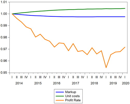
Even if the results found thus far seem to be sufficient to answer the question of the underlying demand and growth regimes of the Danish economy, the use of an empirical SFC model provides us with more information that allows us to dig deeper into them. In Figure A3, we show the trajectories of the markup, unit costs, and the profit rate (defined as the ratio of profits to the stock of capital in the previous period). Each of these three variables seem to follow a reasonable path after the economy is hit by the shock. As shown in the theoretical section, the fall of the markup should go hand in hand with the drop in the profit share, which is indeed what is observed in the figure. Unit costs, for their part, increase in line with the upward movement of real wages shown in Figure A4. As a consequence of higher unit costs and a lower markup, the profit rate is negatively affected, ending up approximately 3% lower than its baseline value in the long run.

In Figure A4, we plot the main drivers of private consumption, the engine of a wage-led economy. As mentioned before, the real wage is positively affected by an increase in the bargaining power of workers. Real disposable income therefore also increases, though to a lesser extent than its other components (such as capital (property) income and taxes) have not been shocked. The other driver of consumption is financial net wealth, which also goes up as the increase in households’ income leads to an increase in savings, resulting over time in a higher stock of wealth. Given the nature of the shock, the latter effect is of course smaller than the one found on real wages and disposable income, but still plays a role. This is an example of the type of dynamic feedback effects that SFC models can capture, thereby enriching the analysis. Finally, it is found that in the long run, employment is slightly lower than in the baseline, the reason being the mild decrease in real GDP. However, the fall in employment is not sufficient to undermine the positive effect that higher real wages have on disposable income. Had the investment been more sensitive to the distributive shock, it could perhaps have been the case that demand and employment fall to such an extent that disposable income is not strong enough to stimulate consumption. That is presumably what a fully-fledged profit-led economy would look like, but according to the results of this analysis Denmark does not fall in that category.

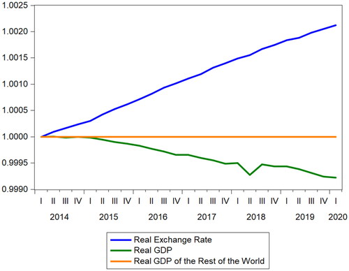
Finally, we explore the evolution of the determinants of trade flows. Even if these flows do not seem to be driving the results, it is worth examining if their behavior is in line with the underlying theory. In Figure A2, we found that both exports and imports fall in the long run, though by negligible values. The common determinant of trade flows is the real exchange rate, which was defined as the ratio of domestic prices to foreign prices. Figure A5 shows that a more progressive income distribution results in a real exchange rate appreciation, which is in line with the neo-Kaleckian theory of demand and income distribution in open economies. More specifically, higher nominal wages imply increases in domestic prices (albeit lower ones, so that real wages increase) which, given the nominal exchange rate and foreign prices, lead to an increase in the real exchange rate. For a given level of activity of trading partners, a more appreciated real exchange rate reduces exports, as shown in Figure A2. In the case of imports, the real exchange rate appreciation acts as a stimulant, but the overall effect ends up being negative because of the fall in economic activity over time (the equation can be found in the annex).

Discussion

Based on the results presented above, we find that Denmark cannot be unequivocally categorized as either wage-led or profit-led. While the demand regime seems to be weakly wage-led (at least in the medium to long term), the growth regime was found to be profit-led. An increase in the wage share is associated with an increase in capacity utilization, not because of an overall positive effect on aggregate demand but due to a lower accumulation of capital. From a theoretical point of view, the effects of an increase in the wage share on both investment and consumption are in line with our predictions. Net exports are affected positively by the increase in the wage share, which is explained by the fact that exports fall mildly following a real exchange rate appreciation, whereas imports fall more strongly, in line with the evolution of domestic activity. The overall effect on the aggregated demand, however, is almost negligible as can be seen in Figure A2 and Figure A5.

If we compare the overall result with the existing literature, our findings do not fully support either the conclusions obtained by Onaran and Obst (2016) and Oyvat, Öztunalı, and Elgin (2020) whereby the Danish economy is profit-led, nor the ones from Obst, Onaran, and Nikolaidi (2017) and Storm and Naastepad (2012) stating that Denmark is wage-led. Rather, our findings seem closer to the ones obtained by Bengtsson and Stockhammer (2021), who characterize Denmark as weakly wage-led.

Our approach tries to accommodate some of the weaknesses identified especially in the “structural approach” in three specific areas. Firstly, instead of focusing purely on flows, we have introduced stock variables (both financial and fixed capital) to the analysis. We find that stock-flow interactions considerably enrich the analysis. For example, the decision to invest and consume affects both financial and non-financial stocks associated with households and firms, and the resulting changes in these stocks feed back into consumption and investment. The relevance of including stock variables is also clearly seen in Figure A4, where the effect of the shock via consumption channel is determined by both an increase in real disposable income and real financial net wealth.

Secondly, endogenizing income distribution makes it possible to not only capture the effects of income shares on demand but the vice versa as well. This can be seen in Figure A1, where the profit share keeps changing throughout the simulation period, which provides a better understanding of the bi-directional causality between income distribution and aggregate demand, beyond the one-way relationship that characterizes the existing studies. Finally, since Denmark can be described as a mature economy with a very low level of unemployment, changes in the rate of unemployment are expected to affect wage-setting decisions and thereby prices and aggregate demand. In this regard, Figure A4, shows that the level of employment is negatively affected by the shock because of the fall in overall domestic economic activity, which partly outweighs the effect on disposable income earned by households as a result of the increase in the real wage rate.

Adding these three elements to the analysis therefore clearly improves the understanding of the effect of changes in income distribution on the rest of the economy. Taking this value-added into account, we return to our original question: can the Danish economy be unequivocally classified as either profit-led or wage-led?

The answer to this question is both yes and no. In the case of the analysis, the answer would lean toward what Hein (2014) identifies as an intermediate regime, where the demand is wage-led and the accumulation is profit-led. However, the effect in the very short-run seems to be neutral, as the overall effect on GDP is almost negligible. Furthermore, although our approach seems to have improved the understanding of the link between income distribution and aggregate demand, further investigation still needs to take place to provide a more precise characterization of the Danish economy. As presented in both Blecker (2016) and Skott (2017), the nature of the shock should be identified and discussed as well, since different shocks might affect not only the wage share but also other variables differently, which might cause a shift in the demand regime from wage-led to profit-led or the other way around.¹⁸

Despite the possible loss of generality discussed above, our results still seem to suggest, that the approach used in this article has the potential to contribute to the literature on how to identify the underlying demand and growth regimes of a given economy.

Conclusions

Developing ways of assessing the wage-led or profit-led nature of an economy has become a popular research area within the Post-Keynesian literature. So far, two empirical strategies have been followed to identify the underlying demand regime, the so-called “structural” approach, in which each component of aggregate demand is estimated individually, and the “aggregative” approach which consists of a single econometric estimation of aggregate demand on the wage share and a set of control variables related to the individual components of aggregate demand. In this paper, we harness the advantages of empirical stock-flow consistent models and utilize it to address the dichotomy between wage-led and profit-led regimes. This approach combines the strengths of the two other approaches: (i) the detailed description of the diversity of transactions embedded in the economy retains the advantage of the “structural” approach, even enhancing it through the wide range of processes modeled beyond the aggregate demand equations, and (ii) even if we estimate each equation separately, the model variables can affect each other in such a way that the dynamic effects captured in the “aggregative” approach are present. Furthermore, we accommodate the critique of the two existing empirical approaches by integrating three important aspects in our approach: (i) including stocks in the analysis (both financial and fixed assets), (ii) endogenizing the income distribution, which allows for multiple feedback mechanisms to play out in the model dynamics, and (iii) including the labor market in the analysis. Using this SFC approach we build an empirical model for the Danish economy for the period 2005–2020 in order to discuss whether the Danish economy is profit-led or wage-led.

To explore the interaction between income distribution and aggregate demand, we introduced a shock in the model, whereby we increased the labor income share. We found that over time this had a positive effect on capacity utilization and a negative impact on the rate of accumulation. The negative effect of a more progressive income distribution on investment reduced both the aggregate demand and the stock of fixed capital. Over time, the drop in the stock of fixed capital exceeded the drop in GDP, resulting in an increase in the rate of capacity utilization. This result might misleadingly lead to the conclusion that demand in the Danish economy is wage-led, whereas we actually observed a mild negative impact on real GDP. Thus, based on our findings, a case can be made that Denmark can neither be characterized as purely profit-led nor wage-led, at least during the period 2005–2020. One could argue that providing a more conclusive answer on the underlying demand regime would require a more fundamental understanding on how different shocks affect the economy and what are the main transmission channels that explain the results. The approach used in this paper provides a basis for this kind of analysis that can be useful in uncovering more insights into this topic. However, it should be noted that building an empirical SFC model is significantly more time-consuming than the other structural and the aggregative approaches, a non-negligible variable that needs to be accounted for when defining a research strategy.

Disclosure statement

No potential conflict of interest was reported by the author(s).

Additional information

Notes on contributors

Mikael Randrup Byrialsen

Mikael Randrup Byrialsen, Sebastian Valdecantos, Hamid Raza, and Thibault Laurentjoye are at MaMTEP, Aalborg University Business School, Aalborg, Denmark.

Sebastian Valdecantos

Mikael Randrup Byrialsen, Sebastian Valdecantos, Hamid Raza, and Thibault Laurentjoye are at MaMTEP, Aalborg University Business School, Aalborg, Denmark.

Hamid Raza

Mikael Randrup Byrialsen, Sebastian Valdecantos, Hamid Raza, and Thibault Laurentjoye are at MaMTEP, Aalborg University Business School, Aalborg, Denmark.

Thibault Laurentjoye

Mikael Randrup Byrialsen, Sebastian Valdecantos, Hamid Raza, and Thibault Laurentjoye are at MaMTEP, Aalborg University Business School, Aalborg, Denmark.

Notes

1 Recent examples of empirical analyses using the structural approach are Onaran and Obst (2016) for 15 European countries estimated individually, and Stockhammer and Wildauer (2016) who estimate this relationship for a panel of 18 OECD countries.

2 Recent examples of analyses undertaken through the aggregative approach are Charpe, Bridji, and McAdam (2020) for the UK, the US and France, and Santos & Araujo (2018) for the US.

3 Even if some stock-flow relations can be included in single-equation estimation methods (like wealth in the consumption function), the dynamics captured by the model would not be exhastive as in a structural macroeconometric model, as the causality would only run in one direction (from wealth to consumption, but not from consumption to wealth).

4 For a more detailed discussion see Blecker (2016).

5 To avoid simultaneity biases, lags of the endogenous variables can be used.

6 The stability condition states that savings are more elastic towards changes in the endogenous variables than the sum of investment, the budget deficit, and net exports.

7 The inclusion of net exports tends to reduce the likelihood of economies being wage-led, as higher real wages are associated with a loss of competitiveness, as shown in Equation (6)(6) $$b={\mathit{\text{nx}}}_1\mathrm{*}\mathit{\text{rer}}\left(\pi \right)+{\mathit{\text{nx}}}_2\mathrm{*}{u}_f-{\mathit{\text{nx}}}_3\mathrm{*}u+\mathit{\text{rca}}$$(6) .

8 A more detailed presentation of the data and assumptions used in the model used can be found in Byrialsen, Raza, and Valdecantos (2022).

9 The results of the estimations together with the overall performance of the model at fitting the actual data can be found in Byrialsen, Raza, and Valdecantos (2022) or upon request to the author.

10 Endogenizing these processes requires an explicit investigation of the entire financial market, which would be beyond the scope of this paper.

11 Despite the assumption, that all production takes place in the sector for non-financial corporation, gross operating surplus is still distributed to the domestic sectors to establish the same income flows as reported in the national account. These flows are kept as exogenous shares of the total gross operating surplus in the model.

12 The model used to address the question of this paper differs from the benchmark and other applications like Raza et al. (2023) and Byrialsen, Raza, and Valdecantos (2024) in a number of ways. In the case of Raza et al. (2023), where the focus is on inflation, there is a more detailed specification of price indices and also how different tax rates can affect price dynamics following a supply side shock. These elements are included in the case of Byrialsen, Raza, and Valdecantos (2024), to which non-linearities are included in some behavioral equations to improve the accuracy and precision of the estimations. The model used in this paper is simpler compared to the previously mentioned.

13 Each country’s real GDP was converted into USD and weighted by its share on Danish export basket.

14 The real exchange rate index was built as the weighted average of the bilateral real exchange rate, which was in turn computed using consumer price indices and nominal exchange rates.

15 As done by Blecker (2016), when referring to the long run effects of a specific shock we are not appealing to the neoclassical conception of the long run or steady state in the neoclassical sense, where all variables grow at the same rate, or to the theoretical notion of the long period made by the classics, where variables rest at their “normal” rates. The concept “long term” is used here in the spirit of Kalecki’s view that “the long-run trend is but a slowly changing component of a chain of short-period situations; it has no independent entity” (Kalecki 1971, 165).

16 While the gross fixed capital formation was 20% of aggregate demand in 2014, private consumption was 47%.

17 Defining the rate of capacity utilization as $u=\frac{y}{y^{\mathit{\text{fc}}}},$ and full capacity output as $y^{\mathit{\text{fc}}}=K_{t-1}/v,$ with v being a technologically determined capital-potential output ratio, if k falls more than y then u will increase.

18 Since the purpose of this article is to present a third approach to the identification of whether an economy can be characterized as wage-led or profit-led, the discussion of the nature of different shocks is beyond the scope of this paper.

19 Each country’s real GDP was converted into USD and weighted by its share on Danish export basket.

20 The real exchange rate index was built as the weighted average of the bilateral real exchange rate, which was in turn computed using consumer price indices and nominal exchange rates.

Appendices Appendix A.

 Figures

 

Figure A1. Impact of stronger unions on income distribution, utilization and accumulation.

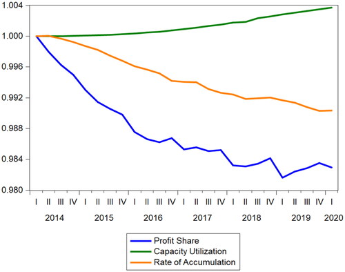
Figure A2. Impact of stronger unions on aggregate demand.

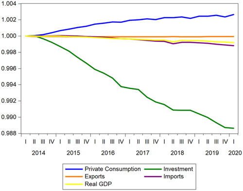
Figure A3. Impact of stronger unions on the determinants of NFC’s investment.

Source: self-elaborated

Figure A4. Impact of stronger unions on the determinants of Households’ consumption.

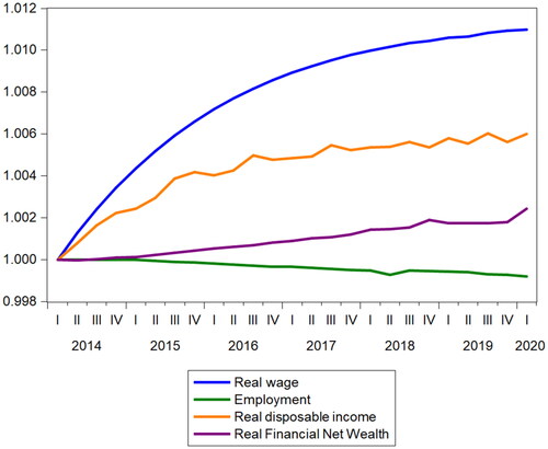
Figure A5. Impact of stronger unions on the determinants of foreign trade.

Appendix B.

 Equilibrium rates and derivatives

The equilibrium current account balance (scaled by the nominal capital stock) is obtained by inserting the expression for $u^{\mathrm{*}}$ in Equation (6). (B1) $$b^{\mathrm{*}}=\frac{\begin{array}{c}\left[{\mathit{\text{nx}}}_1\mathrm{\hspace{0.17em}}\mathrm{*}\mathrm{\hspace{0.17em}}\mathit{\text{rer}}+{\mathit{\text{nx}}}_2{u}_f+\mathit{\text{rca}}\right]⟨\pi \left[s_{\mathit{\Pi }}\left(1-{\theta }_{\mathit{\Pi }}\right)+s_W\left({\theta }_W-1\right)+{\theta }_W-{\theta }_{\mathit{\Pi }}\right]+s_W\left({1-\theta }_W\right)-{\theta }_W\\ +v\left({\mathit{\text{nx}}}_3-i_2\right)⟩-{\mathit{\text{nx}}}_{3}v\left\{i_0+i_1\pi +i_{3}q{+\mathit{\text{nx}}}_1\mathrm{\hspace{0.17em}}\mathrm{*}\mathrm{\hspace{0.17em}}\mathit{\text{rer}}+{\mathit{\text{nx}}}_2\mathrm{\hspace{0.17em}}\mathrm{*}\mathrm{\hspace{0.17em}}{u}_f+z+\mathit{\text{ra}}\left(1-{\theta }_{\mathit{\Pi }}\right)\left(1-s_{\mathit{\Pi }}\right)\right\}\end{array}}{\pi \left[s_{\mathit{\Pi }}\left(1-{\theta }_{\mathit{\Pi }}\right)+s_W\left({\theta }_W-1\right)+{\theta }_W-{\theta }_{\mathit{\Pi }}\right]+s_W\left({1-\theta }_W\right)-{\theta }_W+v\left({\mathit{\text{nx}}}_3-i_2\right)}$$(B1)

The equilibrium budget deficit is obtained by plugging $u^{\mathrm{*}}$ in Equation (9). (B2) $$d^{\mathrm{*}}=\frac{\begin{array}{c}\left\{i_0+i_1\pi +i_{3}q{+\mathit{\text{nx}}}_1\mathrm{\hspace{0.17em}}\mathrm{*}\mathrm{\hspace{0.17em}}\mathit{\text{rer}}+{\mathit{\text{nx}}}_2\mathrm{\hspace{0.17em}}\mathrm{*}\mathrm{\hspace{0.17em}}{u}_f+z+\mathit{\text{ra}}\left(1-{\theta }_{\mathit{\Pi }}\right)\left(1-s_{\mathit{\Pi }}\right)\right\}\left[{\theta }_W\left(\pi -1\right)-{\theta }_{\mathit{\Pi }}\pi \right]\\ +\left\{\pi \left[s_{\mathit{\Pi }}\left(1-{\theta }_{\mathit{\Pi }}\right)+s_W\left({\theta }_W-1\right)+{\theta }_W-{\theta }_{\mathit{\Pi }}\right]+s_W\left({1-\theta }_W\right)-{\theta }_W+v\left({\mathit{\text{nx}}}_3-i_2\right)\}\right[\mathit{\text{ra}}\left[\left(1-c\right)-{\theta }_{\mathit{\Pi }}\right]+z]\hfill \end{array}}{\pi \left[s_{\mathit{\Pi }}\left(1-{\theta }_{\mathit{\Pi }}\right)+s_W\left({\theta }_W-1\right)+{\theta }_W-{\theta }_{\mathit{\Pi }}\right]+s_W\left({1-\theta }_W\right)-{\theta }_W+v\left({\mathit{\text{nx}}}_3-i_2\right)}$$(B2)

Partial derivatives for $u^{\mathrm{*}},$ $g^{\mathrm{*}},$ $b^{\mathrm{*}}$ and $d^{\mathrm{*}}:$ (B3) $$\frac{\partial u^{\mathrm{*}}}{\partial \pi }=\frac{\begin{array}{c}v{i}_1⟨\pi \left[s_{\mathit{\Pi }}\left(1-{\theta }_{\mathit{\Pi }}\right)+s_W\left({\theta }_W-1\right)+{\theta }_W-{\theta }_{\mathit{\Pi }}\right]+s_W\left({1-\theta }_W\right)-{\theta }_W+v\left({\mathit{\text{nx}}}_3-i_2\right)⟩\hfill \\ -v\{i_0+i_1\pi +i_{3}q{+\mathit{\text{nx}}}_1\mathrm{\hspace{0.17em}}\mathrm{*}\mathrm{\hspace{0.17em}}\mathit{\text{rer}}+{\mathit{\text{nx}}}_2\mathrm{\hspace{0.17em}}\mathrm{*}\mathrm{\hspace{0.17em}}{u}_f+z+\mathit{\text{ra}}\left(1-{\theta }_{\mathit{\Pi }}\right)\left(1-s_{\mathit{\Pi }}\right)\}\\ \left[s_{\mathit{\Pi }}\left(1-{\theta }_{\mathit{\Pi }}\right)+s_W\left({\theta }_W-1\right)+{\theta }_W-{\theta }_{\mathit{\Pi }}\right]\end{array}}{{⟨\pi \left[s_{\mathit{\Pi }}\left(1-{\theta }_{\mathit{\Pi }}\right)+s_W\left({\theta }_W-1\right)+{\theta }_W-{\theta }_{\mathit{\Pi }}\right]+s_W\left({1-\theta }_W\right)-{\theta }_W+v\left({\mathit{\text{nx}}}_3-i_2\right)⟩}^2}$$(B3) (B4) $$\frac{\partial g^{\mathrm{*}}}{\partial \pi }=\frac{\begin{array}{l}\{\left[s_{\mathit{\Pi }}\left(1-{\theta }_{\mathit{\Pi }}\right)+s_W\left({\theta }_W-1\right)+{\theta }_W-{\theta }_{\mathit{\Pi }}\right]\left[i_0+{2i}_1\pi +i_{3}q\right]\\ +i_1\left[s_W\left({1-\theta }_W\right)-{\theta }_W+v\left({\mathit{\text{nx}}}_3-i_2\right)\right]\}[\pi \left[s_{\mathit{\Pi }}\left(1-{\theta }_{\mathit{\Pi }}\right)+s_W\left({\theta }_W-1\right)+{\theta }_W-{\theta }_{\mathit{\Pi }}\right]\\ +s_W\left({1-\theta }_W\right)-{\theta }_W+v\left({\mathit{\text{nx}}}_3-i_2\right)]\end{array}}{{⟨\pi \left[s_{\mathit{\Pi }}\left(1-{\theta }_{\mathit{\Pi }}\right)+s_W\left({\theta }_W-1\right)+{\theta }_W-{\theta }_{\mathit{\Pi }}\right]+s_W\left({1-\theta }_W\right)-{\theta }_W+v\left({\mathit{\text{nx}}}_3-i_2\right)⟩}^2}-\frac{-\left\{\left[i_0+i_1\pi +i_{3}q\right]⟨\pi \left[s_{\mathit{\Pi }}\left(1-{\theta }_{\mathit{\Pi }}\right)+s_W\left({\theta }_W-1\right)+{\theta }_W-{\theta }_{\mathit{\Pi }}\right]+s_W\left({1-\theta }_W\right)-{\theta }_W+v\left({\mathit{\text{nx}}}_3-i_2\right)⟩\right\}}{{⟨\pi \left[s_{\mathit{\Pi }}\left(1-{\theta }_{\mathit{\Pi }}\right)+s_W\left({\theta }_W-1\right)+{\theta }_W-{\theta }_{\mathit{\Pi }}\right]+s_W\left({1-\theta }_W\right)-{\theta }_W+v\left({\mathit{\text{nx}}}_3-i_2\right)⟩}^2}+\frac{+i_{2}v\left[{\mathit{\text{nx}}}_1\mathrm{\hspace{0.17em}}\mathrm{*}\mathrm{\hspace{0.17em}}\mathit{\text{rer}}+{\mathit{\text{nx}}}_2\mathrm{\hspace{0.17em}}\mathrm{*}\mathrm{\hspace{0.17em}}{u}_f+z+\mathit{\text{ra}}\left(1-{\theta }_{\mathit{\Pi }}\right)\left(1-s_{\mathit{\Pi }}\right)\right]\left[s_{\mathit{\Pi }}\left(1-{\theta }_{\mathit{\Pi }}\right)+s_W\left({\theta }_W-1\right)+{\theta }_W-{\theta }_{\mathit{\Pi }}\right]}{{⟨\pi \left[s_{\mathit{\Pi }}\left(1-{\theta }_{\mathit{\Pi }}\right)+s_W\left({\theta }_W-1\right)+{\theta }_W-{\theta }_{\mathit{\Pi }}\right]+s_W\left({1-\theta }_W\right)-{\theta }_W+v\left({\mathit{\text{nx}}}_3-i_2\right)⟩}^2}$$(B4) (B5) $$\frac{\partial b^{\mathrm{*}}}{\partial \pi }=\frac{\begin{array}{l}(\left[{\mathit{\text{nx}}}_1\mathrm{\hspace{0.17em}}\mathrm{*}\mathrm{\hspace{0.17em}}\mathit{\text{rer}}+{\mathit{\text{nx}}}_2{u}_f+\mathit{\text{rca}}\right]\left[s_{\mathit{\Pi }}\left(1-{\theta }_{\mathit{\Pi }}\right)+s_W\left({\theta }_W-1\right)+{\theta }_W-{\theta }_{\mathit{\Pi }}\right]-{\mathit{\text{nx}}}_{3}v{i}_1)-[{\mathit{\text{nx}}}_1\mathrm{\hspace{0.17em}}\mathrm{*}\mathrm{\hspace{0.17em}}\mathit{\text{rer}}+{\mathit{\text{nx}}}_2{u}_f+\mathit{\text{rca}}]\\ 〈\pi \left[s_{\mathit{\Pi }}\left(1-{\theta }_{\mathit{\Pi }}\right)+s_W\left({\theta }_W-1\right)+{\theta }_W-{\theta }_{\mathit{\Pi }}\right]+s_W\left({1-\theta }_W\right)-{\theta }_W+v\left({\mathit{\text{nx}}}_3-i_2\right)〉-{\mathit{\text{nx}}}_{3}u\mathrm{*}(s_{\mathit{\Pi }}\left(1-{\theta }_{\mathit{\Pi }}\right)+s_W\left({\theta }_W-1\right)+{\theta }_W-{\theta }_{\mathit{\Pi }})\end{array}}{\pi \left[s_{\mathit{\Pi }}\left(1-{\theta }_{\mathit{\Pi }}\right)+s_W\left({\theta }_W-1\right)+{\theta }_W-{\theta }_{\mathit{\Pi }}\right]+s_W\left({1-\theta }_W\right)-{\theta }_W+v\left({\mathit{\text{nx}}}_3-i_2\right)}$$(B5) (B6) $$\frac{\partial d^{\mathrm{*}}}{\partial \pi }=\frac{\begin{array}{c}(\{i_0+2i_1\pi +i_{3}q{+\mathit{\text{nx}}}_1\mathrm{*}\mathit{\text{rer}}+{\mathit{\text{nx}}}_2\mathrm{*}{u}_f+z+\mathit{\text{ra}}\left(1-{\theta }_{\Pi }\right)\left(1-s_{\Pi }\right)\}\left[{\theta }_W-{\theta }_{\Pi }\right]+\{s_{\Pi }\left(1-{\theta }_{\Pi }\right)+s_W\left({\theta }_W-1\right)+{\theta }_W-{\theta }_{\Pi }\})\\ -(\frac{\mathrm{u}}{v}\left[{\theta }_W\left(\pi -1\right)-{\theta }_{\Pi }\pi \right]+\{\pi \left[s_{\Pi }\left(1-{\theta }_{\Pi }\right)+s_W\left({\theta }_W-1\right)+{\theta }_W-{\theta }_{\Pi }\right]+s_W\left({1-\theta }_W\right)-{\theta }_W+v({\mathit{\text{nx}}}_3-i_2)\}[\mathit{\text{ra}}[\left(1-c\right)-{\theta }_{\Pi }]+z])\\ \mathrm{*}\left[s_{\Pi }\left(1-{\theta }_{\Pi }\right)+s_W\left({\theta }_W-1\right)+{\theta }_W-{\theta }_{\Pi }\right]\end{array}}{\pi \left[s_{\Pi }\left(1-{\theta }_{\Pi }\right)+s_W\left({\theta }_W-1\right)+{\theta }_W-{\theta }_{\Pi }\right]+s_W\left({1-\theta }_W\right)-{\theta }_W+v\left({\mathit{\text{nx}}}_3-i_2\right)}$$(B6)

Appendix C.

 Balance sheet (Table C1) and transactions flow matrix (Table C2)

 

Table C1. Financial balance sheet for Denmark – ‘+’ expresses an asset, while ‘-‘ is associated with a liability.

	Households	Non-financial corporations	Financial corporations	General Government	Rest of the world	Total
Interest Bearing Assets	${+\mathit{\text{IBA}}}_t^H$	${+\mathit{\text{IBA}}}_t^N$	${-\mathit{\text{IBA}}}_t^F$	${+\mathit{\text{IBA}}}_t^G$	${+\mathit{\text{IBA}}}_t^W$	0
Equities	${+\mathit{\text{EQ}}}_t^H$	${-\mathit{\text{EQ}}}_t^N$	${-\mathit{\text{EQ}}}_t^F$	$+{\mathit{\text{EQ}}}_t^G$	${-\mathit{\text{EQ}}}_t^W$	0
Securities	${+\mathit{\text{SEC}}}_t^H$	${-\mathit{\text{SEC}}}_t^N$	${+\mathit{\text{SEC}}}_t^F$	${-\mathit{\text{SEC}}}_t^G$	${+\mathit{\text{SEC}}}_t^W$	0
Insurance	$+{\mathit{\text{INS}}}_t^H$	$0$	$-{\mathit{\text{INS}}}_t^F$	$0$	${+\mathit{\text{INS}}}_t^W$	0
Loans	${-L}_t^H$	${-L}_t^N$	${+L}_t^F$	${-L}_t^G$	${-L}_t^W$	0
Net worth	$W_t^H$	$W_t^N$	$W_t^F$	$W_t^G$	$W_t^W$	0

Table C2. Transaction flow matrix for Denmark – ‘-’ is associated with an outflow of the sector.

	Households		Non-financial corporations		Financial corporations		General Government		Rest of the world		Total
	Current	Capital	Current	Capital	Current	Capital	Current	Capital	Current	Capital
Private consumption	$-C_t$		$C_t$								0
Investment (Buildings and Dw)		$-I_{\mathit{\text{BDt}}}^H$	$I_{\mathit{\text{BDt}}}^{}$	$-I_{\mathit{\text{BDt}}}^N$		$-I_{\mathit{\text{BDt}}}^F$		$-I_{\mathit{\text{BDt}}}^G$			0
Investment (Equipment)		$-I_{\mathit{\text{Et}}}^H$	$I_{\mathit{\text{Et}}}^{}$	$-I_{\mathit{\text{Et}}}^N$		$-I_{\mathit{\text{Et}}}^F$		$-I_{\mathit{\text{Et}}}^G$			0
Investment (Inventories)			$I_{\mathit{\text{INVt}}}^{}$	$-I_{\mathit{\text{INVt}}}^N$
Government consumption			$G_t$				$-G_t$				0
Net export			${\mathit{\text{NX}}}_t$						$-{\mathit{\text{NX}}}_t$		0
Wage Bill	${\mathit{\text{WB}}}_t^H$		$-{\mathit{\text{WB}}}_t^{}$						${\mathit{\text{WB}}}_t^W$		0
Gross Operating Surplus	${\mathit{\text{GOS}}}_t^H$		${\mathit{\text{GOS}}}_t^N$		${\mathit{\text{GOS}}}_t^F$		${\mathit{\text{GOS}}}_t^G$				0
Net indirect Taxes			${-\mathit{\text{NIT}}}_t^N$				${\mathit{\text{NIT}}}_t^G$		$-{\mathit{\text{NIT}}}_t^W$		0
Net Interest on Assets	${\mathit{\text{NIA}}}_t^H$		${\mathit{\text{NIA}}}_t^N$		${\mathit{\text{NIA}}}_t^F$		${\mathit{\text{NIA}}}_t^G$		${\mathit{\text{NIA}}}_t^W$		0
Net Income on Insurance	${\mathit{\text{NII}}}_t^H$		${\mathit{\text{NII}}}_t^N$		${\mathit{\text{NII}}}_t^F$		${\mathit{\text{NII}}}_t^G$		${\mathit{\text{NII}}}_t^W$		0
Net dividends	${\mathit{\text{ND}}}_t^H$		${\mathit{\text{ND}}}_t^N$		${\mathit{\text{ND}}}_t^F$		${\mathit{\text{ND}}}_t^G$		${\mathit{\text{ND}}}_t^W$		0
Directs Taxes	${-\mathit{\text{DT}}}_t^H$		${-\mathit{\text{DT}}}_t^N$		${-\mathit{\text{DT}}}_t^F$		${\mathit{\text{DT}}}_t^G$		${-\mathit{\text{DT}}}_t^W$		0
Social Contributions	${-\mathit{\text{SC}}}_t^H$				${\mathit{\text{SC}}}_t^F$		${\mathit{\text{SC}}}_t^G$		${\mathit{\text{SC}}}_t^W$		0
Social Benefits	${\mathit{\text{SB}}}_t^H$				${-\mathit{\text{SB}}}_t^F$		${-\mathit{\text{SB}}}_t^G$		${\mathit{\text{SB}}}_t^W$		0
Other current Transfers	${\mathit{\text{OCT}}}_t^H$		${-\mathit{\text{OCT}}}_t^N$		${\mathit{\text{OCT}}}_t^F$		${-\mathit{\text{OCT}}}_t^G$		${\mathit{\text{OCT}}}_t^W$		0
Savings/current account	${-S}_t^H$	$S_t^H$	${-S}_t^N$	$S_t^N$	${-S}_t^F$	$S_t^F$	$-S_t^G$	$S_t^G$	$-{\mathit{\text{CA}}}_t^{}$	${\mathit{\text{CA}}}_t^{}$	0
Capital Transfers		${\mathit{\text{KT}}}_t^H$		${\mathit{\text{KT}}}_t^N$		${-\mathit{\text{KT}}}_t^F$		${-\mathit{\text{KT}}}_t^G$		${-\mathit{\text{KT}}}_t^W$	0
Others		${-\mathit{\text{NP}}}_t^H$		${-\mathit{\text{NP}}}_t^N$				${\mathit{\text{NP}}}_t^G$		${\mathit{\text{NP}}}_t^W$	0
Net Lending		${\mathit{\text{NL}}}_t^H$		${\mathit{\text{NL}}}_t^N$		${\mathit{\text{NL}}}_t^F$		${\mathit{\text{NL}}}_t^G$		${\mathit{\text{NL}}}_t^W$	0
Adjustment		${\mathit{\text{adj}}}_t^H$		${\mathit{\text{adj}}}_t^N$		${\mathit{\text{adj}}}_t^F$		${\mathit{\text{adj}}}_t^G$		${\mathit{\text{adj}}}_t^W$	0
Δ Interest Bearing Assets		${-\Delta \mathit{\text{IBA}}}_t^H$		${-\Delta \mathit{\text{IBA}}}_t^N$		${\Delta \mathit{\text{IBA}}}_t^F$		${-\Delta \mathit{\text{IBA}}}_t^G$		${-\Delta \mathit{\text{IBA}}}_t^W$	0
Δ Equities		${-\Delta \mathit{\text{EQ}}}_t^H$		${\Delta \mathit{\text{EQ}}}_t^N$		${-\Delta \mathit{\text{EQ}}}_t^F$		${-\Delta \mathit{\text{EQ}}}_t^G$		${\Delta \mathit{\text{EQ}}}_t^W$	0
Δ Securities		${-\Delta \mathit{\text{SEC}}}_t^H$		${\Delta \mathit{\text{SEC}}}_t^N$		${-\Delta \mathit{\text{SEC}}}_t^F$		${\Delta \mathit{\text{SEC}}}_t^G$		${-\Delta \mathit{\text{SEC}}}_t^W$	0
Δ Insurance		${-\Delta \mathit{\text{INS}}}_t^H$		${-\Delta \mathit{\text{INS}}}_t^N$		$\Delta {\mathit{\text{INS}}}_t^F$		${-\Delta \mathit{\text{INS}}}_t^G$		${-\Delta \mathit{\text{INS}}}_t^W$	0
Δ Loans		${\Delta L}_t^H$		${\Delta L}_t^N$		${-\Delta L}_t^F$		${\Delta L}_t^G$		${\Delta L}_t^W$	0
Rev. Interest Bearing Assets		${-\mathit{\text{rev}}}_{\mathit{\text{IBA}}}^H$		${-\mathit{\text{rev}}}_{\mathit{\text{IBA}}}^N$		${\mathit{\text{rev}}}_{\mathit{\text{IBA}}}^F$		${-\mathit{\text{rev}}}_{\mathit{\text{IBA}}}^G$		${-\mathit{\text{rev}}}_{\mathit{\text{IBA}}}^W$	0
Rev. Equities		${-\mathit{\text{rev}}}_{\mathit{\text{EQ}}}^H$		${\mathit{\text{rev}}}_{\mathit{\text{EQ}}}^N$		${-\mathit{\text{rev}}}_{\mathit{\text{EQ}}}^F$		${-\mathit{\text{rev}}}_{\mathit{\text{EQ}}}^G$		${\mathit{\text{rev}}}_{\mathit{\text{EQ}}}^W$	0
Rev. Securities		${-\mathit{\text{rev}}}_{\mathit{\text{SEC}}}^H$		${\mathit{\text{rev}}}_{\mathit{\text{SEC}}}^N$		$-{\mathit{\text{rev}}}_{\mathit{\text{SEC}}}^F$		${\mathit{\text{rev}}}_{\mathit{\text{SEC}}}^G$		${-\mathit{\text{rev}}}_{\mathit{\text{SEC}}}^W$	0
Rev. Insurance		${-\mathit{\text{rev}}}_{\mathit{\text{INS}}}^H$		${-\mathit{\text{rev}}}_{\mathit{\text{INS}}}^N$		${\mathit{\text{rev}}}_{\mathit{\text{INS}}}^F$		${-\mathit{\text{rev}}}_{\mathit{\text{INS}}}^G$		${-\mathit{\text{rev}}}_{\mathit{\text{INS}}}^W$	0
Rev. Loans		${\mathit{\text{rev}}}_L^H$		${\mathit{\text{rev}}}_L^N$		${-\mathit{\text{rev}}}_L^F$		${\mathit{\text{rev}}}_L^G$		${\mathit{\text{rev}}}_L^W$	0
Rev. Building and Dwellings		$-{\mathit{\text{rev}}}_{\mathit{\text{BD}}}^H$		$-{\mathit{\text{rev}}}_{\mathit{\text{BD}}}^N$		$-{\mathit{\text{rev}}}_{\mathit{\text{BD}}}^F$		$-{\mathit{\text{rev}}}_{\mathit{\text{BD}}}^G$			0
Rev. Equipment		$-{\mathit{\text{rev}}}_E^H$		$-{\mathit{\text{rev}}}_E^N$		$-{\mathit{\text{rev}}}_E^F$		$-{\mathit{\text{rev}}}_E^G$			0
Δ Net worth		${-\Delta W}_t^H$		${-\Delta W}_t^N$		${-\Delta W}_t^F$		${-\Delta W}_t^G$		$\Delta \mathit{\text{NIIP}}$	0

Appendix D.

 Key drivers of the empirical SFC model for Denmark

To provide a clear flow of reading in the presentation of the main transmission channels presented in “Main transmission mechanisms” section, we have moved the more formal presentation of the key drivers of this dynamic to the appendix together with a discussion of the results of the estimations.

Households earn income from four sources: wages paid by firms ($W{B}^H$), gross operating surplus from production ($B_{2_t}^H$), net social transfers (${\mathit{\text{STR}}}^H$), and capital income (${\mathit{\text{Prop}}}_t^H$). (D1) $$Y_t^H=W{B}_t^H+{\mathit{\text{Prop}}}_t^H+B_{2_t}^H+{\mathit{\text{STR}}}_t^H$$(D1)

The wage bill is determined by the level of employment, which is given as the ratio of real production $y_t$ to productivity ($a$), times the endogenous wage rate. (D2) $$W{B}_t^H=\mathit{\text{wage}}\cdot N_t^H$$(D2)

Households’ consumption is a function of disposable income and a wealth. (D3) $$\Delta \mathrm{\text{ln}}\hspace{0.17em}\left(c_t\right)=1.58-0.33\mathrm{\hspace{0.17em}}\mathrm{*}\mathrm{\hspace{0.17em}}\mathit{\text{ln}}\left(c_{t-1}\right)+0.11\mathrm{\hspace{0.17em}}\mathrm{*}\mathrm{\hspace{0.17em}}\mathit{\text{ln}}\left(y{d}_{t-1}^1\right)+0.06\mathrm{\hspace{0.17em}}\mathrm{*}\mathrm{\hspace{0.17em}}\mathrm{\text{ln}}\hspace{0.17em}\left(y{d}_{t-1}^2\right)+0.03\mathrm{\hspace{0.17em}}\mathrm{*}\mathrm{\hspace{0.17em}}\mathit{\text{ln}}\left({\mathit{\text{fnw}}}_{t-1}\right)+0.06\mathrm{\hspace{0.17em}}\mathrm{*}\mathrm{\hspace{0.17em}}\Delta \mathrm{\text{ln}}\hspace{0.17em}\left({\mathit{\text{yd}}}_t^1\right)+0.06\mathrm{\hspace{0.17em}}\mathrm{*}\mathrm{\hspace{0.17em}}\Delta \mathrm{\text{ln}}\hspace{0.17em}\left({\mathit{\text{yd}}}_{t-2}^1\right)+0.09\mathrm{\hspace{0.17em}}\mathrm{*}\mathrm{\hspace{0.17em}}\Delta \mathrm{\text{ln}}\hspace{0.17em}\left({\mathit{\text{yd}}}_t^2\right)$$(D3)

In line with the underlying economic theory, there seems to be evidence of cointegration between real consumption and both real disposable income (of upper and lower classes) and real financial wealth. The consumption function is therefore estimated using an error correction model. It is seen from the expression that $0\le s_W<s_{\mathit{\Pi }}\le 1,$ which is in line with the theory.

The investment in equipment and machinery by non-financial corporations takes the following functional form: (D4) $$\Delta \mathit{\text{ln}}\left(\frac{i_{E,t}^N}{e_{t-1}^N}\right)=-0.01-0.17\mathrm{\hspace{0.17em}}\mathrm{*}\mathrm{\hspace{0.17em}}\Delta \mathit{\text{ln}}\left(\frac{i_{E_{t-1}}^N}{e_{t-2}^{\mathit{\text{NFC}}}}\right)+0.01\mathrm{\hspace{0.17em}}\mathrm{*}\mathrm{\hspace{0.17em}}\Delta \mathit{\text{ln}}\left({\mathrm{\pi }}_t\right)+0.32\mathrm{\hspace{0.17em}}\mathrm{*}\mathrm{\hspace{0.17em}}\Delta \mathit{\text{ln}}\mathrm{ }\left(u_t\right)-0.24\mathrm{\hspace{0.17em}}\mathrm{*}\mathrm{\hspace{0.17em}}\Delta \mathit{\text{ln}}\mathrm{ }\left(q_t\right)-0.41\mathrm{\hspace{0.17em}}\mathrm{*}\mathrm{\hspace{0.17em}}\mathit{\text{ln}}\left(\frac{i_{E_{t-1}}^N}{e_{t-2}^N}\right)+0.44\mathrm{\hspace{0.17em}}\mathrm{*}\mathrm{\hspace{0.17em}}\mathit{\text{ln}}\left({\mathrm{\pi }}_{t-1}\right)+0.49\mathrm{\hspace{0.17em}}\mathrm{*}\mathrm{\hspace{0.17em}}\mathit{\text{ln}}\left(u_{t-1}\right)+0.06\mathrm{\hspace{0.17em}}\mathrm{*}\mathrm{\hspace{0.17em}}\mathit{\text{ln}}\left(q_{t-1}\right)$$(D4)

The equation also includes a dummy variable to account for a few outliers that otherwise render the residuals non-normally distributed (see appendix for the full specification of the equation). The implicit long run coefficients are 1.07 for the profit share, 1.20 for the rate of capacity utilization, and 0.15 for Tobin’s “q”, also exhibiting a higher sensitivity of investment to “real” factors than financial ones. Unsurprisingly, the short run coefficients are smaller (though not statistically significant). Since we estimate the above equation as an error correction model, we find that the error correction coefficient is −0.41, which implies that the model will correct itself by 41 percent in every quarter and will thus quickly converge to a stable long-run relationship.

For the investment in buildings and dwellings by nonfinancial corporations, we obtained the following equation: (D5) $$\Delta \mathit{\text{ln}}\left(\frac{i_{\mathit{\text{BD}},t}^N}{{\mathit{\text{bd}}}_{t-1}^N}\right)=0.40-0.49\mathrm{\hspace{0.17em}}\mathrm{*}\mathrm{\hspace{0.17em}}\Delta \mathit{\text{ln}}\left(\frac{i_{{\mathit{\text{BD}}}_{t-1}}^N}{{\mathit{\text{bd}}}_{t-2}^N}\right)-0.09\mathrm{\hspace{0.17em}}\mathrm{*}\mathrm{\hspace{0.17em}}\Delta \mathit{\text{ln}}\left({\mathrm{\pi }}_t\right)+0.72\mathrm{\hspace{0.17em}}\mathrm{*}\mathrm{\hspace{0.17em}}\Delta \mathit{\text{ln}}\mathrm{ }\left(u_t\right)+0.01\mathrm{\hspace{0.17em}}\mathrm{*}\mathrm{\hspace{0.17em}}\Delta \mathit{\text{ln}}\mathrm{ }\left(q_t\right)-0.40\mathrm{\hspace{0.17em}}\mathrm{*}\mathrm{\hspace{0.17em}}\mathit{\text{ln}}\left(\frac{i_{{\mathit{\text{BD}}}_{t-1}}^N}{{\mathit{\text{bd}}}_{t-2}^N}\right)+0.40\mathrm{\hspace{0.17em}}\mathrm{*}\mathrm{\hspace{0.17em}}\Delta \mathit{\text{ln}}\left({\mathrm{\pi }}_{t-1}\right)+1.04\mathrm{\hspace{0.17em}}\mathrm{*}\mathrm{\hspace{0.17em}}\Delta \mathit{\text{ln}}\mathrm{ }\left(u_{t-1}\right)+0.09\mathrm{\hspace{0.17em}}\mathrm{*}\mathrm{\hspace{0.17em}}\Delta \mathit{\text{ln}}\mathrm{ }\left(q_{t-1}\right)$$(D5)

The long run coefficient defining the relationship between the profit share and the rate of accumulation of buildings and dwellings is 1.01, meaning that accumulation almost co-evolves one-for-one with income distribution. As shown in the equation, the short run effect is much lower (-0.09) and displays the “wrong” sign, though not statistically significant. Regarding the long run relationship between accumulation and capacity utilization, the coefficient is 2.6, signaling a high sensitivity of investment to the level of economic activity. The short run effect is smaller (0.72). Finally, the long run relationship between investment and Tobin’s “q” is estimated around 0.23, far below the impact of the other two determinants. The speed of adjustment toward the long-run relationship is 40 percent in every quarter (as the coefficient on the error term is −0.40). The complete estimation output can be found in the appendix.

As presented in “Main transmission mechanisms” section, investment in dwellings by households is a function of aggregate disposable income, the relative price of dwellings with respect to construction prices $\frac{P^{\mathit{\text{BD}}}}{P^I},$ and leverage. A significant long-run relationship is found between investment in buildings and dwellings and disposable income, relative prices, and households’ debt. The short-run effects exhibit signs in line with economic theory, although the coefficients of prices and disposable income are not highly statistically significant. (D6) $$\Delta \mathrm{\text{ln}}\hspace{0.17em}\left(\frac{i_{B{D}_t}^H}{{\mathit{\text{bd}}}_{t-1}^H}\right)=0.45-0.39\mathrm{\hspace{0.17em}}\mathrm{*}\mathrm{\hspace{0.17em}}\Delta \mathrm{\text{ln}}\hspace{0.17em}\left(\frac{i_{{\mathit{\text{BD}}}_{t-1}}^H}{{\mathit{\text{bd}}}_{t-2}^H}\right)-0.43\mathrm{\hspace{0.17em}}\mathrm{*}\mathrm{\hspace{0.17em}}\Delta \mathrm{\text{ln}}\hspace{0.17em}\left(\frac{i_{{\mathit{\text{BD}}}_{t-3}}^H}{{\mathit{\text{bd}}}_{t-4}^H}\right)+0.62\mathrm{\hspace{0.17em}}\mathrm{*}\mathrm{\hspace{0.17em}}\Delta \mathrm{\text{ln}}\hspace{0.17em}\left(\frac{P_{t-1}^{\mathit{\text{BD}}}}{P_{t-1}^I}\right)+0.65\mathrm{\hspace{0.17em}}\mathrm{*}\mathrm{\hspace{0.17em}}\Delta \mathrm{\text{ln}}\hspace{0.17em}\left(\frac{P_{t-2}^{\mathit{\text{BD}}}}{P_{t-2}^I}\right)+0.21\mathrm{\hspace{0.17em}}\mathrm{*}\mathrm{\hspace{0.17em}}\Delta \mathrm{\text{ln}}\hspace{0.17em}\left(\frac{{\mathit{\text{yd}}}_{t-2}^H}{{\mathit{\text{bd}}}_{t-3}^H}\right)-0.68\mathrm{\hspace{0.17em}}\mathrm{*}\mathrm{\hspace{0.17em}}\Delta \mathrm{\text{ln}}\hspace{0.17em}\left(\frac{L_{t-1}^H}{{\mathit{\text{BD}}}_{t-2}^H}\right)-0.16\mathrm{\hspace{0.17em}}\mathrm{*}\mathrm{\hspace{0.17em}}\mathrm{\text{ln}}\hspace{0.17em}\left(\frac{i_{{\mathit{\text{BD}}}_{t-1}}^H}{{\mathit{\text{bd}}}_{t-2}^H}\right)+0.53\mathrm{\hspace{0.17em}}\mathrm{*}\left(\frac{{\mathit{\text{yd}}}_{t-1}^H}{{\mathit{\text{bd}}}_{t-2}^H}\right)-0.64\mathrm{\hspace{0.17em}}\mathrm{*}\left(\frac{P_{t-1}^{\mathit{\text{BD}}}}{P_{t-1}^I}\right)-0.32\mathrm{\hspace{0.17em}}\mathrm{*}\left(\frac{L_{t-1}^H}{{\mathit{\text{BD}}}_{t-2}^H}\right)$$(D6)

Prices are determined by nominal unit labor costs $\left(\frac{\mathit{\text{wage}}}{a}\right)$ and import prices ($\mathit{\text{pm}}$). The equation takes the following form, where both the long and short run relationships between prices and total costs are significant and economically relevant, the coefficients being 0.72 and 0.14, respectively. The speed of adjustment toward a stable long-run relationship is 16 percent in every quarter, implying that it roughly takes 3 years to converge in case there are short-run deviations. (D7) $$\Delta P_t^C=-0.18\mathrm{\hspace{0.17em}}\mathrm{*}\mathrm{\hspace{0.17em}}\Delta p{c}_{t-1}-0.19\mathrm{\hspace{0.17em}}\mathrm{*}\mathrm{\hspace{0.17em}}\Delta P_{t-2}^C+0.45\mathrm{\hspace{0.17em}}\mathrm{*}\mathrm{\hspace{0.17em}}\Delta P_{t-4}^C+0.14\mathrm{\hspace{0.17em}}\mathrm{*}\mathrm{\hspace{0.17em}}\Delta \left(\frac{{\mathit{\text{wage}}}_t}{a_t}+{\mathit{\text{pm}}}_t\right)-0.03\mathrm{\hspace{0.17em}}\mathrm{*}\mathrm{\hspace{0.17em}}{P}_{t-1}^C+0.02\mathrm{\hspace{0.17em}}\mathrm{*}\mathrm{\hspace{0.17em}}\Delta \left(\frac{{\mathit{\text{wage}}}_{t-1}}{a_{t-1}}+{\mathit{\text{pm}}}_{t-1}\right)$$(D7)

The profit share (${\mathrm{\pi }}_t$) is modeled as the ratio between gross operating surplus ($B_{2,t})$ and GDP at factor prices (${\mathit{\text{YF}}}_t),$ where gross operating surplus is the residual of income from production after wages have been paid ($W{B}_t^N$). (D8) $${\mathrm{\pi }}_t=\frac{B_{2,t}}{{\mathit{\text{YF}}}_t}$$(D8)

Exports are modeled as a function of the level of activity of trading partners¹⁹ and the real exchange rate.²⁰

The equation takes the following form: (D9) $$\Delta \mathit{\text{ln}}\left(x_t\right)=0.60+1.43\mathrm{\hspace{0.17em}}\mathrm{*}\mathrm{\hspace{0.17em}}\Delta \mathit{\text{ln}}\left(y_{t-4}^{\mathit{\text{TP}}}\right)-0.49\mathrm{\hspace{0.17em}}\mathrm{*}\mathrm{\hspace{0.17em}}\Delta \mathit{\text{ln}}\left({\mathit{\text{rer}}}_t\right)-0.49\mathrm{\hspace{0.17em}}\mathrm{*}\mathrm{\hspace{0.17em}}\mathit{\text{ln}}\left(x_{t-1}\right)+0.37\mathrm{\hspace{0.17em}}\mathrm{*}\mathrm{\hspace{0.17em}}\mathit{\text{ln}}\left(y_{t-1}^{\mathit{\text{TP}}}\right)$$(D9)

Besides showing a strong effect of trading partners’ activity on Danish exports in the short run, the estimates suggest the existence of a significant long-run relationship, with a coefficient of 0.76. An increase in the real exchange rate (i.e. an appreciation) has a negative impact on exports, but this effect is found to be significant only in the short run.

Regarding imports, cointegration tests suggest that there is a long-run relationship between Danish imports and real GDP, where the long-run coefficient is around 1.84. The short-run relation takes the following form: (D10) $$\Delta \mathit{\text{ln}}\left(m_t\right)=-3.79-0.12\mathrm{\hspace{0.17em}}\mathrm{*}\mathrm{\hspace{0.17em}}\Delta \mathit{\text{ln}}\left(m_{t-2}\right)+0.30\mathrm{\hspace{0.17em}}\mathrm{*}\mathrm{\hspace{0.17em}}\Delta \mathit{\text{ln}}\left({\mathit{\text{rer}}}_{t-1}\right)+0.41\mathrm{\hspace{0.17em}}\mathrm{*}\mathrm{\hspace{0.17em}}\Delta \mathit{\text{ln}}\left({\mathit{\text{rer}}}_{t-3}\right)+1.30\mathrm{\hspace{0.17em}}\mathrm{*}\mathrm{\hspace{0.17em}}\Delta \mathit{\text{ln}}\left(y_t\right)-0.32\mathrm{\hspace{0.17em}}\mathrm{*}\mathrm{\hspace{0.17em}}\mathit{\text{ln}}\left(m_{t-1}\right)+0.59\mathrm{\hspace{0.17em}}\mathrm{*}\mathrm{\hspace{0.17em}}\mathit{\text{ln}}\left(y_{t-1}\right)$$(D10)

The sign of the coefficients suggests that in the short run imports are quite responsive to changes in domestic demand, and much less sensitive to movements in the real exchange rate.

Appendix E.

 Model’s validation

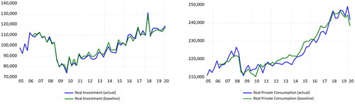
In this appendix, we show the performance of the model used in the paper by comparing the results from the simulations with actual data for the period under observation for the period 2005 to 2020. In the figures below, we compare the results from the simulation with the actual data for real GDP, real household consumption, total real investment and the level of employment.

Figure E1. Real GDP and employment, actual vs baseline model.

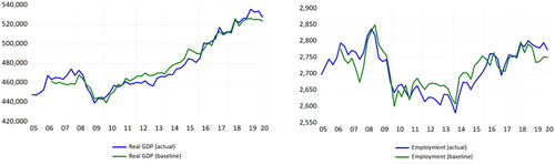
As can be seen in the left part of Figure E1, the model seems to be able to capture the dynamics of real economic activity quite accurately. While the model captures the evolution of the series in the period as a whole, it does seem to overshoot the economic activity in the period from 2011 to 2016. This overshooting can be explained by the fact that the model simulates both the level of investment (green line in the left panel of Figure E2) and consumption (green line in the right panel) too high compared to the actual data in 2011–2016 as seen in Figure E2.

Figure E2. Real investment (left) and real consumption (right).

Appendix F.

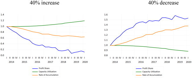
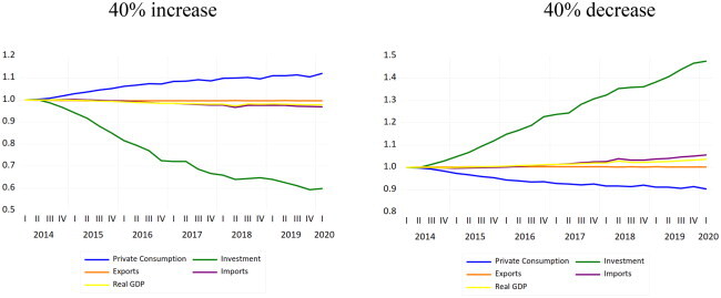
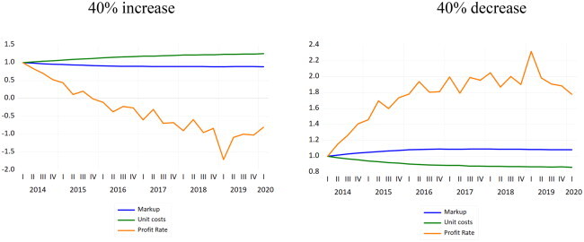
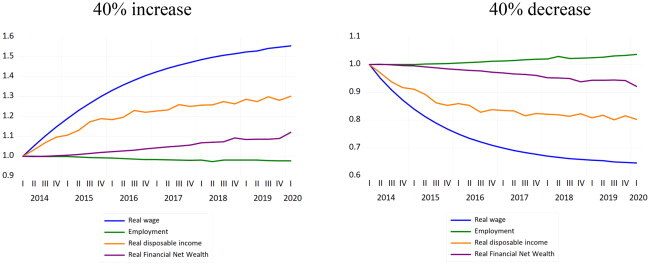
 Sensibility analysis

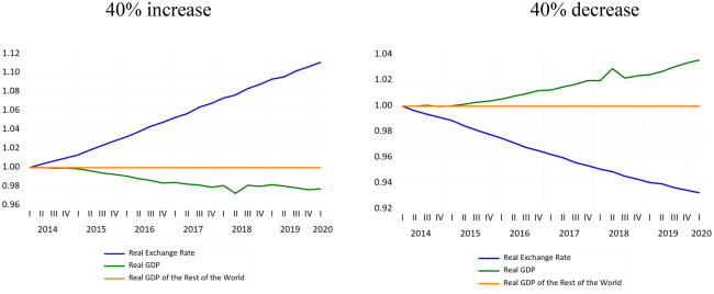
The simulation presented in the paper consisted of a 1% increase in trade union’s bargaining power. In order to generalize the conclusions drawn from the analysis it is necessary to check the robustness of the results, which is done by testing the same shock when the change in the respective parameter is larger and of the opposite sign. In other words, we want to make sure that our results are not dependent on the size of the shock. In the left-hand side, we show the case where there is a 40% increase in the bargaining power of unions, and in the right-hand side we show that the opposite results are found when there is a 40% decrease.

Impact of a change in the bargain power of workers

Impact of a change in the bargain power of workers

Impact of a change in the bargain power of workers

Impact of a change in the bargain power of workers

Impact of a change in the bargain power of workers

References

- Bengtsson, E., and E. Stockhammer. 2021. “Wages, Income Distribution and Economic Growth: Long-Run Perspectives in Scandinavia, 1900–2010.” Review of Political Economy 33 (4): 725–745. https://doi.org/10.1080/09538259.2020.1860307.
- Bhaduri, A., and S. Marglin. 1990. “Unemployment and the Real Wage: The Economic Basis for Contesting Political Ideologies.” Cambridge Journal of Economics 14 (4): 375–393. https://doi.org/10.1093/oxfordjournals.cje.a035141.
- Blecker, R. A. 1989. “International Competition, Income Distribution and Economic Growth.” Cambridge Journal of Economics 13 (3): 395–412.
- Blecker, R. A. 2016. “Wage-Led versus Profit-Led Demand Regimes: The Long and the Short of It.” Review of Keynesian Economics 4 (4): 373–390. https://doi.org/10.4337/roke.2016.04.02.
- Bowles, S., and R. Boyer. 1988. “Labor Discipline and Aggregate Demand: A Macroeconomic Model.” The American Economic Review 78 (2): 395–400.
- Byrialsen, M. R., H. Raza, and S. Valdecantos. 2022. QMDE: A quarterly empirical model for the Danish economy. A stock-flow consistent approach (No. 79). FMM Working Paper.
- Byrialsen, M. R., H. Raza, and S. Valdecantos. 2024. “Wage-Led or Profit-Led: Is It the Right Question to Examine the Relationship between Income Inequality and Economic Growth? Insights from an Empirical Stock-Flow Consistent Model for Denmark.” Cambridge Journal of Economics 48 (2): 303–328. [Forthcoming] https://doi.org/10.1093/cje/bead054.
- Charpe, M., S. Bridji, and P. McAdam. 2020. “Labor Share and Growth in the Long Run.” Macroeconomic Dynamics 24 (7): 1720–1757. https://doi.org/10.1017/S1365100518001025.
- Dodig, N., E. Hein, and D. Detzer. 2016. Financialisation and the Financial and Economic Crises: Theoretical Framework and Empirical Analysis for 15 Countries. Cheltenham: Edward Elgar Publishing.
- Dutt, A. K. 1984. “Stagnation, Income Distribution and Monopoly Power.” Cambridge Journal of Economics 8 (1): 25–40.
- Hein, E. 2014. Distribution and Growth after Keynes: A Post-Keynesian Guide. Cheltenham, UK: Edward Elgar Publishing.
- Hein, E., and L. Vogel. 2007. “Distribution and Growth Reconsidered: empirical Results for Six OECD Countries.” Cambridge Journal of Economics 32 (3): 479–511. https://doi.org/10.1093/cje/bem047.
- Kalecki, M. 1971. Selected Essays on the Dynamics of the Capitalist Economy, 1933–1970. Cambridge: Cambridge University Press.
- Marglin, S. A., and A. Bhaduri. 1991. “Profit Squeeze and Keynesian Theory.” In The Golden Age of Capitalism: reinterpreting the Postwar Experience, edited by Marglin, S. A. and Schor, J. B. New York: Oxford University Press.
- Obst, T., Ö. Onaran, and M. Nikolaidi. 2017. The effect of income distribution and fiscal policy on growth, investment, and budget balance: the case of Europe (No. 10). FMM Working Paper.
- Onaran, O., and T. Obst. 2016. “Wage-Led Growth in the EU15 Member-States: The Effects of Income Distribution on Growth, Investment, Trade Balance and Inflation.” Cambridge Journal of Economics 40 (6): 1517–1551. https://doi.org/10.1093/cje/bew009.
- Oyvat, C., O. Öztunalı, and C. Elgin. 2020. “Wage‐Led Versus Profit‐Led Demand: A Comprehensive Empirical Analysis.” Metroeconomica 71 (3): 458–486. https://doi.org/10.1111/meca.12284.
- Raza, H., T. Laurentjoye, M. R. Byrialsen, and S. Valdecantos. 2023. “Inflation and the Role of Macroeconomic Policies: A Model for the Case of Denmark.” Structural Change and Economic Dynamics 67: 32–43. https://doi.org/10.1016/j.strueco.2023.06.006.
- Rowthorn, R. E. 1981. Demand, Real Wages and Economic Growth. London: Thames Polytechnic.
- Santos, J. F. C., and R. A. Araujo. 2020. “Using Non-Linear Estimation Strategies to Test an Extended Version of the Goodwin Model on the US Economy.” Review of Keynesian Economics 8 (2): 268–286. https://doi.org/10.4337/roke.2020.02.07.
- Skott, P. 2017. “Weaknesses of ‘Wage-Led Growth.” Review of Keynesian Economics 5 (3): 336–359. https://doi.org/10.4337/roke.2017.03.03.
- Stockhammer, E., and R. Wildauer. 2016. “Debt-Driven Growth? Wealth, Distribution and Demand in OECD Countries.” Cambridge Journal of Economics 40 (6): 1609–1634. https://doi.org/10.1093/cje/bev070.
- Storm, S., and C. M. Naastepad. 2012. “Macroeconomics beyond the NAIRU.” In Macroeconomics beyond the NAIRU. Cambridge, MA: Harvard University Press.