Kindergarten allocation in Norway: An integer programming approach

Abstract

Kindergartens are vital to society in many countries, and in Norway, the municipalities are the local authorities that facilitate a coordinated admission process involving all their kindergartens. Allocating children to kindergartens is a very time-consuming task that is usually done manually. Therefore, we propose two integer programming (IP) models to support this task. Both models include the children’s prioritized kindergarten, prioritization of children with special needs, siblings already placed in a kindergarten and traveling times, while the second (extended) model also ensures gender and age balance in the kindergartens. To solve the largest instances found in Norway, we propose a heuristic variable reduction scheme. The models are solved with a commercial solver and have been tested on real data from Tønsberg municipality, as well as on larger instances reflecting the municipalities of Trondheim and Oslo. The model solutions are compared to the solutions from the allocation scheme used in Tønsberg and it is shown that the optimization models provide significantly better solutions. The models are being implemented into an existing kindergarten administration software and will be tested by a few selected municipalities. If this is successful, it will be rolled out to more than 50 municipalities currently using this software.

Keywords:

• Kindergarten allocation
• integer programming
• case study
• operations research

1. Introduction

Norwegian municipalities spend 46 billion NOK yearly to cover kindergarten operations, equivalent to 15% of their expenses (UDIR., 2017a). Kindergartens have significant societal importance, making it possible for the parents to work, and have direct impact on early child development. According to The Norwegian Kindergarten Act, all children have an equal right to education, regardless of where they live, their gender, social and cultural background or any special needs (Kunnskapsdepartementet, 2011). Consequently, more than 280,000 children in Norway had kindergarten placement in 2017, corresponding to 91% of all children aged between one and five years, and as many as 97% of the ones in the age group three to five years (SSB. , 2018). While education for children past the age of six is compulsory, enrollment in kindergarten is optional. A child is entitled to a place in a kindergarten from August if the child has turned one by the end of August the same year.

The Kindergarten Act also states that municipalities are the local authorities for kindergartens. They must ensure that kindergartens are operated in accordance with current rules, and facilitate a coordinated admission process involving all kindergartens within the municipality. This process must take into account the distinctive profiles of the kindergartens, in addition to the requests and needs of its users, such as siblings wanting to attend the same kindergarten. Additionally, by law, children with special requirements have to be given priority. Therefore, those responsible within the municipality must keep an overview of the capacity, and together with the boards from the kindergartens, treat the applications as well as prioritize and assign seats. In most cases, the kindergarten allocation is characterized by manual and time-consuming processes that can last for several months.

The Kindergarten Allocation Problem (KAP) consists of determining an optimal allocation of children to the kindergarten and is a special version of the general matching problem with preferences, which was surveyed by Biró (2017). The KAP is not a heavily studied problem within the operations research literature. However, it seems that the few papers largely agree on some important aspects to optimize. Both Veski, Biró, Põder, and Lauri (2017) and Kennes, Monte, and Tumennasan (2014) agree that outside of regulatory requirements, children with siblings already placed in a kindergarten should have priority. Veski et al. (2017) argue that distance from home to kindergarten also should be taken into account. Their paper discusses several representations of distance, such as distance zones. The distance zones in Veski et al. (2017) only represent kindergartens within walking distance, while the mathematical model presented in this paper divides kindergartens into three zones; walking distance, short driving distance, and outside of short driving distance. Kennes et al. (2014), which study the KAP in Denmark, propose a modified version of the deferred acceptance (DA) algorithm presented in Gale and Shapley (1962), while Veski et al. (2017) solve multiple versions of their problem with the original DA algorithm. This is where our work really distinguishes itself from previous research, as no previous studies use integer programming (IP) to solve the KAP.

The KAP has similarities also to other matching problems with preferences, see for example Church and Schoepfle (1993), Ehlers, Hafalir, Yenmez, and Yildirim (2014) and Sutcliffe, Board, and Cheshire (1984) for school assignment, and Roth (1984) and Kwanashie and Manlove (2014) for hospital/residents assignment.

The purpose of this paper is to propose two alternative IP models to solve the KAP and make the process more efficient, objective and fair, while still obeying all formal laws. The IP models have been used in a pilot project with Tønsberg municipality, with about 2200 children and 43 kindergartens, but also tested on larger instances to show the scalability of the models. Compared to the manual solution, which can take several months to produce, the IP models can be solved within minutes and provide significantly better solutions. The models can also be used to create a set of solutions that are equally good but exhibit different characteristics. One of the two models (denoted the extended model) is also able to take into account gender and age balance, which today’s manual process completely ignores.

The main contribution of this paper is a real case study where novel IP models provide valuable decision support and are shown to have a huge positive impact for society. This work has been done in collaboration with a Norwegian municipality and Visma. Visma is a provider of business software and services and has a cloud-based service named Visma Flyt Barnehage (VFB), used by more than 50 Norwegian municipalities to administer their kindergartens (Visma, 2018). In addition to being an administration tool to keep track of all children and kindergartens, the service also provides all the necessary data about the admission process to be able to go from a manual allocation to a digitalized solution for the allocation of children to kindergartens. By integrating the models into VFB, which is now being done, the allocation can be done without the need for manual work, as all the input data and updates are taken care of within the software.

The remainder of the paper is organized as follows. The KAP is formally described in Section 2, while the two models are presented in Section 3. The computational study is shown in Section 4, before we conclude in Section 5.

2. The kindergarten allocation problem

When parents apply for kindergarten placement on behalf of their children, they have to complete an application form. The application includes information such as gender, age, home address and siblings already placed in a kindergarten. Together with this information, the parents provide a prioritized list of the top three preferred kindergartens. In addition, the application describes which days the child require placement, e.g. every day except for Fridays. The kindergarten can then offer the available place on Fridays to another child. Therefore, the capacity requirement for kindergartens will restrict the total number of children placed in the kindergarten each weekday. However, a child can only be placed in one kindergarten, i.e. it cannot be placed in one kindergarten some days of the week and in another the remaining weekdays. The rules and regulations that Norwegian municipalities follow state that a full-time request should not be prioritized over a part-time request.

Kindergartens have certain requirements to fulfill when allocating the children, some that are strict, while others are soft (or objectives). First of all, kindergartens have a strict capacity on how many children they can accommodate. This number is based on the total floor and outdoor space, in addition to how many employees they have. Some kindergartens are exclusive to certain age groups. For instance, a few kindergartens only accept children between the age of zero and two years.

In addition to kindergarten specific requirements, regulatory requirements state that children with functional impairment get their priorities first as long as there is available capacity. Children who are the objects of an administrative decision of the Child Welfare Service Act also get priority. For the rest of this paper, these children are referred to as children with special requirements.

There are also some soft or guiding requirements when placing children in kindergartens. Even though it is not a requirement by law that siblings are placed in the same kindergarten, it is very much desired by the parents. Other soft requirements concern the driving distance between the children’s home and their assigned kindergarten, as well as both the age and gender distribution in each kindergarten.

The kindergarten allocation problem (KAP) can simply be defined as to determine the “optimal” allocation of children to kindergartens. However, a wide range of solutions can be found when optimizing the different objectives. For example, the number of children getting their first priority could be a good measurement of utility, but this would most likely result in many children not being allocated to any of their prioritized kindergartens. The problem can thus be described as one with multiple objectives, with different weights representing how important each objective is. These weights are subjective depending on what perspective one takes when solving the allocation. For this paper it is assumed that the following should be in the objective:

• Children placed in a prioritized kindergarten, where higher priority is better

• Children placed in the same kindergarten as their sibling

• Distance from each children’s home to the assigned kindergarten

3. Mathematical formulations

In this section we propose two integer programming (IP) models for the KAP. We start in Section 3.1 by presenting the notations and definitions used in both models, before presenting what we have denoted as the basic model in Section 3.2. An extended model, which also includes additional constraints and terms in the objective function to handle age and gender balance in the kindergartens, as well as the minimization of the maximum driving time for the parents, is presented in Section 3.3. To ease the solvability of the models, we propose a variable reduction scheme in Section 3.4.

3.1. Notation

This section introduces the sets, indices, parameters and variables used in the mathematical models.

3.1.1. Sets and indices

The set of children that have applied for kindergarten is denoted by $\mathcal{C},$ and the index c is used to reference elements in the set. The set of children is split up in different subsets, namely children with special requirements, children without special requirements, young children, and old children, denoted by ${\mathcal{C}}^S,{\mathcal{C}}^H,{\mathcal{C}}^Y$ and ${\mathcal{C}}^O,$ respectively, where $\mathcal{C}={\mathcal{C}}^S\cup {\mathcal{C}}^H$ and $\mathcal{C}={\mathcal{C}}^Y\cup {\mathcal{C}}^O.$ The set representing the available kindergartens is denoted $\mathcal{K}$ and referenced by the index k. We introduce two subsets of kindergartens, namely kindergartens only accepting young children (0 − 2 years) and kindergartens only accepting old children (3 − 5 years), denoted ${\mathcal{K}}^Y$ and ${\mathcal{K}}^O,$ respectively. We introduce a dummy kindergarten, denoted by the parameter $K^D,$ which is included in $\mathcal{K}.$ This means that children not being placed in a kindergarten are assigned to $K^D$ in the model.

Some children apply for a place in kindergarten only on specific weekdays. To handle this, the set of weekdays denoted by $\mathcal{D}$ is introduced and referenced by the index d.

3.2.2. Parameters

Kindergarten k has a given capacity of children for each day given by ${\overline{Q}}_{kd}.$ O_cd is a binary parameter, where 1 indicates that child c wants kindergarten placement on day d. Each child provides a prioritized list of three kindergartens when applying for a kindergarten seat. $P_{ck}^1,P_{ck}^2$ and $P_{ck}^3$ are either 0 or 1, where 1 indicates that child c ranks kindergarten k as first, second or third, respectively. The parameters $K_c^1,K_c^2,$ and $K_c^3$ are also introduced, which represent the kindergartens that are the first, second and third choice, respectively, of child c. In other words, $K_c^v=k$ if $P_{ck}^v=1,$ for v = 1, 2, 3. The binary parameter S_ck is 1 if child c has one or more siblings in kindergarten k, and 0 otherwise.

Traveling times are divided into three zones, where the binary parameter $T_{ck}^W$ is 1 if the traveling time between child c and kindergarten k is classified as walking distance. The same applies for short driving distance with $T_{ck}^D$ and for distances greater than short driving distance with $T_{ck}^F.$ Therefore, only one of these parameters are set to 1, while the two others are 0.

The mathematical models introduce seven weights, where W₁ is the penalty for a child that does not get a place in any kindergarten, while W₂ and W₃ are the penalties for children not getting their second and third priority, respectively. The weight parameter W₄ is the penalty for children not getting any of their priorities, while W₅ is the penalty for children not getting a seat in the same kindergarten as their siblings. Finally, W₆ and W₇ are penalties for children being placed in kindergartens outside of walking distance and driving distance, respectively.

3.2.3. Variables

The models introduce three types of binary variables. The solution to the problem is given by the x_ck variable, which is 1 if child c is placed in kindergarten k, and 0 otherwise. q_c is 1 if child c is placed in a different kindergarten than its sibling, and 0 if it does not have a sibling or it is placed in the same kindergarten as its sibling.

The next three variables ${\delta }_k^1,{\delta }_k^2,{\delta }_k^3$ are 1 if all children with special requirements that have kindergarten k as first, second, or third choice, respectively, are placed in kindergarten k or a kindergarten with higher priority on their list, else 0. Lastly, δ_k is 1 if and only if ${\delta }_k^1,{\delta }_k^2,{\delta }_k^3$ are all 1. Hence, this variable indicates if all children with special requirements with kindergarten k on their priority list are placed.

3.2. Basic model

3.2.1. Objective function

The objective function (1)(1) $$\begin{array}{c}\min z=\sum _{c\in \mathcal{C}}(W_1·x_{c{K}^D}+W_2·x_{c{K}_c^2}+W_3·x_{c{K}_c^3}+W_4·\sum _{k\in \mathcal{K}\setminus \{K_c^1,K_c^2,K_c^3,K^D\}}{x}_{ck}\hfill \\ +W_5·q_c+W_6·\sum _{k\in \mathcal{K}\setminus \{K_c^1,K_c^2,K_c^3,K^D\}}{T}_{ck}^D·x_{ck}+W_7·\sum _{k\in \mathcal{K}\setminus \{K_c^1,K_c^2,K_c^3,K^D\}}{T}_{ck}^F·x_{ck})\hfill \end{array}$$(1) consists of seven terms with associated weights. The first term represents the cost of not placing children in any kindergarten. The next three terms represent the cost of children not getting a kindergarten that is their first, second, or third priority, respectively. The fifth term penalizes siblings not being placed in the same kindergarten. Finally, the last two terms penalize children who do not get any of their priorities and are placed in kindergartens outside of walking distance and short driving distance, respectively. (1) $$\begin{array}{c}\min z=\sum _{c\in \mathcal{C}}(W_1·x_{c{K}^D}+W_2·x_{c{K}_c^2}+W_3·x_{c{K}_c^3}+W_4·\sum _{k\in \mathcal{K}\setminus \{K_c^1,K_c^2,K_c^3,K^D\}}{x}_{ck}\hfill \\ +W_5·q_c+W_6·\sum _{k\in \mathcal{K}\setminus \{K_c^1,K_c^2,K_c^3,K^D\}}{T}_{ck}^D·x_{ck}+W_7·\sum _{k\in \mathcal{K}\setminus \{K_c^1,K_c^2,K_c^3,K^D\}}{T}_{ck}^F·x_{ck})\hfill \end{array}$$(1)

The objective function (1)(1) $$\begin{array}{c}\min z=\sum _{c\in \mathcal{C}}(W_1·x_{c{K}^D}+W_2·x_{c{K}_c^2}+W_3·x_{c{K}_c^3}+W_4·\sum _{k\in \mathcal{K}\setminus \{K_c^1,K_c^2,K_c^3,K^D\}}{x}_{ck}\hfill \\ +W_5·q_c+W_6·\sum _{k\in \mathcal{K}\setminus \{K_c^1,K_c^2,K_c^3,K^D\}}{T}_{ck}^D·x_{ck}+W_7·\sum _{k\in \mathcal{K}\setminus \{K_c^1,K_c^2,K_c^3,K^D\}}{T}_{ck}^F·x_{ck})\hfill \end{array}$$(1) is to be minimized subject to the following sets of constraints.

3.2.2. Allocation and capacity

Constraints (2)(2) $$\sum _{k\in \mathcal{K}}{x}_{ck}=1c\in \mathcal{C}$$(2) ensure that every child is placed in exactly one kindergarten or not placed at all. As mentioned earlier, the children that are not placed are assigned to a dummy kindergarten with unlimited capacity. Constraints (3)(3) $$\sum _{c\in \mathcal{C}}{O}_{cd}·x_{ck}-{\overline{Q}}_{kd}\le 0k\in \mathcal{K}\setminus \left\{K^D\right\},d\in \mathcal{D}$$(3) make sure that the capacity for each kindergarten for each day is not exceeded. (2) $$\sum _{k\in \mathcal{K}}{x}_{ck}=1c\in \mathcal{C}$$(2) (3) $$\sum _{c\in \mathcal{C}}{O}_{cd}·x_{ck}-{\overline{Q}}_{kd}\le 0k\in \mathcal{K}\setminus \left\{K^D\right\},d\in \mathcal{D}$$(3)

3.2.3. Prioritizing siblings and children with special requirements

Constraints (4)(9) $$x_{ck}-{\delta }_k\le 0c\in {\mathcal{C}}^H,k\in \mathcal{K}$$(9) force q_c to take the value of 1 if child c is placed in a different kindergarten than its sibling. Constraints (5)(5) $$\sum _{c\in {\mathcal{C}}^S}(P_{ck}^1·{\delta }_k^1-x_{ck})\le 0\hspace{0.5em}k\in \mathcal{K}\setminus \left\{K^D\right\}$$(5) –(9)(9) $$x_{ck}-{\delta }_k\le 0c\in {\mathcal{C}}^H,k\in \mathcal{K}$$(9) enforce the placement of children with special requirements before placing other children. The first type of constraint (5)(5) $$\sum _{c\in {\mathcal{C}}^S}(P_{ck}^1·{\delta }_k^1-x_{ck})\le 0\hspace{0.5em}k\in \mathcal{K}\setminus \left\{K^D\right\}$$(5) enforce that ${\delta }_k^1$ can only be 1 if all children with special requirements that have put kindergarten k as their first priority are placed in kindergarten k. Likewise, constraints (6)(6) $$\sum _{c\in {\mathcal{C}}^S}(P_{ck}^2·({\delta }_k^2-\sum _{k^{*}\in \mathcal{K}\setminus \left\{K^D\right\}}(P_{c{k}^{*}}^1·x_{c{k}^{*}})-x_{ck}))\le 0k\in \mathcal{K}\setminus \left\{K^D\right\}$$(6) make sure that ${\delta }_k^2$ can only be 1 if all children with special requirements that have put kindergarten k as their second priority are placed in kindergarten k or their first priority. Constraints (7)(7) $$\sum _{c\in {\mathcal{C}}^S}(P_{ck}^3·({\delta }_k^3-\sum _{k^{*}\in \mathcal{K}\setminus \left\{K^D\right\}}((P_{c{k}^{*}}^1+P_{c{k}^{*}}^2)·x_{c{k}^{*}})-x_{ck}))\le 0k\in \mathcal{K}\setminus \left\{K^D\right\}$$(7) do exactly the same for third priorities. These δ-variables (${\delta }_k^1,{\delta }_k^2,{\delta }_k^3$) are then combined into δ_k in constraints (8)(8) $$3·{\delta }_k-{\delta }_k^1-{\delta }_k^2-{\delta }_k^3\mathrm{}\le 0\mathrm{\hspace{1em}}k\in \mathcal{K}$$(8) so that δ_k can only be 1 if all three aforementioned variables are 1. Constraints (9)(9) $$x_{ck}-{\delta }_k\le 0c\in {\mathcal{C}}^H,k\in \mathcal{K}$$(9) then enforce that the children without special requirements can only be placed in kindergarten k if all children with special requirements that have kindergarten k as a priority are placed first. (4) $$\sum _{k\in \mathcal{K}\setminus \left\{K^D\right\}}(S_{ck}·(1-x_{ck}))-q_c\le 0c\in \mathcal{C}$$(4) (5) $$\sum _{c\in {\mathcal{C}}^S}(P_{ck}^1·{\delta }_k^1-x_{ck})\le 0\hspace{0.5em}k\in \mathcal{K}\setminus \left\{K^D\right\}$$(5) (6) $$\sum _{c\in {\mathcal{C}}^S}(P_{ck}^2·({\delta }_k^2-\sum _{k^{*}\in \mathcal{K}\setminus \left\{K^D\right\}}(P_{c{k}^{*}}^1·x_{c{k}^{*}})-x_{ck}))\le 0k\in \mathcal{K}\setminus \left\{K^D\right\}$$(6) (7) $$\sum _{c\in {\mathcal{C}}^S}(P_{ck}^3·({\delta }_k^3-\sum _{k^{*}\in \mathcal{K}\setminus \left\{K^D\right\}}((P_{c{k}^{*}}^1+P_{c{k}^{*}}^2)·x_{c{k}^{*}})-x_{ck}))\le 0k\in \mathcal{K}\setminus \left\{K^D\right\}$$(7) (8) $$3·{\delta }_k-{\delta }_k^1-{\delta }_k^2-{\delta }_k^3\mathrm{}\le 0\mathrm{\hspace{1em}}k\in \mathcal{K}$$(8) (9) $$x_{ck}-{\delta }_k\le 0c\in {\mathcal{C}}^H,k\in \mathcal{K}$$(9)

3.2.4. Variable definitions

The binary definitions of the variables are given by constraints (10) – (12). To reduce the number of variables, we do not define x_ck for the infeasible combinations due to children’s age and the kindergarten’s age profile. (10) $$x_{ck}\in \{0,1\}c\in \mathcal{C},k\in \mathcal{K}$$(10) (11) $$q_c\in \{0,1\}c\in \mathcal{C}$$(11) (12) $${\delta }_k,{\delta }_k^1,{\delta }_k^2,{\delta }_k^3\in \{0,1\}k\in \mathcal{K}$$(12)

3.3. Extended model

This section presents the extended model that also takes into account gender and age balance, as well as a more detailed way to reduce traveling time for the parents.

3.3.1. Gender balance

Even though it is usually not used as a criterion in the kindergarten allocation, an even gender balance in the kindergartens is desired. Gender balance could be added to the model by adding (soft) gender limits for each kindergarten. This extension would add constraints by penalizing allocations that have kindergartens with a gender imbalance in the objective function. To do this, we introduce the parameters G_c, which is 1 if child c is male, and 0 if female, while ${\underset{¯}{G}}_k$ and ${\overline{G}}_k$ are the lower and upper target limits, respectively, on the number of children of the same gender in kindergarten k. E.g. a kindergarten with a capacity of ten children could have an upper target limit of seven and a lower target limit of three for both genders. Furthermore, we impose a cost to the number of kindergartens that violates these target limits. The new binary variable g_k, penalized in the objective function, is added to allow the gender limits to be violated if g_k is set to 1.

We can then add the following new constraints (13)(13) $$\sum _{c\in \mathcal{C}}{G}_c·x_{ck}\le {\overline{G}}_k+M·g_{k}k\in \mathcal{K},d\in \mathcal{D}$$(13) and (14)(14) $$\sum _{c\in \mathcal{C}}{G}_c·x_{ck}\ge {\underset{¯}{G}}_k·(1-g_k)k\in \mathcal{K},d\in \mathcal{D}$$(14) , while the objective function will get an additional term (shown later in this section). The M in constraints (13)(13) $$\sum _{c\in \mathcal{C}}{G}_c·x_{ck}\le {\overline{G}}_k+M·g_{k}k\in \mathcal{K},d\in \mathcal{D}$$(13) is calculated as $({\overline{Q}}_{kd}-{\overline{G}}_{kd}).$ (13) $$\sum _{c\in \mathcal{C}}{G}_c·x_{ck}\le {\overline{G}}_k+M·g_{k}k\in \mathcal{K},d\in \mathcal{D}$$(13) (14) $$\sum _{c\in \mathcal{C}}{G}_c·x_{ck}\ge {\underset{¯}{G}}_k·(1-g_k)k\in \mathcal{K},d\in \mathcal{D}$$(14)

3.3.2. Age balance

An even age distribution is also desired by many kindergartens. As for the gender balance, we model this with soft constraints and penalize the number of kindergartens breaking the constraints in the objective function. A new variable a_k, which is penalized with an additional term in the objective function, is added to allow the age limits to be violated if it is set to 1. We also define the binary parameter Y_ca to be 1 if child c is of age a, and 0 otherwise, while ${\underset{¯}{L}}_{ka}$ and ${\overline{L}}_{ka}$ are respectively the lower and upper limits of children of age a that can be placed in kindergarten k. Furthermore, we add the following new constraints (15)(15) $$\sum _{c\in \mathcal{C}}{O}_{cd}·Y_{ca}·x_{ck}\le {\overline{L}}_{ka}+M·a_{k}k\in \mathcal{K},d\in \mathcal{D},a\in \mathcal{A}$$(15) and (16)(16) $$\sum _{c\in \mathcal{C}}{O}_{cd}·Y_{ca}·x_{ck}\ge {\underset{¯}{L}}_{ka}·(1-a_k)k\in \mathcal{K},d\in \mathcal{D},a\in \mathcal{A}$$(16) . The big-M is chosen as small as possible to obtain a tight formulation, and calculated as $({\overline{Q}}_k-{\overline{L}}_{ka}).$ (15) $$\sum _{c\in \mathcal{C}}{O}_{cd}·Y_{ca}·x_{ck}\le {\overline{L}}_{ka}+M·a_{k}k\in \mathcal{K},d\in \mathcal{D},a\in \mathcal{A}$$(15) (16) $$\sum _{c\in \mathcal{C}}{O}_{cd}·Y_{ca}·x_{ck}\ge {\underset{¯}{L}}_{ka}·(1-a_k)k\in \mathcal{K},d\in \mathcal{D},a\in \mathcal{A}$$(16)

3.3.3. Traveling time

Even though traveling time is to some extent included in the basic model, we also add in the extended model a new penalty term in the objective function for the longest traveling time any child experiences. This is to ensure that nobody gets a kindergarten very far away, which can be considered as both inconvenient and unfair. To achieve this, we introduce a traveling time parameter T_ck that represents the traveling time from child c to kindergarten k and a new variable t^max, as well as the following additional constraints (17)(17) $$\sum _{k\in \mathcal{K}\setminus \{K_c^1,K_c^2,K_c^3,K^D\}}{T}_{ck}·x_{ck}\le t^{\mathit{max}}c\in \mathcal{C}$$(17) . (17) $$\sum _{k\in \mathcal{K}\setminus \{K_c^1,K_c^2,K_c^3,K^D\}}{T}_{ck}·x_{ck}\le t^{\mathit{max}}c\in \mathcal{C}$$(17)

3.3.4. New objective function

The extended model consists of the constraints (2)(2) $$\sum _{k\in \mathcal{K}}{x}_{ck}=1c\in \mathcal{C}$$(2) –(15)(15) $$\sum _{c\in \mathcal{C}}{O}_{cd}·Y_{ca}·x_{ck}\le {\overline{L}}_{ka}+M·a_{k}k\in \mathcal{K},d\in \mathcal{D},a\in \mathcal{A}$$(15) from the basic model, plus the new constraints (13)(13) $$\sum _{c\in \mathcal{C}}{G}_c·x_{ck}\le {\overline{G}}_k+M·g_{k}k\in \mathcal{K},d\in \mathcal{D}$$(13) –(17)(17) $$\sum _{k\in \mathcal{K}\setminus \{K_c^1,K_c^2,K_c^3,K^D\}}{T}_{ck}·x_{ck}\le t^{\mathit{max}}c\in \mathcal{C}$$(17) , while the extended objective function (18)(18) $$\begin{array}{c}\min z=\sum _{c\in \mathcal{C}}(W_1·x_{c{K}^D}+W_2·x_{c{K}_c^2}+W_3·x_{c{K}_c^3}+W_4·\sum _{k\in \mathcal{K}\setminus \{K_c^1,K_c^2,K_c^3,K^D\}}{x}_{ck}\\ +W_5·q_c+W_6·\sum _{k\in \mathcal{K}\setminus \{K_c^1,K_c^2,K_c^3,K^D\}}{T}_{ck}^D·x_{ck}+W_7·\sum _{k\in \mathcal{K}\setminus \{K_c^1,K_c^2,K_c^3,K^D\}}{T}_{ck}^F·x_{ck})\\ +W_8·\sum _{k\in \mathcal{K}\setminus \left\{K^D\right\}}{g}_k+W_9·\sum _{k\in \mathcal{K}\setminus \left\{K^D\right\}}{a}_k+W_{10}·t^{\mathit{max}}\end{array}$$(18) now includes three additional terms with the weighting factors W₈, W₉ and W₁₀ for the gender and age imbalance and the traveling time, respectively: (18) $$\begin{array}{c}\min z=\sum _{c\in \mathcal{C}}(W_1·x_{c{K}^D}+W_2·x_{c{K}_c^2}+W_3·x_{c{K}_c^3}+W_4·\sum _{k\in \mathcal{K}\setminus \{K_c^1,K_c^2,K_c^3,K^D\}}{x}_{ck}\\ +W_5·q_c+W_6·\sum _{k\in \mathcal{K}\setminus \{K_c^1,K_c^2,K_c^3,K^D\}}{T}_{ck}^D·x_{ck}+W_7·\sum _{k\in \mathcal{K}\setminus \{K_c^1,K_c^2,K_c^3,K^D\}}{T}_{ck}^F·x_{ck})\\ +W_8·\sum _{k\in \mathcal{K}\setminus \left\{K^D\right\}}{g}_k+W_9·\sum _{k\in \mathcal{K}\setminus \left\{K^D\right\}}{a}_k+W_{10}·t^{\mathit{max}}\end{array}$$(18)

3.4. Variable reduction

In both models presented above, a binary variable x_ck is created for each possible matching between a child and a kindergarten. This causes the number of variables to grow quadratically with the instance size. However, each child only prioritizes three kindergartens and those who do not get any of their priorities should be placed in nearby kindergartens. Hence, all variables representing the placement of a child in a kindergarten far away will usually become 0. This is exploited by not generating the x_ck-variables where the traveling time between child c and kindergarten k is more than a predefined cut-off distance D, which will reduce the size of the model. This is a heuristic, but with a reasonable choice of D, the solutions may still be (near-)optimal.

4. Computational study

This section presents the results from testing the IP models on test instances for three Norwegian cities/municipalities. All testing is done using the IP solver Xpress on a desktop computer with 3.4 GHz Intel i7 processor and 32GB of RAM. We set a limit on the maximum running time to three hours.

4.1. Test instances and setting of penalty weights

This section describes the test instances, summarized in Table 1. These instances represent three different Norwegian municipalities: Tønsberg, Trondheim, and Oslo. The smallest instance size, Tønsberg, includes 2170 children and 43 kindergartens. Travel times and the weekdays a child requires kindergarten placement are obtained from Visma. The rest of the necessary data is generated according to the test instance framework described below. The two last instance sizes, named Trondheim and Oslo, consist of 10343 children and 182 kindergartens, and 36230 children and 605 kindergartens, respectively (UDIR, 2017b). The only real data for these instances are the number of children and kindergartens, and the capacities of the kindergartens. The rest is generated as described below. For each instance size, ten different instances are created, resulting in a total of 30 test instances. For the Trondheim and Oslo instances, the traveling times are generated based on the traveling time distribution from Tønsberg.

Table 1. Overview of test instance sizes.

Instance sizes	# Children	# Kindergartens
Tønsberg	2170	43
Trondheim	10343	182
Oslo	36230	605

The traveling times are divided into three zones, indicated by the binary parameters $T_{ck}^W,T_{ck}^D$ and $T_{ck}^F$ for each child c and kindergarten k. If the driving time is below 300 s, it is classified as “walking zone”, i.e. $T_{ck}^W=1.$ If the driving time is between 300 and 600 s, it is classified as “driving zone”, i.e. $T_{ck}^D=1.$ In cases where the driving time is greater than 600 s, the given kindergarten are classified as being “outside of driving zone”, i.e. $T_{ck}^F=1.$

Among the children attending kindergartens in Norway, 3.1% have special requirements (Bufdir, 2018). It is assumed that this number is representative for the three municipalities. Hence, 3.1% of the children (randomly chosen) are included in the set ${\mathcal{C}}^S$ defined in Section 3. We assume an 80% probability that children will choose the three closest kindergartens, with the closest as a first priority, and so on. For the remaining 20%, we assume they choose three random kindergartens. In both cases, the age profile requirement of each kindergarten has to be satisfied.

Among the children attending kindergartens in Tønsberg, 20% have siblings in kindergartens. It is assumed that this number is representative also for Trondheim and Oslo municipality. It is also assumed that if a child has a sibling in a kindergarten, it will put this kindergarten as its first priority. Hence, children are generated with a 20% chance of having a sibling in their highest prioritized kindergarten.

It is obvious that different penalty weights, W₁ – W₁₀, may give alternative solutions. The weights are therefore carefully chosen after preliminary testing and close discussions with Tønsberg municipality to represent the how they prioritize. W₁ is the largest weight for both models since placing as many children as possible in kindergartens is most important. The second most important aspect is to place children in the same kindergarten as their siblings. Hence, W₅ is the second largest weight. The kindergarten priority weights, W₂ – W₄, are ordered by the priority, such that $W_4>W_3>W_2.$ The traveling time weights, W₆ and W₈, are also ordered, where increasing traveling time is penalized with a higher weight, i.e. $W_7>W_6.$ For the extended model, the last three weights, W₈ – W₁₀, represent the costs of a kindergarten breaking the gender limits, age limits, and the longest traveling time for the children placed in non-prioritized kindergartens. These weights are also set after preliminary testing. For practical reasons, all weight parameters are stipulated so that the sum of all equals one. We have based on this reached the following setting of the weights: $$\text{Basic}\mathrm{}\text{model}\mathrm{}(W_1–W_7):\mathrm{}0.31,\mathrm{}0.05,\mathrm{}0.10,\mathrm{}0.15,\mathrm{}0.29,\mathrm{}0.03,\mathrm{}0.07$$ $$\text{Extended}\mathrm{}\text{model}\mathrm{}\left(W_1–W_{10}\right):\mathrm{}0.27,\mathrm{}0.03,\mathrm{}0.06,\mathrm{}0.09,\mathrm{}0.26,\mathrm{}0.02,\mathrm{}0.04,\mathrm{}0.11,\mathrm{}0.10,\mathrm{}0.01$$

4.2. Computational results

In this section, the performance of the basic and extended models is studied. The models are run on all test instance sizes introduced in Table 1, with ten instances of each test size. Average results for each instance size are summarized in Table 2 and include computation time until optimality (if reached before the maximum running time), optimality gap after one hour, and optimality gap after finished execution. The optimality gap is defined as the percentage difference between the current objective value and the best bound found by Xpress. The Oslo instances were run with the heuristic variable reduction scheme presented in Section 3.4.

Table 2. Computational time, optimality gap after one hour, optimality gap after three hours, LP objective value and IP objective value for the basic and extended model. The Oslo instances were run with variable reduction.

Model	Instance size		Comp. time (s)	Gap 1 h %	Gap %	LP	IP
		Min	10.7	0.0	0.0	59.78	60.18
	Tønsberg	Max	13.6	0.0	0.0	65.02	65.79
		Avg	12.4	0.0	0.0	61.97	62.46
		Min	778.4	0.0	0.0	143.14	143.42
Basic	Trondheim	Max	802.0	0.0	0.0	154.96	155.94
		Avg	786.6	0.0	0.0	148.27	148.60
		Min	1060.6	0.0	0.0	745.85	754.57
	Oslo	Max	1358.4	0.0	0.0	757.46	767.20
		Avg	1146.2	0.0	0.0	750.36	759.55
		Min	363.4	0.0	0.0	38.97	42.82
	Tønsberg	Max	>10800	3.40	1.75	42.96	47.85
		Avg	8916.7	1.89	0.72	40.73	44.69
		Min	>10800	1.43	1.03	89.08	95.37
Extended	Trondheim	Max	>10800	1.98	1.97	96.86	102.87
		Avg	>10800	1.63	1.47	92.36	98.14
		Min	>10800	0.24	0.13	458.32	480.36
	Oslo	Max	>10800	0.35	0.22	466.71	490.15
		Avg	>10800	0.28	0.17	461.46	483.80

For the basic model, the solver finds the optimal solution to all Tønsberg and Trondheim instances in approximately 12 s and 13 min, respectively. An interesting observation is that there are only small differences between the LP and IP objective values. The basic model gives, to a large extent, naturally binary solution variables, which can explain the short running times. Despite this, the solver runs out of memory before it can solve the Oslo instances, so the results for these instances in Table 2 are with variable reduction (explained in more detail further below).

The performance of the extended model is very different compared to the basic model. First, it takes significantly longer time to solve. The Tønsberg instances were solved to optimality in 12.4 s on average for the basic model, compared to 8916.7 s with an average gap of 0.72% for the extended model. None of the Trondheim instances were solved to optimality within three hours. Second, the variance of the computational times between instances of the same size is much higher for the extended model. One instance was solved to optimality in about five minutes, while others still were not solved after three hours. Third, the extended model does not provide naturally binary solution variables in the same manner as the basic model and have much larger differences between the LP and IP objective values, which can explain why the extended model takes significantly longer time solve.

After not being able to run the Oslo instances due to insufficient memory, variable reduction was applied as a heuristic to make the instances solvable. As described in Section 3.4, one would most likely not need all the x_ck-variables as the kindergartens far away from a child will rarely be used by that child in an optimal solution. To find an appropriate cut-off distance D (seconds), the model was run iteratively with increasing values for D to see when the objective value converged towards the optimal objective value. This was first done for the basic model on one chosen instance from both Tønsberg and Trondheim, and then for the extended model on the same instances. The models were only run for a maximum of 1800 s, as this provides solutions that are good enough to verify that the cut-off distance is appropriate for variable reduction. The results from this are shown in Figures 1–4.

Figure 1. The objective value vs. the run time of the basic model on one instance, with increasing cut-off distance for Tønsberg.

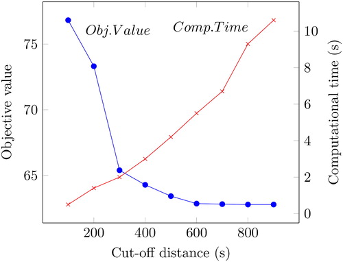
Figure 2. The objective value vs. the run time of the basic model on one instance, with increasing cut-off distance for Trondheim.

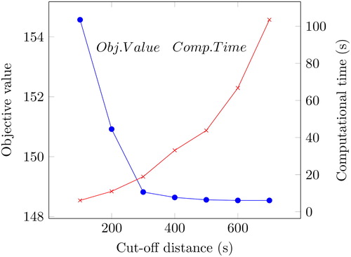
Figure 3. The objective value vs. the run time of the extended model on one instance, with increasing cut-off distance for Tønsberg.

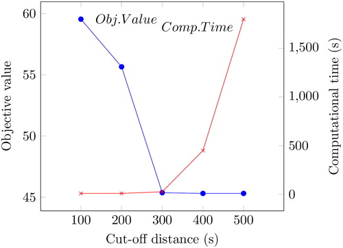
Figure 4. The objective value vs. the run time of the extended model on one instance, with increasing cut-off distance for Trondheim.

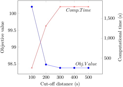
The tests show that, for all practical purposes, the results with variable reduction are as good as without. The solutions are even better for the extended model because it was not solved to optimality and had significant optimality gaps without variable reduction. From the plots, it is not obvious what cut-off distance to choose. The extended model can have a lower cut-off than the basic model, probably because the extended model penalizes solutions that give a large value for the maximum distance of a child not being placed in one of its prioritized kindergartens. Thus, the optimal solutions for the extended model have shorter distances for each child/kindergarten-pair in general. Another interesting fact is that it seems like one can accept shorter cut-off distances for Trondheim than for Tønsberg, even though the distances in Trondheim are 1.4 times longer on average than for Tønsberg. This can be explained by a higher kindergarten density in a larger city like Trondheim, making it easier to find one that is close.

The cut-off distances for Oslo were set to 700 and 400 s for the basic and extended model, respectively. These values correspond to the mean of the cut-off distances that gave optimal solutions. This is a conservative choice as it can be expected that one can have an even shorter cut-off distance for Oslo than on the Trondheim instances, following the argument in the previous paragraph.

With variable reduction, we were able to solve the Oslo instances to optimality within 20 min for the basic model, while the extended model reached an average optimality gap of 0.17% after 3 h, see Table 2. This is the same trend as for the two smaller instances. The models seem to scale well with variable reduction. Oslo is the biggest city in Norway, and the model reassigned all the children within a reasonable amount of time. In reality, the set of children would be smaller as only new applicants have to be assigned a kindergarten. The models therefore seem well suited for solving the KAP in all municipalities in Norway.

4.3. Comparison of solutions from the basic and extended models

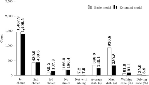
Figure 5 presents the aggregated results for the basic and extended model runs on the ten Tønsberg instances. There are a few important distinctions between the two. They place almost the same amount of children in a prioritized kindergarten, but the basic model places them in higher priorities. Distance is the aspect where there is the largest difference between the solutions from the two models. The average traveling time for a child is about 30% lower for the extended model and the difference is even larger for the maximum distance. This will also contribute to reduce driving, and hence reduced congestion and environmental emissions, which are very important aspects in the development of cities. Evidently, there is a trade-off between placing more children in higher priorities and traveling time for children getting a non-prioritized kindergarten.

Figure 5. The average solution of the basic model compared to the average solution of the extended model run on the ten Tønsberg instances.

We cannot claim that one model works better than the other, as this depends on how the different municipalities value the different objectives. Note also, as discussed in Section 4.1, that the solutions will depend on the weights of the penalty parameters in the objective function, and different solutions could be obtained by changing the weights.

4.4. Comparison with real planning solutions

The allocation of children to kindergartens in the municipalities is today done according to statutes that are decided by local politicians. In Tønsberg, the allocation is done greedily by giving each child a ranking and placing the highest ranked children first in their highest prioritized kindergarten that has available capacity. If all three prioritized kindergartens are full, the child is placed in the closest non-prioritized kindergarten with available capacity. There are four levels of rankings in Tønsberg (where the first two correspond to “special requirements” in our model):

1. Children with impaired functioning and children who are the objects of an administrative decision of the Child Welfare Service Act

2. Children from families who suffer from severe stress such as illness or disability

3. Children who have siblings already placed in a kindergarten

4. Remaining children sorted by age

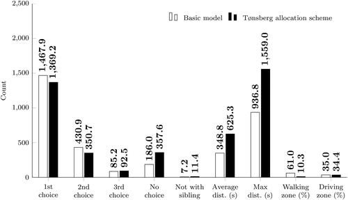
By comparing the solutions from the basic model with the solutions from the Tønsberg allocation scheme on the ten different Tønsberg instances, as illustrated in Figure 6, it is clear that the model outperforms today’s allocation scheme. More children get a prioritized kindergarten and they also get higher priorities, more children are placed in the same kindergarten as their siblings, and the children who are placed in non-prioritized kindergartens are placed in closer ones.

Figure 6. The average solution of the basic model compared to Tønsberg municipality’s greedy allocation scheme run on the ten Tønsberg instances.

5. Conclusions

This paper presented two new integer programming (IP) models to the Kindergarten Allocation Problem (KAP) and applied these to a real case for a Norwegian municipality. The objective of the IP models is to minimize the sum of penalties for not giving children their prioritized kindergartens, placing children in a different kindergarten than their sibling, and the distance a child has to travel if it does not get one of its prioritized kindergartens. The second extended model also includes terms to ensure a good gender and age balance in the kindergartens and to reduce the maximum driving distance for any child. To solve the largest instances found in Norway, we have also proposed a heuristic variable reduction scheme.

The IP models outperform the allocation scheme used by Tønsberg municipality on all objectives. Today, municipalities have to follow their statutes for allocating children to kindergartens, but this study shows why and how these statutes should be changed to obtain better solutions. The model is also tested on larger instances, and by performing variable reduction, the model can produce good solutions for any municipality in Norway in a reasonable time.

For the society, the results from the models could provide a better national standard for how to assign children to kindergartens. More children would get their preferred choices and driving distances can be reduced for the parents, with reduced congestion and emissions in cities as a positive side-effect. The promising results motivated Visma to implement the model into their existing software solution, Visma Flyt Barnehage (VFB), so as to utilize the data from this software to accommodate for a holistic kindergarten application and admission process. This will be tested further by a few selected municipalities on the 2020 kindergarten admissions, and if successful, it will be rolled out to the more than 50 municipalities currently using VFB.

Finally, even though this is a Norwegian case study, we believe the models and results presented in this paper can be adapted to KAPs also in other countries.

Disclosure statement

No potential conflict of interest was reported by the author(s).

References

- Biró, P. (2017). Applications of matching models under preferences. Trends in Computational Social Choice, 1, 345–373.
- Bufdir (2018). Kindergarten. https://www.bufdir.no/Statistikk_og_analyse/Nedsatt_funksjonsevne/Oppvekst_og_utdanning/Barnehage/?fbclid=IwAR2II4a__d6yt5ORi4arWY1T2WFN78yw4IntTVsHJSQU_5qXtr8e5mgK_bg
- Church, R. L., & Schoepfle, O. B. (1993). The choice alternative to school assignment. Environment and Planning B: Planning and Design, 20(4), 447–457. doi:10.1068/b200447
- Ehlers, L., Hafalir, I. E., Yenmez, M. B., & Yildirim, M. A. (2014). School choice with controlled choice constraints: Hard bounds versus soft bounds. Journal of Economic Theory, 153, 648–683. doi:10.1016/j.jet.2014.03.004
- Gale, D., & Shapley, L. S. (1962). College admissions and the stability of marriage. The American Mathematical Monthly, 69 (1), 9–15. doi:10.2307/2312726
- Kennes, J., Monte, D., & Tumennasan, N. (2014). The day care assignment: A dynamic matching problem. American Economic Journal: Microeconomics, 6, 362–406. doi:10.1257/mic.6.4.362
- Kunnskapsdepartementet. (2011). Act no. 64 of June 2005 relating to Kindergartens (the Kindergarten Act). https://www.regjeringen.no/globalassets/upload/kd/vedlegg/barnehager/engelsk/act_no_64_of_june_2005_web.pdf.
- Kwanashie, A., & Manlove, D. F. (2014). An integer programming approach to the hospitals/residents problem with ties. In Operations Research Proceedings 2013: Selected Papers of the International Conference on Operations Research, OR2013. Series: Operations Research Proceedings (pp. 263–269). Springer International Publishing. ISBN 9783319070001.
- Roth, A. E. (1984). The evolution of the labor market for medical interns and residents: A case study in game theory. Journal of Political Economy, 92 (6), 991–1016. doi:10.1086/261272
- SSB. (2018). Kindergartens. https://www.ssb.no/en/utdanning/statistikker/barnehager/.
- Sutcliffe, C., Board, J., & Cheshire, P. (1984). Goal programming and allocating children to secondary schools in reading. The Journal of the Operational Research Society, 35 (8), 719–730. doi:10.2307/2581978
- UDIR. (2017a). 4.2 Costs for kindergartens. http://utdanningsspeilet.udir.no/2017/innhold/del-4/4-2-kostnader-til-barnehage/
- UDIR. (2017b). Number of kindergartens. https://www.udir.no/tall-og-forskning/statistikk/statistikk-barnehage/antall-barnehager/
- Veski, A., Biró, P., Põder, K., & Lauri, T. (2017). Efficiency and fair access in kindergarten allocation policy design. Journal of Mechanism and Institution Design, 2(1), 57–104. doi:10.22574/jmid.2017.12.003
- Visma. (2018). Visma “Flyt Barnehage”. https://www.visma.no/oppvekst/barnehagesystem/