A hybrid model based on bidirectional long short-term memory neural network and Catboost for short-term electricity spot price forecasting

Abstract

Electricity price forecasting plays a crucial role in a liberalised electricity market. Generally speaking, long-term electricity price is widely utilised for investment profitability analysis, grid or transmission expansion planning, while medium-term forecasting is important to markets that involve medium-term contracts. Typical applications of medium-term forecasting are risk management, balance sheet calculation, derivative pricing, and bilateral contracting. Short-term electricity price forecasting is essential for market providers to adjust the schedule of production, i.e., balancing consumers' demands and electricity generation. Results from short-term forecasting are utilised by market players to decide the timing of purchasing or selling to maximise profits. Among existing forecasting approaches, neural networks are regarded as the state of art method due to their capability of modelling high non-linearity and complex patterns inside time series data. However, deep neural networks are not studied comprehensively in this field, which represents a good motivation to fill this research gap. In this article, a deep neural network-based hybrid approach is proposed for short-term electricity price forecasting. To be more specific, categorical boosting (Catboost) algorithm is used for feature selection and a bidirectional long short-term memory neural network (BDLSTM) will serve as the main forecasting engine in the proposed method. To evaluate the effectiveness of the proposed approach, 2018 hourly electricity price data from the Nord Pool market are invoked as a case study. Moreover, the performance of the proposed approach is compared with those of multi-layer perception (MLP) neural network, support vector regression (SVR), ensemble tree, ARIMA as well as two recent deep learning-based models, gated recurrent units (GRU) and LSTM models. A real-world dataset of Nord Pool market is used in this study to validate the proposed approach. Mean percentage error (MAPE), root mean square error (RMSE), and mean absolute error (MAE) are used to measure the model performance. Experiment results show that the proposed model achieves lower forecasting errors than other models considered in this study although the proposed model is more time consuming in terms of training and forecasting.

Keywords:

• Bidirectional long short-term memory neural network
• deep learning
• electricity price forecasting
• machine learning
• boosting algorithms
• energy market

1. Introduction

The first liberalisation directive of European Union's electricity markets was adopted in 1996. It was also regarded as the “First Energy Package” which was followed by the second directive in 2003. As a result of these two directives, third parties are granted access to transmission and distribution networks, independent regulatory agencies are introduced as well as domestic and industrial consumers being free to choose electricity suppliers. In 2009, the third directive further strengthened the implementation of the internal electricity market liberalizations (Barnes, 2017; Berglund, 2009). Owing to the aforementioned factors, electricity price forecasting becomes increasingly important to the stakeholders in a liberalised and deregulated market. Accurate price forecasting can be utilized to minimise the cost, mitigate potential risks as well as to fulfil the environment policy goals (Pezzutto et al., 2018).

According to forecasting horizons, electricity price forecasting can be divided into three categories based on the time frame of the forecast. Long-term electricity price forecasting ranges from months to years, which is commonly utilised for investment profitability analysis, grid, or transmission expansion planning (Cabero et al., 2005; Pandey & Upadhyay, 2016; Ventosa et al., 2005). Medium-term forecasting is from days to months, which is useful in the areas of risk management, derivative pricing, balance sheet calculation as well as bilateral contracting (Weron, 2014). Short-term electricity price forecasting is for minutes to days ahead. According to the short-term forecasting result, a generator can optimise the schedule of production that meets the short-term demand at the least cost combination of generation resources. In addition, short-term forecasting results can be utilised by a firm to develop bidding strategies to gain maximised profit (Girish & Vijayalakshmi, 2015).

Although neural networks are considered as the state of art techniques for forecasting tasks, deep neural networks are not studied comprehensively with respect to electricity price forecasting and none of them has been applied for Nord Pool market. This represents a strong motivation to study deep learning neural network and its performance in electricity price forecasting. The other motivation is that in recent years, boosting algorithms became increasingly popular among researchers for feature selection as well as hybrid models are proved to be capable of tackling complex real-life problems, but there are very few hybrid deep neural networks applications found in the existing literature.

The main contribution of this article is to propose a novel hybrid approach for short-term electricity spot price forecasting. The proposed approach consists of two main building blocks; CatBoost and bidirectional long short-term memory (BDLSTM) neural network. Catboost algorithm is applied for feature selection and ranking. Conventional boosting algorithms, such as XGboost (Chen & Carlos, 2016) and LightGBM (Ke et al., 2017) require categorical input variables to be converted into numeric representations before being processed. Catboost algorithm, however, automatically converts categorical values into numbers using various statistics on combinations of categorical features as well as combinations of both categorical and numerical features, which reduces the explicit pre-processing process. Moreover, the procedure of conventional gradient boosting algorithms is prone to overfitting due to the fact that models are trained using the same data points in each iteration. To reduce overfitting, a random permutation mechanism is introduced in Catboost when dividing a given dataset.

In addition, DBLSTM is used as the main forecasting engine of the proposed approach. It tackles the gradient vanishing problem by introducing various gating mechanisms, therefore, performs better in learning dependencies of a time series than conventional neural networks. Besides, by preserving information from both past and future, BDLSTM has been proved to be superior to LSTM in various application areas (Graves & Schmidhuber, 2005; Graves et al., 2013). The proposed hybrid approach is novel and has not been found in any state of art literature.

The rest of this article is organised as follow: Section 2 reviews past literature of applying recurrent neural networks (RNNs) and deep neural networks for electricity price forecasting. Overviews of LSTMs and CatBoost algorithms are described in Section 3. In Section 4, the proposed forecasting approach and data used in the experiment are presented in detail. Details of the experiment as well as the analysis of experimental results are presented in Section 5. Finally, limitations and conclusions of this study are summarised in Sections 6 and 7.

2. Literature review

Mirikitani and Nikolaev (2011) proposed an RNN-based approach for one hour ahead electricity spot price forecasting. The major contribution of this study was the utilisation of Expectation Maximisation (EM) algorithm with Kalman filtering and smoothing, which estimate both noise in the data and model uncertainty. Hourly MCP data of Ontario HOEP year 2004 and Spanish power exchange year 2002 were used in the case study. For the Ontario case, 48 days' data from Spring, Summer, and Winter were selected for training while testing set consisted of two weeks' data. The least MAPE of the proposed model was 15.09, 10.21, and 15.71 for Spring, Summer, and Winter, respectively. In terms of the Spanish market dataset, 42 days' data of four seasons prior to the week to be forecasted were used for training. MAPE of the proposed model was 4.87, 10.38, 8.93, and 4.26 for Spring, Summer, Autumn, and Winter, respectively.

Anbazhagan and Kumarappan (2013) applied Elman neural network for day ahead electricity price forecasting. The architecture of the proposed network consisted of an input layer with 16 neurons, one hidden layer with 10 neurons, and an output layer with one neuron. Lagged electricity price was used as the input feature. Day ahead data of Spanish market 2002 and New York 2010 were used in the case study. For the Spanish market, 42 days prior to the week to be forecasted is used for training. MAPE of the proposed model is 4.11, 4.37, 9.09, and 8.66 for winter, spring, summer, and autumn week, respectively. In terms of the result for the New York market, MAPE of the presented model is 5.06, 3.98, 3.30, and 2.93 for Winter, Spring, Summer, and Autumn week, respectively.

Vardhan and Chintham (2015) presented Elman neural network to forecast the day ahead electricity price of a deregulated market. MCP data of the Spanish market were used in the case study. 42 days' data to build the model and 16 lagged prices are selected as the model input. The result showed that MAPE of the proposed method were 5.43 for Winter and 3.00 for Summer week, respectively. It was also reported in the study that the proposed method outperforms ARIMA, Wavelet-ARIMA, fuzzy neural network, Wavelet-ARIMA-RBF in terms of MAPE.

Wang et al. (2017) proposed an extended stacked denoising autoencoder based model (RS-SDA) for short-term electricity prices forecasting. The proposed method was validated using hourly electricity prices data collected from American hubs. Online hourly forecasting and day ahead hourly forecasting were performed. The proposed method was compared with classical ANN, SVM, multivariate adaptive regression splines (MARS), and least absolute shrinkage selection operator (Lasso). Performance metrics used in this study were hit rage (HR), MAPE, and different variations of MAPE. Experiment results showed that the proposed method outperforms the rest baseline models considered in this study. One important conclusion of this study was that the performance of models depredates when fluctuation or spikes are presented in the series to be forecasted.

Ugurlu et al. (2018) presented a Gated Recurrent Unit (GRU) based recurrent neural network for electricity price forecasting. Hourly price data from 1 January 2013 to 21 December 2016 of Turkish day ahead market were employed in this case study. Data from 1 January 2013 to 21 December 2015 were used for training. The trained model was used to forecast the hourly price of the next day by 24 steps ahead forecasting approach. Input features consisted of lagged prices along with exogenous variables such as forecast Demand/Supply (D/S), temperature, realised D/S, and balancing market prices. Two groups of case studies were presented; a group with shallow (one hidden layer) and deep (three hidden layers) architectures. The result showed that deep neural networks outperform shallow networks in most cases.

Lago et al. (2018) proposed a hybrid deep neural networks approach for the day ahead electricity spot price forecasting. Two hybrid deep neural network models were presented in this study, namely LSTM-DNN and GRU-DNN. The motivation of LSTM-DNN was to include both the recurrent layer and regular layer for modelling relations inside the sequential time series data and non-sequential data. A GRU (Cho et al., 2014) layer was used in GRU-DNN, which is faster to train than LSTM. EPEX-Belgium market data from 1 January 2010 to 31 November 2016 were employed in the case study. sMAPE of LSTM-DNN and GRU-DNN were 13.06 and 13.04, respectively.

Kuo and Huang (2018) presented a hybrid deep neural network model for electricity price forecasting. The proposed hybrid model consisted of two deep neural network layers: CNN and LSTM. In the first step, CNN was used to extract the features, which were fed to LSTM for forecasting. Model input was historic electricity price of 24 h and the output was the forecasted price of the next hour. PJM Regulation Zone Preliminary Billing Data which is composed of regulation market capacity clearing price of every half hour in 2017 was employed in the study. Ten datasets, three months’ data for each set were used for training, and one month’s data for testing. The average MAE of the proposed hybrid model was 8.85 which was lower than a single LSTM and single CNN.

3. Theoretical background

3.1. Overview of LSTMs

LSTM is a variation of the recurrent neural network (RNN) (Sulehria & Zhang, 2007) which was first proposed in Hochreiter and Schmidhuber (1997). To tackle the problem of vanishing gradients of the conventional recurrent neural network, LSTM cells are introduced in its architecture (Bengio et al., 1994; Hochreiter, 1991). A standard topology of LSTM is shown in Figure 1 (Olah, 2015). At each iteration t, the input of LSTM cell is $x_t$ and $h_t$ denotes its output. The current cell input and output state are denoted by ${\tilde{C}}_t$ and $C_t,$ while the cell output state of previous time step is denoted by $C_{t-1}.$

Figure 1. LSTM topology.

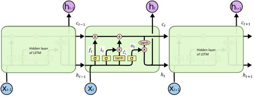
As mentioned earlier, the structure of celled gates enables LSTM to model long-term dependences of sequence data. Gates are served to control cell states of LSTM by allowing information to pass through optionally. There are three types of gates; the input gate, the forget gate, and the output gate denoted by $i_t,$ $f_t,$ $o_t,$ respectively. Values of the cell input state and gates are calculated by Equations (1)–(4). (1) $$i_t={\sigma }_g(W_i{x}_t+U_i{h}_{t-1}+b_i)$$(1) (2) $$f_t={\sigma }_g(W_f{x}_t+U_f{h}_{t-1}+b_f)$$(2) (3) $$o_t={\sigma }_g(W_o{x}_t+U_o{h}_{t-1}+b_o)$$(3) (4) $${\tilde{C}}_t=\tanh (W_c{x}_t+U_o{h}_{t-1}+b_c)$$(4) where $W_i,$ $W_f,$ $W_o,$ $W_c$ denote the weight matrices between the input of the hidden layer, the input gate, the forget gate, the output gate and the input cell state. $U_i,$ $U_f,$ $U_o,$ $U_c$ denote the weight matrices between previous cell output state, input gate, forget gate, output gate and input cell state. $b_i,$ $b_f,$ $b_o,$ $b_c$ denote the corresponding bias vectors.

3.2. Overview of bidirectional LSTM (BDLSTM)

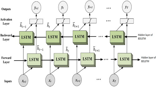
BDLSTM is derived by the idea of bidirectional recurrent neural network (Baldi et al., 1999; Schuster & Paliwal, 1997). In bidirectional recurrent neural network, each training sequence is presented forwards and backwards to two recurrent networks separately, both of which are connected to the same output layer. This means that complete sequential information of all points before or after the given point in sequence data can be retrieved using bidirectional recurrent neural network (Graves & Schmidhuber, 2005). Similarly, in a BDLSTM, sequence data are processed in both directions with forward LSTM and backward LSTM layer and these two hidden layers are connected to the same output layer. A standard topology of BDLSTM is shown in Figure 2 (Yildirim, 2018).

Figure 2. BDLSTM topology.

According to Equations (1)–(4), at each iteration t, cell output state $C_t$ and LSTM layer output $h_t$ are calculated using Equations (5)(5) $$C_t=f_t\mathrm{*}{C}_{t-1}+{{\tilde{C}}_t\mathrm{*}i}_t$$(5) and (6)(6) $$h_t=o_t{\mathrm{*}\tanh (C}_t)$$(6) . (5) $$C_t=f_t\mathrm{*}{C}_{t-1}+{{\tilde{C}}_t\mathrm{*}i}_t$$(5) (6) $$h_t=o_t{\mathrm{*}\tanh (C}_t)$$(6)

BDLSTMs have been applied in the field of trajectory prediction (Xue et al., 2017; Zhao et al., 2018), speech recognition (Zeyer et al, 2017; Zheng et al., 2016), biomedical event analysis (Wang et al., 2017), natural language processing (Xu et al., 2018), traffic speed prediction (Cui & Wang, 2018), etc. It is reported in the literature that BDLSTM outperforms conventional LSTM in some areas such as frame wise phoneme classification (Graves & Schmidhuber, 2005) as well as automatic speech recognition and understanding (Graves et al., 2013).

3.3. Overview of CatBoost

Boosting is an ensemble algorithm that trains and combines weak learners into a strong learner in a systematic manner (Freund & Schapire, 1997). However, pre-processing steps that convert categorical input variables into numeric representations are required by conventional boosting algorithms. For example, one of the most common approaches to pre-process categorical features is one-hot encoding (Micci-Barreca, 2001), which replaces the original categorical feature with binary values for each category. This approach consumes large memory and is computationally intensive, especially when dealing with categorical features of high cardinalities. Another approach to deal with categorical inputs, adopted by the LightGBM algorithm, converts categorical features into gradient statistics at each gradient boosting step. However, this approach results in a high computation cost due to the fact that statistics calculation is performed for each categorical feature at each step (Prokhorenkova et al., 2018).

A more efficient boosting approach, namely categorical boosting (CatBoost) (Dorogush et al., 2018), is proposed to tackle this problem. To be more specific, a modified target-based statistics (TBS) algorithm is used in CatBoost. Assume that dataset $D={\{(X_i,{\mathrm{ }Y}_i)\}\mathrm{ }}_{i=1,\dots ,n},$ where $X_i=(x_{i,1},\dots ,{\mathrm{ }x}_{i,m})$ is a vector consists of both numerical and categorical features, m is the number of features. $Y_i\in \mathrm{Ɍ}$ is the corresponding label. First, the dataset is randomly permutated. Then, for each sample, the average value of the label is calculated for samples with the same category value prior to the given one in the permutation. Let $\sigma ={\sigma }_1,\dots ,{\sigma }_n$ denotes the permutation. Then, the permutated observation $x_{i,\mathrm{k}}$ is replaced with $x_{{\sigma }_{\rho ,}k}\mathrm{ }$ and $x_{{\sigma }_{\rho ,}k}\mathrm{ }$ is calculated by $$\frac{{\sum }_{j=1}^{p-1}\left[x_{{\sigma }_{j,}k}=x_{{\sigma }_{\rho ,}k}\right]Y_{{\sigma }_j}+a.P}{{\sum }_{j=1}^{p-1}\left[x_{{\sigma }_{j,}k}=x_{{\sigma }_{\rho ,}k}\right]+a}.$$ where $\left[x_{j,k}=x_{i,k}\right]$ = 1 if $x_{j,k}=x_{i,k}$ and 0 otherwise. $P$ denotes the prior value and $a$ is the corresponding weight. Prior is the average label value for regression and a priori probability of encountering a positive label for classification. Adding prior serves to reduce the noise from minor categories (Cestnik, 1990). On the one hand, the proposed method utilises the whole dataset for training. On the other hand, it avoids the overfitting problem by performing random permutations.

Moreover, to overcome the biased gradients problems in conventional boosting algorithms (Friedman, 2002), a new schema of calculating leaf values when selecting tree structure is presented in CatBoost. To be more specific, assume $F^i$ denotes the built model and $g^i(X_{k,}{\mathrm{ }Y}_k)$ denotes the gradient value of the k-th training sample after building i trees. To keep the gradient unbiased, for each sample $X_{k,}$ a separate model $M_k$ is trained, which is not updated using a gradient estimate for this sample. The gradient on $X_k$ is estimated using $M_k.$ Then, the resulting tree is scored according to the estimation. Detailed steps of the algorithm are presented in Table 1 (Dorogush et al., 2018).

Table 1. Gradient estimation by CatBoost.

Algorithm: Gradient estimation by CatBoost

Input: training data$\mathrm{ }{\left\{\right(X_k,{\mathrm{ }Y}_k\left)\right\}}_{k=1}^n$ after random permutation, number of trees T, choice loss function$\mathrm{ }\phi (y_j,\mathrm{ }a).$ Initialization: $M_i$ $<-$ for i = 1,…,n Do for iter = 1,…,I  Do for i = 1,…,n   Do for j = 1,…,i-1    $g_j<-\mathrm{ }\frac{d}{da}$ $\phi \left(y_j,a\right){|}_{a=M_i(X_j)}$   $M$ $<-$ BuildOneTree(($X_j,g_j$) for j = 1,…,i-1)   $M_i$ $<-$ $M_i+\mathrm{ }{M}_{}$ Output: $M_1,\dots ,M_n\mathrm{ };\mathrm{ }{M}_1\left(X_1\right),\mathrm{ }{M}_2\left(X_2\right),\dots ,M_n(X_n).$

4. The proposed method and data description

The overall process of the proposed method is shown in Figure 3.

Figure 3. The overall process of the proposed method.

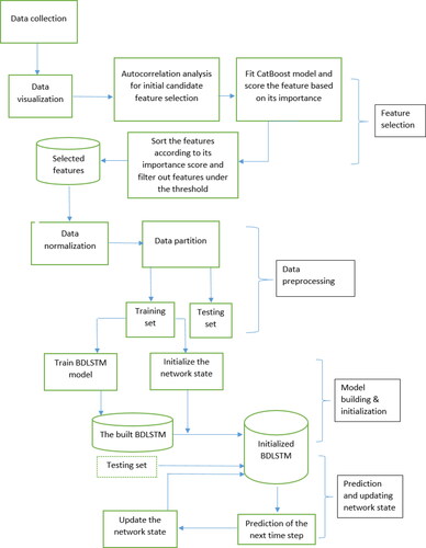
After data collection and visualisation, a two-phase feature selection step is performed. Then, the data are normalised and split in to training and testing set for training and testing the model. Details of the proposed method are discussed in the following subsection. To verify the effectiveness of the proposed method, historical hourly Stockholm electricity price data of Nord Pool market are employed as a case study. Details of the dataset are discussed in the following subsection.

4.1. Data description

Nord Pool (“as of May 19, 2020,” “Nord Pool Website”, 2015) runs the leading power market in Europe with both day ahead and intraday markets being offered. There are four series randomly selected from each season used in this study. Details of each series are shown in Table 2.

Table 2. Details of each series.

Series	Season	Start date	End date	Length
Series 1	Spring	4/11/2018 1:00	5/30/2018 0:00	1200
Series 2	Summer	7/3/2018 9:00	8/22/2018 8:00	1200
Series 3	Autumn	9/10/2018 13:00	10/30/2018 11:00	1200
Series 4	Winter	1/5/2018 5:00	2/24/2018 4:00	1200

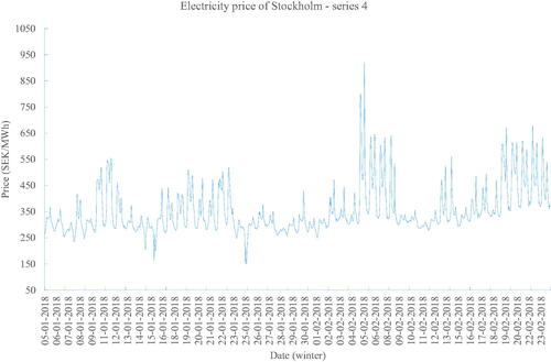
Plots of four series are shown in Figures 4–7, respectively. It can be seen from the plot that series 1 and 3 have greater fluctuation compared with the other two series, while series 2 and 4 present stronger seasonality.

Figure 4. Spring electricity price of Stockholm – series 1.

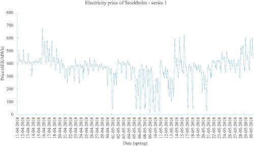
Figure 5. Summer electricity price of Stockholm – series 2.

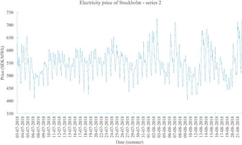
Figure 6. Autumn electricity price of Stockholm – series 3.

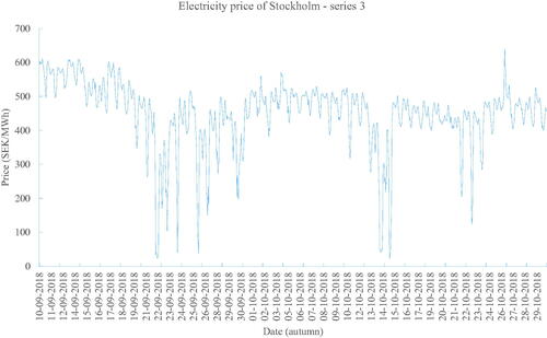
Figure 7. Winter electricity price of Stockholm – series 4.

4.2. The proposed method

After data collection and visualisation, autocorrelation tests of four series data are performed and the corresponding results are plotted in Figures 8–11. The blue areas represent the approximate 95% confidence intervals of autocorrelations. Dots that appear outside the blue area are statistically significant, which indicate potential autocorrelations at a 95% confidence interval.

Figure 8. Autocorrelation plot of series 1.

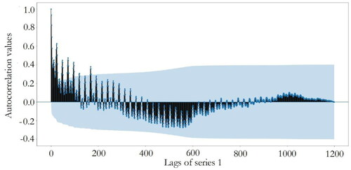
Figure 9. Autocorrelation plot of series 2.

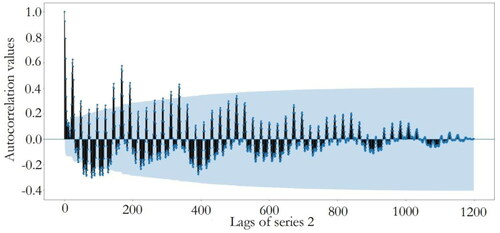
Figure 10. Autocorrelation plot of series 3.

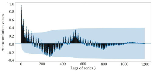
Figure 11. Autocorrelation plot of series 4.

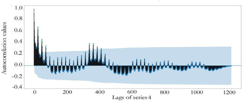
Initial input features are selected from the lags of original series according to Autocorrelation Function (ACF) plots. Apart from numeric features, there are three categorical variables derived from the dataset which are the hour of the day, weekend (the current day is weekend or no), and the day name.

Figures 8–11 show that there exists significant correlation near the 200th lag for series 1 and significant autocorrelation values are observed after the 300th lag in series 2 and 3. For series 4, there is significant correlation near the 400th lag. Therefore, the first 200, 400, 400, and 450 lags of electricity price along with the three categorical features are chosen as the initial candidate features for series one to four, respectively.

To eliminate features that present less useful information for forecasting, the initial candidate features are fed to CatBoost algorithm first. After model fitting, the importance of each feature is calculated by Equation (8)(8) $$\mathrm{Feature}\_\mathrm{importance}\mathrm{ }=\mathrm{ }\sum _{\mathit{trees},\mathrm{ }\mathit{leaves}}{(v_1-\frac{v_1{c}_1+v_2{c}_1}{c_1+c_2})}^2.c_1+{(v_2-\frac{v_1{c}_1+v_2{c}_2}{c_1+c_2})}^2.c_{\mathrm{2\dots }}$$(8) . (8) $$\mathrm{Feature}\_\mathrm{importance}\mathrm{ }=\mathrm{ }\sum _{\mathit{trees},\mathrm{ }\mathit{leaves}}{(v_1-\frac{v_1{c}_1+v_2{c}_1}{c_1+c_2})}^2.c_1+{(v_2-\frac{v_1{c}_1+v_2{c}_2}{c_1+c_2})}^2.c_{\mathrm{2\dots }}$$(8) where $c_1,c_2$ denote the number of samples at a leaf node, while $v_1,v_2$ denote the formula value of the leaf. After the importance score is calculated for each feature, it is sorted from highest to lowest, a threshold score of 0.05 is adopted and features with a lower importance score are filtered out. As a result, there are 123, 136, 156, and 143 features selected for series 1–4, respectively. A full list of selected features and the corresponding importance rankings for each series are presented in Appendix 2.

After feature selection, top rows with NA values are removed. As a result, Series 1 consists of data points from 19 April 2018, 10:00 am to 30 May 2018, 0:00 am. Series 2 consists of data points from 20 July 2018, 2:00 am to 22 August 2018, 8:00 am. Series 3 consists of data points from 27 September 2018, 6:00 am to 30 October 2018, 11:00 am and Series 4 consists of data points from 23 January 2018, 0:00 am to 24 February 2018, 4:00 am, respectively.

Then, data normalisation is performed for by Equation (9)(9) $$x_s=(x-\mathrm{ }\mathrm{\alpha )/\sigma }$$(9) . (9) $$x_s=(x-\mathrm{ }\mathrm{\alpha )/\sigma }$$(9) where $\alpha$ denotes the mean value of the series data and σ denotes the corresponding standard deviation.

The resultant preprocessed data are split, so that 80% of the normalised dataset is used for training and 20% for testing. The experiment is repeated 15 times for each model and initial weights of BDLSTM, GRU, LSTM, and MLP are randomly initialised for each run.

The state of BDLSTM is initialised by predicting on the training data first. After that, to perform the forecasting of n time steps ahead of data points in the testing set, one-time step forecasting approach is used. To be more specific, prediction of the first testing sample is made by the initialised BDLSTM model. Next, the prediction value is utilised to update the network state, after that, the test sample of the next time step is predicted using the updated model. The process is iterated for the remaining time steps to be predicted.

5. Results and discussions

The forecasting results of the proposed BDLSTM together with the other baseline models (SVR, MLP, ARIMA, ensemble tree, GRU, and LSTM) for each series are presented in Figures 12–19.

Figure 12. A plot of the actual price and the predictions by non-deep learning models for series 1.

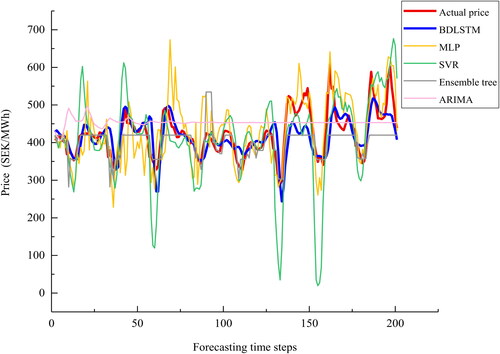
Figure 13. A plot of the actual price and the predictions by deep learning models for series 1.

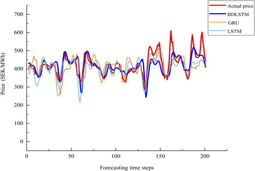
Figure 14. A plot of the actual price and the predictions by non-deep learning models for series 2.

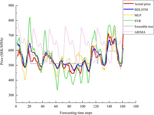
Figure 15. A plot of the actual price and the predictions by deep learning models for series 2.

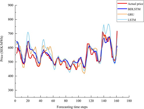
Figure 16. A plot of the actual price and the predictions by non-deep learning models for series 3.

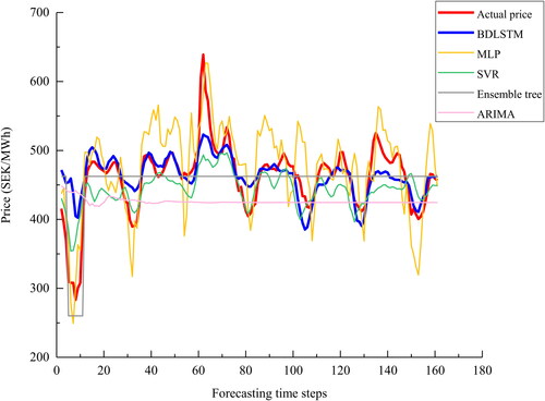
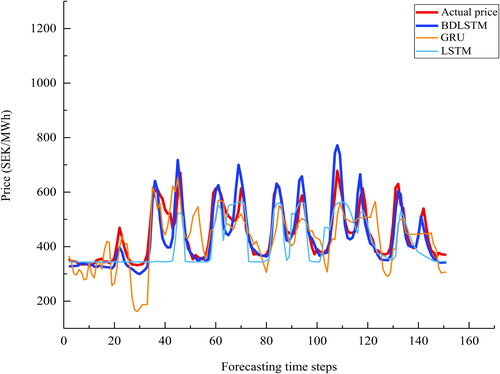
Figure 17. A plot of the actual price and the predictions by deep learning models for series 3.

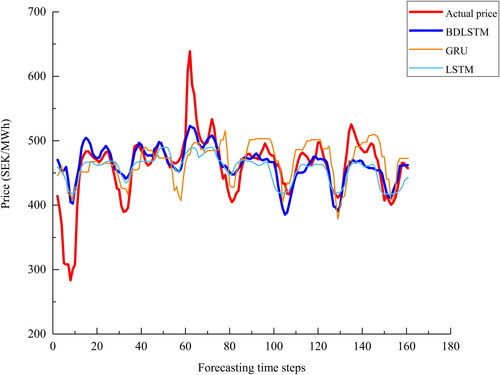
Figure 18. A plot of the actual price and the predictions by non-deep learning models for series 4.

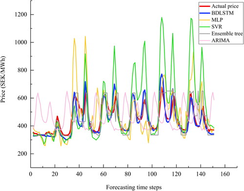
Figure 19. A plot of the actual price and the predictions by deep learning models for series 4.

Series 1: Figures 12 and 13 show that the proposed BDLSTM model captures the overall trend of the original price. Especially from the beginning time step until approximately 130th time step, forecasting values of the proposed model fit the actual electricity price closely. From approximately the 130th time step afterwards, where spikes and valleys are present, the proposed model tends to underestimate the actual values, although the trend is still fully captured by the model. There are two major reasons that contribute to this phenomenon. The first is due to the presence of spikes in the entire series. Spikes are generally caused by certain short-term events or gaming behaviours, which are not the long-term trends of market factors. These events are usually subjective and difficult to forecast (Zhao et al., 2007). Amjady and Keynia (2011) reported that model price spikes, in general, cannot be modelled by conventional electricity price forecast approaches effectively due to the highly erratic behaviours and dependency on complex factors (L. Wang et al., 2017). There are particular studies focussing on the forecasting of electricity price spikes (Amjady & Keynia, 2011; Fragkioudaki et al., 2015; Manner et al., 2016; Sandhu et al., 2016; Voronin & Partanen, 2013). However, forecasting of electricity price spikes is not within the scope of this study and is considered as future work. Another factor is that the one-step ahead forecasting suffers from the problem of error accumulation, as predicted values are served as inputs to predict the next time step (Chevillon, 2007; Ching-Kang, 2003). Overall, the figure shows that the proposed BDLSTM model outperforms the rest.

The plot of MLP shows that trends of certain time steps, e.g., time steps between 38 and 51, are not captured correctly by the model. The curve of actual prices displays a small peak between time steps 38 and 51. However, the curve predicted by MLP shows a small valley. SVR model tends to overestimate peak values and underestimate valleys more than the proposed model, e.g., at around time steps 135 and 152, predicted values of SVR deviate far from actual prices. Ensemble tree outperforms MLP and SVR models. However, predicted values of ensemble tree model are over smoothed, this being more pronounced for series two and three than for series one and four. Therefore, ensemble tree fails to capture the detailed dynamics presented in the series. ARIMA model overestimates for almost all forecasting time steps and predicts constant price after time step 60 approximately. In addition, predictions of GRU model deviate to actual prices at the start and the end of forecasting time steps, while LSTM shows an overall better performance than that of GRU, thought it underestimates the valleys more than BDLSTM.

Series 2: this series contains certain seasonality, but with fewer spikes and valleys than series 1. The proposed model fits the data very well for series 2 as depicted in Figures 14 and 15 with slightly underestimated prediction between time steps 20 and 40 as well as time steps 80 and 100. MLP and SVR overestimate high values as well as underestimate low values. ARIMA predicts a similar seasonality as that is presented in the actual series, though predicted values are overestimated for almost all forecasting time steps. In terms of the forecasting results of deep learning models, LSTM tends to overestimate the peaks, while GRU predictions deviate more from time steps 50 to 60 and the valley at time step 110 is underestimated more by GRU comparing to the other two deep learning models. Due to the presence of spikes and less significant valleys in Series 2 comparing to Series 1, the proposed model tends to overestimate these peak values rather than underestimating valleys.

Series 3: as depicted in Figures 16 and 17, the overall trend is well captured by BDLSTM, however, the same problem of prediction of valleys and spikes remains at approximate time step 9 and 61. MLP underestimates valleys and overestimates peaks of almost the entire series while predictions by ensemble tree remain the same after the 20th time step. The ARIMA suffers from the similar over smoothed problem as ensemble tree does. In addition, GRU model shows a relatively big deviation to the actual price at approximately time step 58, while LSTM underestimates the peak between time step 60 and 70. Overall, the predicted values of the proposed model follow the actual prices more closely than predicted values of the rest models.

Series 4: from Figures 18 and 19, the predicted values of BDLSTM follow the actual prices closely, obvious deviation from the actual prices is not observed for almost all time steps. Besides, the over smoothed problem of ensemble tree and ARIMA is less obvious. It is also observed that forecasted values of ARIMA model display certain seasonality present in the actual electricity prices. However, other dynamics such as trend, peaks, and valleys are not captured properly by ARIMA. This is due to the factor that when complex nonlinearity dynamics are presented in a time series, the performance of ARIMA suffers (Deb et al., 2017). Concerning SVR, the major problem is that it overestimates the peak values of the actual prices most among all models considered. In terms of the performance of deep learning models, except BDLSTM, the other two models suffer to predict the first forecasting time steps. To be more specific, GRU model shows noisy predictions at the first 20 forecasting time steps. On the contrary, LSTM prediction values are over smoothed before the 40 time step. The plots of Series 4 show relatively regular seasonality patterns than the other three series. Therefore, forecasting errors of the proposed model are more evenly distributed instead of showing relatively obvious overestimated or underestimated predictions in certain time steps especially where peaks and valleys are presented as shown in the other three series.

In general, BDLSTM outperforms the other models for all series, SVR and MLP tend to overestimate peaks and underestimate valleys. While predicted values of ensemble tree and ARIMA are over smoothed. Error measures adopted in this study are MAPE, RMSE, and MAE. Apart from the error measurement, training and forecasting time of each model are also measured. Average results are reported in Table 3 and the best run results with least errors of each model are presented in Table 4. Besides, the detailed results of all 15 runs can be found in Appendix 1.

Table 3. Average results of the models for each series.

Measures		BDLSTM	MLP	SVR	ET	ARIMA	GRU	LSTM
Series 1	MAPE	7.113	12.623	14.904	7.728	12.043	9.568	7.496
	RMSE	43.013	67.939	94.611	52.843	67.054	53.866	45.807
	MAE	30.810	52.775	59.684	35.400	54.843	40.921	32.625
	Training time (s)	83.434	5.708	64.187	0.061	121.510	30.600	27.781
	Testing time (s)	3.894	0.046	0.055	0.005	0.020	1.597	1.667
Series 2	MAPE	5.142	8.346	9.720	5.924	19.063	5.778	6.516
	RMSE	37.335	55.853	69.113	40.535	139.367	39.497	45.919
	MAE	27.783	44.270	52.327	32.207	123.796	31.199	35.700
	Training time (s)	88.308	3.001	21.209	0.036	139.430	20.973	18.602
	Testing time (s)	3.568	0.041	0.012	0.005	0.250	1.384	1.259
Series 3	MAPE	5.846	10.348	6.541	6.750	11.956	6.861	6.311
	RMSE	36.885	62.750	37.982	40.978	62.349	41.804	40.300
	MAE	24.485	46.357	29.785	30.415	51.010	29.626	27.067
	Training time (s)	98.062	5.567	63.231	0.081	305.530	30.195	29.968
	Testing time (s)	3.095	0.066	0.078	0.013	0.030	1.107	1.118
Series 4	MAPE	7.742	18.802	23.028	10.491	26.032	14.584	11.786
	RMSE	53.839	117.847	180.574	69.350	147.859	81.226	76.585
	MAE	37.006	86.874	115.979	48.726	122.974	63.061	56.004
	Training time (s)	110.023	9.810	55.130	0.577	187.800	29.974	34.377
	Testing time (s)	3.030	0.035	0.063	0.040	0.240	1.053	1.351

Table 4. The best run of each model for each series.

Measures		BDLSTM	MLP	SVR	ET	ARIMA	GRU	LSTM
Series 1	MAPE	7.015	11.515	14.904	7.728	12.043	9.336	7.325
	RMSE	42.518	60.976	94.611	52.843	67.054	53.306	44.726
	MAE	30.653	48.301	59.684	35.400	54.843	40.564	31.705
	Training time (s)	77.124	6.841	64.187	0.061	121.510	41.547	24.805
	Testing time (s)	3.635	0.037	0.055	0.005	0.020	1.880	1.335
Series 2	MAPE	4.441	6.921	9.720	5.924	19.063	5.740	6.476
	RMSE	31.888	45.397	69.113	40.535	139.367	39.335	45.502
	MAE	23.939	36.144	52.327	32.207	123.796	30.997	35.462
	Training time (s)	89.034	3.165	21.209	0.036	139.430	18.777	16.433
	Testing time (s)	3.525	0.106	0.012	0.005	0.250	1.241	1.218
Series 3	MAPE	5.265	8.095	6.541	6.750	11.956	6.768	6.120
	RMSE	34.993	43.077	37.982	40.978	62.349	40.874	38.907
	MAE	22.186	36.452	29.785	30.415	51.010	29.186	26.318
	Training time (s)	103.724	4.329	63.231	0.081	305.530	31.466	32.760
	Testing time (s)	3.420	0.035	0.078	0.013	0.030	1.087	1.129
Series 4	MAPE	7.137	16.855	23.028	10.491	26.032	14.010	11.059
	RMSE	48.394	111.768	180.574	69.350	147.859	77.315	79.421
	MAE	33.991	77.833	115.979	48.726	122.974	60.697	54.422
	Training time (s)	103.811	6.234	55.130	0.577	187.800	25.248	30.487
	Testing time (s)	3.126	0.036	0.063	0.040	0.240	0.920	1.289

Results show that the proposed model outperforms the other models considered in the experiment for all series for the chosen error measures. The lowest MAPE is achieved by the proposed model with values of 7.015%, 4.441%, 5.265%, and 7.137% for series 1–4, respectively. However, the average time for training the BDLSTM model is higher than for training the other models except ARIMA. Furthermore, the trained BDLSTM is less time efficient in forecasting comparing with the other models. Ensemble tree is the most time efficient model in terms of forecasting efficiency but has lower accuracy. To further compare predictive accuracy, a Diebold–Mariano test (Diebold & Mariano, 2012) is performed. The null hypothesis is that the proposed BDLSTM is as accurate as the other model it is compared with. While the alternative hypothesis is that the model to be compared with is less accurate than BDLSTM. p values of Diebold–Mariano test are reported in Table 5.

Table 5. DM test p values of models to be compared with the proposed BDLSTM for each series.

Series	BDLSTM-MLP	BDLSTM-SVR	BDLSTM-ET	BDLSTM-ARIMA	BDLSTM-GRU	BDLSTM-LSTM
Series 1	4.18E-05	6.70E-06	5.53E-05	1.46E-13	8.26E-06	0.09303
Series 2	1.13E-05	5.72E-08	6.17E-04	<2.2e-16	1.29E-04	1.13E-05
Series 3	0.01191	0.08409	0.02924	4.34E-15	4.21E-06	5.28E-05
Series 4	2.77E-05	3.39E-08	2.39E-03	<2.2e-16	5.03E-06	7.77E-05

Diebold–Mariano test results show that BDLSTM is more accurate than the other models considered in this study for almost all tested series with a significance level of 0.05, apart from Series 3 forecasting result of SVR and Series 1 forecasting result of LSTM. Although the overall errors of BDLSTM reported in Tables 3 and 4 are lower, there is not enough evidence to prove BDLSTM is more accurate than SVR for Series 3 or LSTM for Series 1 with a significance level of 0.05 in this case.

6. Limitations and notes for future researchers

According to the latest review of short-term electricity prices forecasting (Zhang & Fleyeh, 2019), there is a lack of recognised benchmarking procedure and a standard dataset for benchmarking of different models, which make the direct comparison of different results difficult. To be more specific, researchers use different error measures, dataset, length of training/testing time steps, start/end date used, and so forth. To make the future benchmarking procedure easier, the instructions of accessing the dataset used in this study are provided, the dataset can be accessed by the link of Nord Pool (“Nord Pool Historical Market Data”) website in “.xls” format, the filtering criteria used for historical hourly electricity spot prices data retrieve is “Elspot Prices” in the “Filter by category” filter and “Hourly” in the “Filter by resolution” filter. The motivation of the instructions is for the ease of other researchers to access the dataset used in this study and encourage future researchers to use the published dataset for benchmarking or upload their own datasets and provide the instructions of how to access them if possible. In addition, it is advised to use the same error measures, length of training/testing, and other factors involved in the benchmarking procedure.

7. Conclusion and future work

In this article, a novel hybrid model is proposed for short-term electricity price forecasting. It combines a Catboost algorithm for feature selection and BDLSTM neural network model for forecasting. The major advantages of the proposed method are that categorical features are handled more efficiently. Besides, BDLSTM is superior to other methods for modelling complex dependencies inside the series data. The experiment results show that the proposed approach outperforms the other models in terms of MAPE, RMSE, and MAE for series with large fluctuations of electricity prices as well as series with smaller fluctuation but with seasonality present. A limitation of the proposed model is that it consumes more time in terms of both training and forecasting comparing with other models.

There are four suggestions for future studies. Firstly, optimisation techniques such as particle swarm optimisation (PSO), genetic algorithm (GA), differential evolutionary (DE) can be explored to optimise the model structure and parameters such as number of hidden layers, number of neurons as well as the weights of each connection. Secondly, to reduce the accumulated error introduced by the one-step-ahead forecasting approach, other approaches such as training separate models for each time horizon separately using only past observations, multi-step ahead approach can be examined. Besides, electricity price spikes shall be handled more carefully by a separate approach to further improve the forecasting accuracy. Moreover, to enhance time efficiency, graphic processing unit (GPU) and parallel computing techniques can be considered. Finally, instructions of accessing the dataset used in this study are provided, which can be served as a benchmarking dataset for future researchers, suggestions of making future benchmarking procedure smoother are advised as well.

Disclosure statement

No potential conflict of interest was reported by the authors.

Appendix 1.

Results of each run

 

Table

Series 1	Measures	BDLSTM	MLP	SVR	ET	ARIMA	GRU	LSTM
Run 1	MAPE	7.251	12.402	14.904	7.728	12.043	9.776	7.796
	RMSE	41.953	68.613	94.611	52.843	67.054	54.268	47.782
	MAE	31.125	52.159	59.684	35.400	54.843	41.065	34.100
	Training time (s)	77.560	6.199	64.187	0.061	121.510	29.798	32.979
	Testing time (s)	3.943	0.115	0.055	0.005	0.020	1.695	2.373
Run 2	MAPE	7.185	13.882	14.904	7.728	12.043	9.555	7.463
	RMSE	41.619	70.889	94.611	52.843	67.054	54.195	45.910
	MAE	30.858	57.836	59.684	35.400	54.843	41.272	32.343
	Training time (s)	82.033	4.203	64.187	0.061	121.510	33.008	30.782
	Testing time (s)	4.111	0.118	0.055	0.005	0.020	1.642	1.631
Run 3	MAPE	7.023	13.046	14.904	7.728	12.043	9.603	7.489
	RMSE	42.094	71.207	94.611	52.843	67.054	54.107	46.215
	MAE	30.556	53.937	59.684	35.400	54.843	41.355	32.211
	Training time (s)	84.752	4.362	64.187	0.061	121.510	31.720	27.753
	Testing time (s)	3.903	0.035	0.055	0.005	0.020	1.602	1.717
Run 4	MAPE	7.140	13.261	14.904	7.728	12.043	9.428	7.549
	RMSE	44.092	69.825	94.611	52.843	67.054	53.323	45.177
	MAE	30.865	55.050	59.684	35.400	54.843	40.786	32.597
	Training time (s)	89.214	5.873	64.187	0.061	121.510	30.129	28.340
	Testing time (s)	4.075	0.039	0.055	0.005	0.020	1.727	1.564
Run 5	MAPE	7.015	13.473	14.904	7.728	12.043	9.713	7.325
	RMSE	42.518	76.996	94.611	52.843	67.054	54.216	44.726
	MAE	30.653	57.151	59.684	35.400	54.843	40.847	31.705
	Training time (s)	77.124	7.422	64.187	0.061	121.510	28.226	24.805
	Testing time (s)	3.635	0.037	0.055	0.005	0.020	1.349	1.335
Run 6	MAPE	7.127	13.152	14.904	7.728	12.043	9.732	7.590
	RMSE	43.923	70.002	94.611	52.843	67.054	54.191	46.676
	MAE	30.798	54.184	59.684	35.400	54.843	40.838	33.169
	Training time (s)	107.890	6.591	64.187	0.061	121.510	32.107	23.545
	Testing time (s)	3.506	0.037	0.055	0.005	0.020	1.590	1.326
Run 7	MAPE	7.020	11.515	14.904	7.728	12.043	9.811	7.426
	RMSE	42.766	60.976	94.611	52.843	67.054	54.686	45.297
	MAE	30.731	48.301	59.684	35.400	54.843	41.129	32.469
	Training time (s)	78.133	6.841	64.187	0.061	121.510	27.712	25.610
	Testing time (s)	4.609	0.037	0.055	0.005	0.020	1.338	1.566
Run 8	MAPE	7.017	13.009	14.904	7.728	12.043	9.685	7.599
	RMSE	42.301	66.244	94.611	52.843	67.054	53.613	46.211
	MAE	30.602	53.474	59.684	35.400	54.843	40.753	33.279
	Training time (s)	70.649	5.999	64.187	0.061	121.510	29.620	40.839
	Testing time (s)	3.582	0.034	0.055	0.005	0.020	1.426	2.639
Run 9	MAPE	7.109	12.025	14.904	7.728	12.043	9.693	7.374
	RMSE	43.756	66.009	94.611	52.843	67.054	53.756	46.008
	MAE	30.710	50.854	59.684	35.400	54.843	40.780	32.415
	Training time (s)	79.927	6.026	64.187	0.061	121.510	27.090	29.047
	Testing time (s)	3.695	0.034	0.055	0.005	0.020	2.003	1.702
Run 10	MAPE	7.016	12.186	14.904	7.728	12.043	9.688	7.480
	RMSE	42.6144	64.780	94.611	52.843	67.054	54.217	44.430
	MAE	30.682	51.723	59.684	35.400	54.843	41.583	32.547
	Training time (s)	83.245	3.883	64.187	0.061	121.510	28.248	23.349
	Testing time (s)	3.812	0.035	0.055	0.005	0.020	1.414	1.427
Run 11	MAPE	7.134	12.435	14.904	7.728	12.043	9.345	7.547
	RMSE	44.005	64.685	94.611	52.843	67.054	53.312	45.897
	MAE	30.833	51.680	59.684	35.400	54.843	40.585	32.793
	Training time (s)	81.784	6.885	64.187	0.061	121.510	35.776	24.701
	Testing time (s)	3.838	0.034	0.055	0.005	0.020	1.787	1.431
Run 12	MAPE	7.113	11.598	14.904	7.728	12.043	9.336	7.397
	RMSE	43.783	61.035	94.611	52.843	67.054	53.306	45.720
	MAE	30.727	47.708	59.684	35.400	54.843	40.564	32.221
	Training time (s)	90.027	4.168	64.187	0.061	121.510	41.547	24.341
	Testing time (s)	4.229	0.036	0.055	0.005	0.020	1.880	1.444
Run 13	MAPE	7.018	12.145	14.904	7.728	12.043	9.407	7.402
	RMSE	42.715	67.269	94.611	52.843	67.054	54.240	45.925
	MAE	30.713	52.322	59.684	35.400	54.843	40.952	32.166
	Training time (s)	88.046	8.454	64.187	0.061	121.510	27.108	24.902
	Testing time (s)	3.899	0.033	0.055	0.005	0.020	1.787	1.462
Run 14	MAPE	7.298	13.204	14.904	7.728	12.043	9.392	7.518
	RMSE	42.4527	70.181	94.611	52.843	67.054	53.266	46.354
	MAE	31.403	54.226	59.684	35.400	54.843	40.693	32.824
	Training time (s)	83.877	4.139	64.187	0.061	121.510	27.261	27.053
	Testing time (s)	3.728	0.032	0.055	0.005	0.020	1.352	1.795
Run 15	MAPE	7.226	12.434	14.904	7.728	12.043	9.359	7.486
	RMSE	43.650	71.047	94.611	52.843	67.054	53.290	44.781
	MAE	30.896	51.029	59.684	35.400	54.843	40.615	32.541
	Training time (s)	77.248	4.569	64.187	0.061	121.510	27.278	25.697
	Testing time (s)	3.840	0.039	0.055	0.005	0.020	1.369	1.586
Series 2	Measures	BDLSTM	MLP	SVR	ET	ARIMA	GRU	LSTM
Run 1	MAPE	5.362	9.209	9.720	5.924	19.063	5.756	6.483
	RMSE	39.654	59.852	69.113	40.535	139.367	39.407	45.622
	MAE	29.0149	48.222	52.327	32.207	123.796	31.084	35.511
	Training time (s)	92.207	4.149	21.209	0.036	139.430	23.100	18.136
	Testing time (s)	3.498	0.078	0.012	0.005	0.250	1.590	1.503
Run 2	MAPE	5.141	6.921	9.720	5.924	19.063	5.785	6.583
	RMSE	36.484	45.397	69.113	40.535	139.367	39.528	46.306
	MAE	27.922	36.144	52.327	32.207	123.796	31.238	36.067
	Training time (s)	92.971	3.165	21.209	0.036	139.430	21.528	20.349
	Testing time (s)	3.699	0.106	0.012	0.005	0.250	1.250	1.411
Run 3	MAPE	5.256	7.543	9.720	5.924	19.063	5.777	6.536
	RMSE	40.149	49.564	69.113	40.535	139.367	39.497	45.885
	MAE	28.672	40.058	52.327	32.207	123.796	31.197	35.771
	Training time (s)	92.733	2.690	21.209	0.036	139.430	30.059	17.990
	Testing time (s)	3.746	0.031	0.012	0.005	0.250	1.795	1.682
Run 4	MAPE	4.441	7.126	9.720	5.924	19.063	5.769	6.490
	RMSE	31.888	47.238	69.113	40.535	139.367	39.461	45.608
	MAE	23.939	38.231	52.327	32.207	123.796	31.152	35.544
	Training time (s)	89.034	2.642	21.209	0.036	139.430	21.263	19.052
	Testing time (s)	3.525	0.032	0.012	0.005	0.250	1.415	1.112
Run 5	MAPE	5.564	8.663	9.720	5.924	19.063	5.743	6.477
	RMSE	38.994	54.474	69.113	40.535	139.367	39.353	45.511
	MAE	30.145	45.997	52.327	32.207	123.796	31.017	35.468
	Training time (s)	91.293	2.914	21.209	0.036	139.430	20.500	19.394
	Testing time (s)	3.530	0.040	0.012	0.005	0.250	1.273	1.088
Run 6	MAPE	5.481	9.130	9.720	5.924	19.063	5.786	6.476
	RMSE	40.830	61.858	69.113	40.535	139.367	39.533	45.502
	MAE	29.693	48.137	52.327	32.207	123.796	31.244	35.462
	Training time (s)	87.953	3.085	21.209	0.036	139.430	18.944	16.433
	Testing time (s)	3.558	0.036	0.012	0.005	0.250	1.659	1.218
Run 7	MAPE	5.533	8.438	9.720	5.924	19.063	5.795	6.479
	RMSE	39.010	57.199	69.113	40.535	139.367	39.568	45.532
	MAE	29.907	45.957	52.327	32.207	123.796	31.290	35.480
	Training time (s)	92.750	3.001	21.209	0.036	139.430	19.900	20.070
	Testing time (s)	3.148	0.034	0.012	0.005	0.250	1.234	1.661
Run 8	MAPE	4.630	8.880	9.720	5.924	19.063	5.804	6.519
	RMSE	32.034	60.707	69.113	40.535	139.367	39.604	46.010
	MAE	25.053	46.620	52.327	32.207	123.796	31.337	35.722
	Training time (s)	108.316	3.264	21.209	0.036	139.430	20.603	19.031
	Testing time (s)	3.724	0.032	0.012	0.005	0.250	1.258	1.123
Run 9	MAPE	5.315	8.578	9.720	5.924	19.063	5.814	6.537
	RMSE	38.998	57.729	69.113	40.535	139.367	39.639	46.285
	MAE	28.913	46.126	52.327	32.207	123.796	31.386	35.840
	Training time (s)	77.646	3.317	21.209	0.036	139.430	19.752	18.487
	Testing time (s)	3.401	0.031	0.012	0.005	0.250	1.183	1.282
Run 10	MAPE	5.440	7.820	9.720	5.924	19.063	5.773	6.512
	RMSE	38.230	49.604	69.113	40.535	139.367	39.479	46.245
	MAE	29.253	40.955	52.327	32.207	123.796	31.174	35.726
	Training time (s)	91.088	2.627	21.209	0.036	139.430	18.649	16.692
	Testing time (s)	3.827	0.032	0.012	0.005	0.250	1.195	1.080
Run 11	MAPE	4.805	8.652	9.720	5.924	19.063	5.764	6.509
	RMSE	36.702	59.889	69.113	40.535	139.367	39.443	46.187
	MAE	26.159	45.789	52.327	32.207	123.796	31.129	35.713
	Training time (s)	82.747	3.074	21.209	0.036	139.430	18.976	20.238
	Testing time (s)	3.660	0.031	0.012	0.005	0.250	1.423	1.186
Run 12	MAPE	4.874	8.383	9.720	5.924	19.063	5.740	6.594
	RMSE	35.255	56.731	69.113	40.535	139.367	39.335	46.341
	MAE	26.679	45.572	52.327	32.207	123.796	30.997	36.113
	Training time (s)	80.085	2.952	21.209	0.036	139.430	18.777	19.143
	Testing time (s)	3.473	0.030	0.012	0.005	0.250	1.241	1.110
Run 13	MAPE	5.383	7.635	9.720	5.924	19.063	5.803	6.525
	RMSE	38.637	54.648	69.113	40.535	139.367	39.599	45.804
	MAE	29.106	40.665	52.327	32.207	123.796	31.331	35.723
	Training time (s)	84.907	2.658	21.209	0.036	139.430	21.411	17.867
	Testing time (s)	3.710	0.033	0.012	0.005	0.250	1.396	1.156
Run 14	MAPE	4.608	9.041	9.720	5.924	19.063	5.794	6.484
	RMSE	34.151	60.229	69.113	40.535	139.367	39.564	45.673
	MAE	24.791	47.923	52.327	32.207	123.796	31.284	35.534
	Training time (s)	80.371	2.705	21.209	0.036	139.430	21.194	18.044
	Testing time (s)	3.520	0.035	0.012	0.005	0.250	1.267	1.095
Run 15	MAPE	5.294	9.171	9.720	5.924	19.063	5.764	6.535
	RMSE	39.005	62.414	69.113	40.535	139.367	39.443	46.276
	MAE	28.736	47.657	52.327	32.207	123.796	31.129	35.833
	Training time (s)	80.521	2.767	21.209	0.036	139.430	19.941	18.107
	Testing time (s)	3.495	0.036	0.012	0.005	0.250	1.587	1.185
Series 3	Measures	BDLSTM	MLP	SVR	ET	ARIMA	GRU	LSTM
Run 1	MAPE	5.594	8.526	6.541	6.750	11.956	6.854	6.187
	RMSE	36.314	52.068	37.982	40.978	62.349	41.733	40.128
	MAE	23.323	38.293	29.785	30.415	51.010	29.505	26.691
	Training time (s)	76.961	7.577	63.231	0.081	305.530	29.566	27.627
	Testing time (s)	3.582	0.121	0.078	0.013	0.030	1.143	1.108
Run 2	MAPE	5.265	10.483	6.541	6.750	11.956	6.785	6.247
	RMSE	34.993	60.308	37.982	40.978	62.349	41.936	39.971
	MAE	22.186	47.142	29.785	30.415	51.010	29.261	26.708
	Training time (s)	103.724	9.448	63.231	0.081	305.530	29.337	31.340
	Testing time (s)	3.420	0.287	0.078	0.013	0.030	1.059	1.152
Run 3	MAPE	6.013	10.814	6.541	6.750	11.956	6.768	6.173
	RMSE	36.728	75.796	37.982	40.978	62.349	40.874	39.549
	MAE	25.255	47.450	29.785	30.415	51.010	29.186	26.180
	Training time (s)	77.694	4.891	63.231	0.081	305.530	31.466	28.170
	Testing time (s)	3.423	0.078	0.078	0.013	0.030	1.087	1.060
Run 4	MAPE	5.561	9.792	6.541	6.750	11.956	6.875	6.272
	RMSE	36.023	60.202	37.982	40.978	62.349	41.649	40.290
	MAE	23.205	43.382	29.785	30.415	51.010	29.725	26.796
	Training time (s)	111.635	4.552	63.231	0.081	305.530	32.501	33.818
	Testing time (s)	3.431	0.052	0.078	0.013	0.030	1.119	0.266
Run 5	MAPE	5.891	8.486	6.541	6.750	11.956	6.840	6.120
	RMSE	37.611	50.262	37.982	40.978	62.349	41.581	38.907
	MAE	24.435	37.840	29.785	30.415	51.010	29.560	26.318
	Training time (s)	111.123	6.303	63.231	0.081	305.530	27.510	32.760
	Testing time (s)	3.421	0.109	0.078	0.013	0.030	1.055	1.129
Run 6	MAPE	5.520	14.773	6.541	6.750	11.956	6.884	6.305
	RMSE	36.314	97.635	37.982	40.978	62.349	42.072	39.833
	MAE	23.323	65.168	29.785	30.415	51.010	29.765	27.151
	Training time (s)	105.981	3.635	63.231	0.081	305.530	29.543	28.428
	Testing time (s)	3.014	0.036	0.078	0.013	0.030	1.047	1.048
Run 7	MAPE	5.791	9.498	6.541	6.750	11.956	6.858	6.366
	RMSE	32.857	56.517	37.982	40.978	62.349	41.719	40.457
	MAE	24.771	43.881	29.785	30.415	51.010	29.630	27.349
	Training time (s)	94.639	4.861	63.231	0.081	305.530	35.677	27.701
	Testing time (s)	3.086	0.033	0.078	0.013	0.030	1.156	1.111
Run 8	MAPE	6.223	8.095	6.541	6.750	11.956	6.786	6.256
	RMSE	38.789	43.077	37.982	40.978	62.349	41.346	41.010
	MAE	25.910	36.452	29.785	30.415	51.010	29.278	26.938
	Training time (s)	117.600	4.329	63.231	0.081	305.530	30.272	40.093
	Testing time (s)	2.911	0.035	0.078	0.013	0.030	1.055	1.440
Run 9	MAPE	6.263	11.307	6.541	6.750	11.956	6.799	6.232
	RMSE	39.606	65.261	37.982	40.978	62.349	41.863	39.767
	MAE	26.204	50.781	29.785	30.415	51.010	29.397	26.695
	Training time (s)	72.693	5.349	63.231	0.081	305.530	29.433	29.656
	Testing time (s)	2.925	0.034	0.078	0.013	0.030	1.111	1.409
Run 10	MAPE	6.396	9.517	6.541	6.750	11.956	6.894	6.192
	RMSE	40.619	61.943	37.982	40.978	62.349	41.792	39.869
	MAE	26.319	41.474	29.785	30.415	51.010	29.684	26.559
	Training time (s)	111.294	7.613	63.231	0.081	305.530	30.057	28.028
	Testing time (s)	2.958	0.033	0.078	0.013	0.030	1.059	1.445
Run 11	MAPE	6.043	12.722	6.541	6.750	11.956	6.895	6.515
	RMSE	38.278	75.268	37.982	40.978	62.349	41.954	41.564
	MAE	25.211	57.625	29.785	30.415	51.010	29.806	27.674
	Training time (s)	127.059	3.852	63.231	0.081	305.530	32.240	30.137
	Testing time (s)	3.203	0.035	0.078	0.013	0.030	1.455	1.246
Run 12	MAPE	5.903	11.009	6.541	6.750	11.956	6.997	6.444
	RMSE	34.868	65.856	37.982	40.978	62.349	42.726	40.579
	MAE	25.020	50.259	29.785	30.415	51.010	30.244	27.917
	Training time (s)	103.256	4.808	63.231	0.081	305.530	31.087	27.344
	Testing time (s)	1.566	0.036	0.078	0.013	0.030	1.095	1.033
Run 13	MAPE	5.960	11.286	6.541	6.750	11.956	6.919	6.398
	RMSE	38.825	64.926	37.982	40.978	62.349	41.951	41.207
	MAE	25.008	51.258	29.785	30.415	51.010	29.944	27.376
	Training time (s)	82.500	6.414	63.231	0.081	305.530	27.631	26.465
	Testing time (s)	3.353	0.034	0.078	0.013	0.030	1.024	1.100
Run 14	MAPE	5.918	9.323	6.541	6.750	11.956	6.944	6.451
	RMSE	37.577	56.603	37.982	40.978	62.349	42.320	40.577
	MAE	24.615	41.075	29.785	30.415	51.010	29.938	27.659
	Training time (s)	98.518	5.973	63.231	0.081	305.530	27.551	29.185
	Testing time (s)	2.947	0.031	0.078	0.013	0.030	1.067	1.110
Run 15	MAPE	5.349	9.595	6.541	6.750	11.956	6.824	6.513
	RMSE	33.877	55.530	37.982	40.978	62.349	41.537	40.793
	MAE	22.495	43.278	29.785	30.415	51.010	29.463	27.998
	Training time (s)	76.261	3.898	63.231	0.081	305.530	29.055	28.766
	Testing time (s)	3.135	0.039	0.078	0.013	0.030	1.066	1.120

Table

Series 4	Measures	BDLSTM	MLP	SVR	ET	ARIMA	GRU	LSTM
Run 1	MAPE	7.252	19.640	23.028	10.491	26.032	14.381	12.569
	RMSE	54.370	125.606	180.574	69.350	147.859	77.924	81.592
	MAE	35.553	91.320	115.979	48.726	122.974	60.818	60.128
	Training time (s)	119.977	10.212	55.130	0.577	187.800	28.781	35.556
	Testing time (s)	3.075	0.034	0.063	0.040	0.240	0.941	1.427
Run 2	MAPE	7.924	16.855	23.028	10.491	26.032	14.460	11.931
	RMSE	52.578	111.768	180.574	69.350	147.859	82.690	75.818
	MAE	37.648	77.833	115.979	48.726	122.974	64.350	56.497
	Training time (s)	109.587	6.234	55.130	0.577	187.800	24.380	28.139
	Testing time (s)	3.221	0.036	0.063	0.040	0.240	0.918	1.148
Run 3	MAPE	7.590	19.793	23.028	10.491	26.032	15.270	12.490
	RMSE	49.099	125.9820	180.574	69.350	147.859	82.339	78.789
	MAE	35.860	91.513	115.979	48.726	122.974	63.478	59.473
	Training time (s)	124.274	8.441	55.130	0.577	187.800	34.719	29.437
	Testing time (s)	2.829	0.037	0.063	0.040	0.240	1.141	1.399
Run 4	MAPE	7.458	20.072	23.028	10.491	26.032	14.399	11.952
	RMSE	52.891	128.181	180.574	69.350	147.859	82.740	77.964
	MAE	35.582	95.172	115.979	48.726	122.974	64.203	56.585
	Training time (s)	91.418	11.472	55.130	0.577	187.800	39.085	31.682
	Testing time (s)	3.003	0.037	0.063	0.040	0.240	1.169	1.326
Run 5	MAPE	7.273	18.152	23.028	10.491	26.032	14.010	11.956
	RMSE	54.479	105.910	180.574	69.350	147.859	77.315	77.893
	MAE	35.254	82.967	115.979	48.726	122.974	60.697	56.633
	Training time (s)	77.202	10.705	55.130	0.577	187.800	25.248	29.651
	Testing time (s)	2.708	0.033	0.063	0.040	0.240	0.920	1.239
Run 6	MAPE	7.991	19.344	23.028	10.491	26.032	14.425	11.403
	RMSE	53.803	125.347	180.574	69.350	147.859	82.661	62.189
	MAE	37.856	91.670	115.979	48.726	122.974	64.268	50.241
	Training time (s)	122.527	11.343	55.130	0.577	187.800	24.898	32.609
	Testing time (s)	2.954	0.032	0.063	0.040	0.240	0.935	1.298
Run 7	MAPE	8.085	20.557	23.028	10.491	26.032	14.677	11.079
	RMSE	53.650	139.962	180.574	69.350	147.859	79.387	75.206
	MAE	38.033	97.926	115.979	48.726	122.974	61.357	52.918
	Training time (s)	128.976	10.278	55.130	0.577	187.800	24.989	31.539
	Testing time (s)	2.915	0.035	0.063	0.040	0.240	0.877	1.249
Run 8	MAPE	8.109	17.946	23.028	10.491	26.032	14.409	11.059
	RMSE	55.026	115.416	180.574	69.350	147.859	82.667	79.421
	MAE	38.141	83.264	115.979	48.726	122.974	64.233	54.422
	Training time (s)	105.525	10.409	55.130	0.577	187.800	25.181	30.487
	Testing time (s)	3.198	0.034	0.063	0.040	0.240	0.941	1.289
Run 9	MAPE	8.133	19.656	23.028	10.491	26.032	14.933	12.323
	RMSE	58.365	119.022	180.574	69.350	147.859	80.687	84.939
	MAE	38.590	88.215	115.979	48.726	122.974	62.188	59.619
	Training time (s)	124.103	9.300	55.130	0.577	187.800	27.617	34.973
	Testing time (s)	3.166	0.033	0.063	0.040	0.240	1.014	1.274
Run 10	MAPE	7.368	18.177	23.028	10.491	26.032	14.403	12.675
	RMSE	51.634	107.685	180.574	69.350	147.859	82.691	82.545
	MAE	35.422	81.236	115.979	48.726	122.974	64.219	60.988
	Training time (s)	127.177	12.366	55.130	0.577	187.800	29.299	32.992
	Testing time (s)	2.984	0.035	0.063	0.040	0.240	1.147	1.185
Run 11	MAPE	7.811	19.696	23.028	10.491	26.032	15.123	11.221
	RMSE	55.960	120.794	180.574	69.350	147.859	81.642	70.841
	MAE	37.749	91.777	115.979	48.726	122.974	62.891	52.985
	Training time (s)	94.126	7.921	55.130	0.577	187.800	32.511	35.030
	Testing time (s)	3.101	0.033	0.063	0.040	0.240	1.017	1.228
Run 12	MAPE	8.221	18.538	23.028	10.491	26.032	15.395	11.254
	RMSE	58.076	117.018	180.574	69.350	147.859	82.893	73.384
	MAE	40.160	85.953	115.979	48.726	122.974	63.984	53.782
	Training time (s)	114.562	11.701	55.130	0.577	187.800	27.833	31.705
	Testing time (s)	3.071	0.034	0.063	0.040	0.240	1.025	1.288
Run 13	MAPE	7.137	16.917	23.028	10.491	26.032	14.397	11.636
	RMSE	48.394	97.428	180.574	69.350	147.859	82.753	74.358
	MAE	33.991	75.131	115.979	48.726	122.974	64.188	55.077
	Training time (s)	103.811	10.875	55.130	0.577	187.800	27.284	36.359
	Testing time (s)	3.126	0.035	0.063	0.040	0.240	1.080	1.313
Run 14	MAPE	8.027	19.568	23.028	10.491	26.032	14.014	11.722
	RMSE	55.787	117.765	180.574	69.350	147.859	77.311	75.743
	MAE	38.305	89.523	115.979	48.726	122.974	60.695	55.367
	Training time (s)	108.258	9.624	55.130	0.577	187.800	48.686	51.857
	Testing time (s)	2.920	0.035	0.063	0.040	0.240	1.248	1.732
Run 15	MAPE	7.760	17.125	23.028	10.491	26.032	14.459	11.524
	RMSE	53.476	117.958	180.574	69.350	147.859	82.690	78.094
	MAE	36.947	79.607	115.979	48.726	122.974	64.349	55.343
	Training time (s)	98.819	6.267	55.130	0.577	187.800	29.098	43.634
	Testing time (s)	3.174	0.037	0.063	0.040	0.240	1.425	1.871

Appendix 2.

A full list of features selected and ranked by Catboost for each series

 

Table

Series 1		Series 2		Series 3		Series 4
Feature	Score	Feature	Score	Feature	Score	Feature	Score
Lag_1	36.187	Lag_1	4.565	Lag_1	23.709	Lag_1	18.710
Lag_2	10.670	Lag_366	3.352	Lag_2	3.694	Lag_3	3.248
Lag_4	5.556	Lag_43	3.192	Lag_297	3.190	Lag_166	2.732
Lag_22	1.986	Lag_197	3.036	Lag_27	2.583	Lag_45	2.341
Lag_100	1.875	Lag_162	2.647	Lag_304	2.190	Lag_418	2.132
Lag_3	1.845	Lag_321	2.607	Lag_11	2.114	Lag_385	2.122
Lag_70	1.465	Lag_160	2.152	Lag_308	1.862	Lag_361	2.002
Lag_29	1.419	Lag_102	2.065	Lag_352	1.653	Lag_386	1.979
Lag_20	1.323	Lag_25	2.037	Lag_5	1.541	Lag_25	1.974
Lag_23	1.317	Lag_371	2.019	Lag_339	1.469	Lag_431	1.971
Lag_19	1.248	Lag_205	2.009	Lag_36	1.386	Lag_237	1.744
Lag_96	1.168	Lag_34	1.984	Lag_44	1.234	Lag_17	1.701
Lag_121	1.004	Lag_168	1.948	Lag_346	1.222	Lag_55	1.610
Lag_143	0.967	Lag_12	1.880	Lag_254	1.215	Lag_24	1.562
Lag_114	0.920	Lag_252	1.598	Lag_102	1.195	Lag_287	1.552
Lag_199	0.882	Lag_84	1.597	Lag_61	1.162	Lag_382	1.500
Lag_181	0.775	Lag_128	1.586	Lag_155	1.112	Lag_243	1.396
Weekend	0.757	Lag_204	1.567	Lag_163	1.101	Lag_2	1.300
Lag_57	0.732	Lag_264	1.542	Lag_77	1.098	Lag_392	1.132
Lag_136	0.689	Lag_378	1.523	Lag_152	1.085	Lag_376	1.016
Lag_84	0.664	Lag_337	1.472	Lag_121	1.082	Lag_186	0.952
Lag_193	0.635	Lag_16	1.463	Lag_128	1.053	Lag_108	0.945
Lag_196	0.618	Lag_99	1.434	Lag_97	1.052	Lag_407	0.928
Lag_150	0.610	Lag_304	1.412	Lag_64	1.050	Lag_20	0.921
Lag_24	0.609	Lag_338	1.375	Lag_3	1.047	Lag_387	0.899
Lag_105	0.591	Lag_369	1.329	Lag_150	0.950	Lag_403	0.869
Lag_123	0.588	Lag_152	1.136	Lag_199	0.941	Lag_36	0.851
Lag_78	0.583	Lag_263	1.128	Lag_189	0.919	Lag_249	0.830
Lag_102	0.565	Lag_309	1.085	Lag_96	0.884	Lag_354	0.814
Lag_71	0.563	Lag_120	1.068	Lag_49	0.881	Lag_142	0.778
Lag_63	0.558	Lag_90	1.047	Lag_188	0.859	Lag_336	0.762
Lag_37	0.551	Lag_227	1.009	Lag_342	0.816	Lag_424	0.759
Lag_21	0.543	Lag_301	0.996	Lag_131	0.807	Lag_200	0.751
Lag_39	0.538	Day_name	0.983	Lag_361	0.798	Lag_22	0.739
Lag_25	0.528	Lag_146	0.978	Lag_154	0.791	Lag_6	0.736
Lag_124	0.519	Lag_399	0.943	Lag_309	0.768	Lag_218	0.726
Lag_191	0.519	Lag_379	0.798	Lag_146	0.740	Lag_288	0.722
Lag_75	0.505	Lag_54	0.775	Lag_187	0.717	Lag_423	0.651
Lag_73	0.503	Lag_27	0.775	Lag_172	0.695	Lag_359	0.638
Lag_58	0.475	Lag_96	0.772	Lag_386	0.666	Lag_193	0.626
Lag_178	0.461	Lag_312	0.761	Lag_114	0.659	Lag_435	0.608
Lag_92	0.456	Lag_397	0.747	Lag_360	0.586	Lag_196	0.602
Lag_16	0.422	Lag_344	0.744	Lag_84	0.532	Lag_168	0.600
Lag_88	0.420	Lag_13	0.731	Lag_250	0.525	Lag_132	0.596
Lag_194	0.418	Lag_315	0.721	Lag_213	0.523	Lag_135	0.594
Lag_155	0.417	Lag_218	0.706	Lag_10	0.488	Lag_75	0.574
Lag_99	0.393	Lag_222	0.698	Lag_282	0.485	Lag_81	0.571
Lag_129	0.330	Lag_360	0.691	Lag_255	0.481	Lag_107	0.569
Lag_145	0.320	Lag_88	0.660	Lag_333	0.471	Lag_257	0.563
Lag_158	0.316	Lag_2	0.644	Lag_171	0.469	Lag_319	0.560
Lag_9	0.296	Lag_83	0.635	Lag_24	0.456	Lag_377	0.560
Lag_149	0.289	Lag_216	0.630	Lag_385	0.452	Lag_201	0.556
Lag_43	0.285	Lag_288	0.629	Lag_383	0.450	Lag_158	0.544
Lag_195	0.273	Lag_194	0.618	Lag_370	0.446	Lag_16	0.533
Lag_7	0.271	Weekend	0.614	Lag_319	0.444	Lag_371	0.529
Lag_46	0.265	Lag_62	0.609	Lag_223	0.433	Lag_267	0.503
Lag_160	0.263	Lag_343	0.591	Lag_151	0.420	Lag_139	0.501
Lag_139	0.260	Lag_295	0.572	Lag_235	0.408	Lag_19	0.495
Lag_54	0.252	Lag_181	0.554	Lag_263	0.402	Lag_335	0.477
Lag_168	0.248	Lag_247	0.550	Lag_244	0.400	Lag_337	0.457
Lag_60	0.248	Lag_4	0.541	Lag_148	0.370	Lag_406	0.456
Lag_126	0.238	Lag_141	0.523	Lag_265	0.369	Lag_416	0.442
Lag_161	0.232	Lag_3	0.519	Lag_191	0.369	Lag_429	0.426
Lag_132	0.230	Lag_109	0.507	Lag_95	0.365	Lag_270	0.425
Lag_15	0.223	Lag_318	0.485	Lag_382	0.360	Lag_390	0.417
Lag_55	0.222	Lag_319	0.468	Lag_224	0.358	Lag_198	0.408
Lag_45	0.210	Lag_89	0.451	Lag_17	0.330	Lag_26	0.404
Lag_134	0.210	Lag_336	0.448	Lag_216	0.329	Lag_50	0.395
Lag_200	0.205	Lag_182	0.445	Lag_332	0.320	Lag_246	0.386
Lag_101	0.201	Lag_81	0.442	Lag_260	0.314	Lag_419	0.370
Lag_125	0.197	Lag_21	0.440	Lag_203	0.303	Lag_179	0.364
Lag_174	0.197	Lag_275	0.434	Lag_214	0.302	Lag_195	0.362
Lag_11	0.188	Lag_20	0.425	Lag_62	0.297	Lag_316	0.351
Lag_197	0.186	Lag_266	0.422	Lag_190	0.289	Lag_197	0.341
Lag_190	0.183	Lag_243	0.419	Lag_51	0.282	Lag_271	0.333
Lag_127	0.181	Lag_228	0.398	Lag_335	0.281	Lag_272	0.329
Lag_59	0.170	Lag_316	0.392	Lag_115	0.272	Lag_71	0.323
Lag_156	0.169	Lag_17	0.380	Lag_313	0.264	Lag_410	0.320
Lag_27	0.169	Lag_223	0.368	Lag_262	0.258	Lag_189	0.317
Lag_164	0.167	Lag_111	0.366	Lag_176	0.227	Lag_5	0.311
Lag_86	0.164	Lag_287	0.365	Lag_178	0.227	Lag_310	0.285
Lag_189	0.163	Lag_154	0.363	Lag_124	0.224	Lag_236	0.281
Lag_94	0.157	Lag_289	0.335	Lag_167	0.222	Lag_432	0.280
Lag_52	0.150	Lag_200	0.333	Lag_158	0.221	Lag_356	0.272
Lag_5	0.148	Lag_80	0.326	Lag_159	0.216	Lag_263	0.269
Lag_173	0.132	Lag_302	0.321	Lag_30	0.214	Lag_23	0.255
Lag_165	0.126	Lag_199	0.319	Weekend	0.206	Lag_302	0.251
Lag_98	0.123	Lag_69	0.312	Lag_381	0.201	Lag_66	0.246
Lag_198	0.123	Lag_140	0.303	Lag_271	0.198	Lag_433	0.241
Lag_89	0.117	Lag_334	0.288	Lag_100	0.192	Lag_342	0.234
Lag_72	0.115	Lag_157	0.272	Lag_253	0.186	Lag_175	0.220
Lag_69	0.115	Lag_6	0.258	Lag_391	0.182	Lag_293	0.217
Lag_26	0.113	Lag_229	0.246	Lag_85	0.176	Lag_174	0.213
Lag_159	0.110	Lag_171	0.246	Lag_292	0.175	Lag_116	0.213
Lag_192	0.109	Lag_226	0.240	Lag_303	0.170	Lag_347	0.211
Lag_66	0.104	Lag_56	0.209	Lag_34	0.159	Lag_338	0.209
Lag_163	0.103	Lag_377	0.209	Lag_168	0.157	Lag_411	0.192
Lag_188	0.101	Lag_208	0.208	Lag_279	0.152	Lag_163	0.176
Lag_166	0.090	Lag_49	0.199	Lag_29	0.148	Lag_136	0.174
Lag_110	0.089	Lag_361	0.198	Lag_246	0.145	Lag_192	0.173
Lag_162	0.088	Lag_272	0.183	Lag_98	0.140	Lag_11	0.171
Lag_122	0.086	Lag_246	0.173	Lag_228	0.139	Lag_37	0.171
Lag_113	0.081	Lag_63	0.163	Lag_268	0.138	Lag_210	0.171
Lag_87	0.079	Lag_325	0.161	Lag_22	0.137	Lag_73	0.158
Lag_12	0.075	Lag_270	0.159	Lag_166	0.133	Lag_350	0.154
Lag_85	0.073	Lag_306	0.147	Lag_384	0.132	Lag_33	0.153
Lag_144	0.073	Lag_350	0.132	Lag_53	0.125	Lag_262	0.142
Lag_167	0.072	Lag_8	0.131	Lag_353	0.122	Lag_29	0.140
Lag_128	0.069	Lag_14	0.124	Lag_107	0.119	Lag_96	0.140
Lag_81	0.067	Lag_370	0.123	Lag_306	0.116	Lag_279	0.139
Lag_40	0.067	Lag_41	0.123	Lag_270	0.116	Lag_273	0.139
Lag_6	0.066	Lag_330	0.118	Lag_336	0.116	Lag_41	0.136
Lag_82	0.065	Lag_40	0.112	Lag_157	0.115	Lag_63	0.133
Lag_172	0.063	Lag_207	0.108	Lag_379	0.114	Lag_164	0.132
Lag_14	0.063	Lag_237	0.104	Lag_194	0.112	Lag_276	0.128
Lag_28	0.062	Lag_85	0.104	Lag_234	0.110	Lag_94	0.126
Lag_77	0.062	Lag_188	0.103	Lag_4	0.110	Lag_68	0.123
Day_name	0.059	Lag_322	0.094	Lag_233	0.110	Lag_10	0.122
Lag_79	0.059	Lag_283	0.093	Lag_174	0.109	Lag_172	0.118
Lag_50	0.058	Lag_354	0.090	Lag_31	0.109	Lag_225	0.117
Lag_30	0.052	Lag_213	0.078	Lag_32	0.106	Lag_9	0.117
Lag_179	0.051	Lag_55	0.077	Lag_239	0.104	Lag_14	0.114
Lag_10	0.051	Lag_176	0.074	Lag_298	0.098	Lag_123	0.113
		Lag_329	0.071	Lag_142	0.095	Lag_274	0.112
		Lag_145	0.070	Lag_149	0.095	Lag_321	0.112
		Lag_192	0.070	Lag_192	0.095	Lag_89	0.112
		Lag_339	0.069	Lag_217	0.094	Lag_397	0.111
		Lag_47	0.066	Lag_273	0.092	Lag_49	0.099
		Lag_28	0.064	Lag_321	0.092	Lag_183	0.098
		Lag_126	0.064	Lag_278	0.092	Lag_205	0.095
		Lag_364	0.058	Lag_396	0.085	Lag_101	0.083
		Lag_23	0.054	Lag_251	0.083	Lag_150	0.083
		Lag_286	0.054	Lag_369	0.079	Lag_122	0.083
		Lag_273	0.053	Lag_119	0.078	Lag_111	0.083
		Lag_311	0.052	Lag_141	0.078	Lag_85	0.080
		Lag_7	0.050	Lag_305	0.077	Lag_204	0.080
				Lag_329	0.076	Lag_74	0.075
				Lag_106	0.074	Lag_360	0.070
				Lag_113	0.074	Lag_213	0.070
				Lag_221	0.073	Lag_340	0.060
				Lag_165	0.073	Lag_389	0.054
				Lag_104	0.068	Lag_126	0.053
				Lag_72	0.066	Lag_64	0.050
				Lag_318	0.061
				Lag_45	0.059
				Lag_236	0.059
				Lag_83	0.059
				Lag_280	0.058
				Lag_212	0.057
				Lag_238	0.057
				Lag_359	0.056
				Lag_290	0.054
				Lag_259	0.053
				Lag_41	0.052
				Lag_25	0.052
				Lag_120	0.051

References

- Amjady, N., & Keynia, F. (2011). A new prediction strategy for price spike forecasting of day-ahead electricity markets. Applied Soft Computing Journal, 11(6), 4246–4256. https://doi.org/https://doi.org/10.1016/j.asoc.2011.03.024
- Anbazhagan, S., & Kumarappan, N. (2013). Day-ahead deregulated electricity market price forecasting using recurrent neural network. Systems Journal, IEEE, 7(4), 866–872. https://doi.org/https://doi.org/10.1109/JSYST.2012.2225733
- Baldi, P., Brunak, S., Frasconi, P., Soda, G., & Pollastri, G. (1999). Exploiting the past and the future in protein secondary structure prediction. Bioinformatics, 15(11), 937–946. https://doi.org/https://doi.org/10.1093/bioinformatics/15.11.937
- Barnes, P. M. (2017). The politics of nuclear energy in the European Union: Framing the discourse. Barbara Budrich Publishers.
- Bengio, Y., Simard, P., & Frasconi, P. (1994). Learning long-term dependencies with gradient descent is difficult. IEEE Transactions on Neural Networks, 5(2), 157–166. https://doi.org/https://doi.org/10.1109/72.279181
- Berglund, S. (2009). Putting politics into perspective: A study of the implementation of EU public utilities directives. Eburon Uitgeverij B.V., 2009 – European Union countries.
- Cabero, J., Baillo, A., Cerisola, S., Ventosa, M., Garcia-Alcalde, A., Peran, F., & Relano, G. (2005). A medium-term integrated risk management model for a hydrothermal generation company. IEEE Transactions on Power Systems, 20(3), 1379–1388. https://doi.org/https://doi.org/10.1109/TPWRS.2005.851934
- Cestnik, B. (1990). Estimating probabilities: A crucial task in machine learning. In ECAI’90: Proceedings of the 9th European Conference on Artificial Intelligence January (pp. 147–149).
- Chen, T., Carlos, G. (2016). XGBoost: A Scalable Tree Boosting System. In Publication:KDD ’16: Proceedings of the 22nd ACM SIGKDD International Conference on Knowledge Discovery and Data Mining August (pp. 785–794). https://doi.org/https://doi.org/10.1145/2939672.2939785
- Chevillon, G. (2007). Direct multi-step estimation and forecasting. Journal of Economic Surveys, 21(4), 746–785. https://doi.org/https://doi.org/10.1111/j.1467-6419.2007.00518.x
- Ching-Kang, I. (2003). Multistep prediction in autoregressive processes. Econometric Theory, 19(02), 254–279. https://doi.org/https://doi.org/10.1017/S0266466603192031
- Cho, K., van Merrienboer, B., Gulcehre, C., Bahdanau, D., Bougares, F., Schwenk, H., Bengio, Y. (2014). Learning phrase representations using RNN encoder-decoder for statistical machine translation. http://arxiv.org/abs/1406.1078
- Cui, Z., & Wang, Y. (2018). Deep stacked bidirectional and unidirectional LSTM recurrent neural network for network-wide traffic speed prediction. In 23rd ACM SIGKDD conference on knowledge discovery and data mining (KDD) (pp. 22–25). New York, NY, United States: Association for Computing Machinery.
- Deb, C., Zhang, F., Yang, J., Eang, S., & Wei, K. (2017). A review on time series forecasting techniques for building energy consumption. Renewable and Sustainable Energy Reviews, 74(February), 902–924. https://doi.org/https://doi.org/10.1016/j.rser.2017.02.085
- Diebold, F. X., & Mariano, R. S. (2012). Comparing predictive accuracy. Journal of Business & Economic Statistics, 13(3), 253–263. https://doi.org/https://doi.org/10.1080/07350015.1995.10524599
- Dorogush, A. V., Ershov, V., & Gulin, A. (2018). CatBoost: Gradient boosting with categorical features support, arXiv:1810.11363.
- Fragkioudaki, A., Marinakis, A., & Cherkaoui, R. (2015). Forecasting price spikes in European day-ahead electricity markets using decision trees. International Conference on the European Energy Market, EEM, 2015-August. https://doi.org/https://doi.org/10.1109/EEM.2015.7216672
- Freund, Y., & Schapire, R. (1997). A decision-theoretic generalization of on-line learning and an application to boosting. Journal of Computer and System Sciences, 55(1), 119–139. https://doi.org/https://doi.org/10.1006/jcss.1997.1504
- Friedman, J. H. (2002). Stochastic gradient boosting. Computational Statistics & Data Analysis, 38(4), 367–378. https://doi.org/https://doi.org/10.1016/S0167-9473(01)00065-2
- Girish, G. P., & Vijayalakshmi, S. (2015). Role of energy exchanges for power trading in India. International Journal of Energy Economics and Policy, 5(3), 673–676.
- Graves, A., & Schmidhuber, J. (2005). Framewise phoneme classification with bidirectional LSTM and other neural network architectures. Neural Networks: The Official Journal of the International Neural Network Society, 18(5-6), 602–610. https://doi.org/https://doi.org/10.1016/j.neunet.2005.06.042
- Graves, A., Jaitly, N., & Mohamed, A. (2013). Hybrid speech recognition with Deep Bidirectional LSTM. In 2013 IEEE Workshop on Automatic Speech Recognition and Understanding (pp. 273–278). https://doi.org/https://doi.org/10.1109/ASRU.2013.6707742
- Hochreiter, S. (1991). Untersuchungen zu dynamischen neuronalen netzen. Diploma, Technische Universitat Munchen.
- Hochreiter, S., & Schmidhuber, J. (1997). Long short-term memory. Neural Computation, 9(8), 1735–1780. https://doi.org/https://doi.org/10.1162/neco.1997.9.8.1735
- Ke, G., Meng, Q., Finley, T., Wang, T., Chen, W., Ma, W., Ye, Q., & Liu, T. (2017). LightGBM: A highly efficient gradient boosting decision tree. In NIPS’17: Proceedings of the 31st International Conference on Neural Information Processing Systems (pp. 3149–3157). Curran Associates Inc.
- Kuo, P.-H., & Huang, C.-J. (2018). An electricity price forecasting model by hybrid structured deep neural networks. Sustainability, 10(4), 1280. https://doi.org/https://doi.org/10.3390/su10041280
- Lago, J., De Ridder, F., & De Schutter, B. (2018). Forecasting spot electricity prices: Deep learning approaches and empirical comparison of traditional algorithms. Applied Energy, 221(February), 386–405. https://doi.org/https://doi.org/10.1016/j.apenergy.2018.02.069
- Manner, H., Türk, D., & Eichler, M. (2016). Modeling and forecasting multivariate electricity price spikes. Energy Economics, 60, 255–265. https://doi.org/https://doi.org/10.1016/j.eneco.2016.10.006
- Micci-Barreca, D. (2001). A preprocessing scheme for high-cardinality categorical attributes in classification and prediction problems. ACM SIGKDD Explorations Newsletter, 3(1), 27–32. https://doi.org/https://doi.org/10.1145/507533.507538
- Mirikitani, D., & Nikolaev, N. (2011). Nonlinear maximum likelihood estimation of electricity spot prices using recurrent neural networks. Neural Computing and Applications, 20(1), 79–89. https://doi.org/https://doi.org/10.1007/s00521-010-0344-1
- Nord Pool Historical Market Data. (n.d.). Nord Pool. Retrieved November 5, 2020, from https://www.nordpoolgroup.com/historical-market-data/
- Nord Pool Website. (2015). Nord Pool. Retrieved November 5, 2020, from https://www.nordpoolgroup.com/
- Olah, C. (2015). Understanding LSTM networks. Retrieved November 5, 2020, from http://colah.github.io/posts/2015-08-Understanding-LSTMs/
- Pandey, N., & Upadhyay, K. G. (2016). Different price forecasting techniques and their application in deregulated electricity market: A comprehensive study. 2016 International Conference on Emerging Trends in Electrical Electronics & Sustainable Energy Systems (ICETEESES) (pp. 1–4). https://doi.org/https://doi.org/10.1109/ICETEESES.2016.7581342
- Pezzutto, S., Grilli, G., Zambotti, S., & Dunjic, S. (2018). Forecasting electricity market price for end users in EU28 until 2020—Main factors of influence. Energies, 11(6), 1418–1460. https://doi.org/https://doi.org/10.3390/en11061460
- Prokhorenkova, L., Gusev, G., Vorobev, A., Dorogush, A. V., & Gulin, A. (2018). CatBoost: Unbiased boosting with categorical features. In NIPS'18: Proceedings of the 32nd International Conference on Neural Information Processing Systems, December 2018 (pp. 6639–6649). ACM.
- Sandhu, H. S., Fang, L., & Guan, L. (2016). Forecasting day-ahead price spikes for the Ontario electricity market. Electric Power Systems Research, 141, 450–459. https://doi.org/https://doi.org/10.1016/j.epsr.2016.08.005
- Schuster, M., & Paliwal, K. K. (1997). Bidirectional recurrent neural networks. IEEE Transactions on Signal Processing, 45(11), 2673–2681. https://doi.org/https://doi.org/10.1109/78.650093
- Sulehria, H. K., & Zhang, Y. (2007). Hopfield neural networks: A survey. In AIKED’07 Proceedings of the 6th Conference on 6th WSEAS Int. Conf. on Artificial Intelligence, Knowledge Engineering and Data Bases (Vol. 6, pp. 125–130).
- Ugurlu, U., Oksuz, I., & Tas, O. (2018). Electricity price forecasting using recurrent neural networks. Energies, 11(5), 1255. https://doi.org/https://doi.org/10.3390/en11051255
- Vardhan, N. H., & Chintham, V. (2015). Electricity price forecasting of deregulated market using Elman neural network. In 2015 Annual IEEE India Conference (INDICON) (pp. 1–5). https://doi.org/https://doi.org/10.1109/INDICON.2015.7443460
- Ventosa, M., Baı́llo, Á., Ramos, A., & Rivier, M. (2005). Electricity market modeling trends. Energy Policy, 33(7), 897–913. https://doi.org/https://doi.org/10.1016/j.enpol.2003.10.013
- Voronin, S., & Partanen, J. (2013). Price forecasting in the day-ahead energy market by an iterative method with separate normal price and price spike frameworks. Energies, 6(11), 5897–5920. https://doi.org/https://doi.org/10.3390/en6115897
- Wang, L., Member, S., Zhang, Z., & Chen, J. (2017). Short-term electricity price forecasting with stacked denoising autoencoders. IEEE Transactions on Power Systems, 32(4), 2673–2681. https://doi.org/https://doi.org/10.1109/TPWRS.2016.2628873
- Wang, Y., Wang, J., Lin, H., Zhang, S., & Li, L. (2017). Biomedical event trigger detection based on bidirectional LSTM and CRF. In 2017 IEEE International Conference on Bioinformatics and Biomedicine (BIBM) (pp. 445–450). https://doi.org/https://doi.org/10.1109/BIBM.2017.8217689
- Weron, R. (2014). Electricity price forecasting: A review of the state-of-the-art with a look into the future. International Journal of Forecasting, 30(4), 1030–1081. https://doi.org/https://doi.org/10.1016/j.ijforecast.2014.08.008
- Xu, C., Xie, L., & Xiao, X. (2018). A bidirectional LSTM approach with word embeddings for sentence boundary detection. Journal of Signal Processing Systems, 90(7), 1063–1075. https://doi.org/https://doi.org/10.1007/s11265-017-1289-8
- Xue, H. Q., Huynh, D., & Reynolds, M. (2017). Bi-prediction: Pedestrian trajectory prediction based on bidirectional LSTM classification. In 2017 International Conference on Digital Image Computing: Techniques and Applications (DICTA) (pp. 1–8). https://doi.org/https://doi.org/10.1109/DICTA.2017.8227412
- Yildirim, Ö. (2018). A novel wavelet sequence based on deep bidirectional LSTM network model for ECG signal classification. Computers in Biology and Medicine, 96(March), 189–202. https://doi.org/https://doi.org/10.1016/j.compbiomed.2018.03.016
- Zeyer, A., Doetsch, P., Voigtlaender, P., & Schlüter, R. (2017). A comprehensive study of deep bidirectional LSTM RNNS for acoustic modeling in speech recognition. In 2017 IEEE International Conference on Acoustics, Speech and Signal Processing (ICASSP) (pp. 2462–2466). https://doi.org/https://doi.org/10.1109/ICASSP.2017.7952599
- Zhang, F., & Fleyeh, H. (2019). A review of single artificial neural network models for electricity spot price forecasting. In 2019 16th International Conference on the European Energy Market (EEM) (pp. 1–6). https://doi.org/https://doi.org/10.1109/EEM.2019.8916423
- Zhao, J. H., Dong, Z. Y., Li, X., & Wong, K. P. (2007). A framework for electricity price spike analysis with advanced data mining methods. IEEE Transactions on Power Systems, 22(1), 376–385. https://doi.org/https://doi.org/10.1109/TPWRS.2006.889139
- Zhao, Y., Yang, R., Chevalier, G., Shah, R. C., & Romijnders, R. (2018). Optik applying deep bidirectional LSTM and mixture density network for basketball trajectory prediction. Optik – International Journal for Light and Electron Optics, 158, 266–272. https://doi.org/https://doi.org/10.1016/j.ijleo.2017.12.038
- Zheng, D., Chen, Z., Wu, Y., & Yu, K. (2016). Directed automatic speech transcription error correction using bidirectional LSTM. In 2016 10th International Symposium on Chinese Spoken Language Processing (ISCSLP) (pp. 1–5). https://doi.org/https://doi.org/10.1109/ISCSLP.2016.7918446