ATM cash replenishment under varying population coverage requirements

Abstract

Inspired by an automated teller machine (ATM) cash replenishment problem involving population coverage requirements (PCRs) in the Netherlands, we propose the vehicle tour problem with minimum coverage requirements. In this problem, a set of minimum-cost routes is constructed subject to constraints on the duration of each route and the population coverage of the replenished ATMs. A compact formulation incorporating a family of valid inequalities and an efficient tour-splitting metaheuristic are proposed and tested on 77 instances derived from real-life data involving up to 98 ATMs and 237,604 citizens and on 144 newly generated synthetic instances. Our results for the real-life instances indicate significant cost differences in replenishing ATMs for seven major Dutch cities when the PCRs vary. Additionally, we illustrate the impact of different PCRs on the ATM replenishment costs for seven major cities in the Netherlands by presenting an aggregated cost evaluation of 11 PCRs involving 1,003,519 citizens, 338 ATMs, and 19 cash distribution vehicles.

Keywords:

• Covering tour problems
• cash logistics
• networks
• service level requirements
• metaheuristics

1. Introduction

Service level requirements (SLRs) are widely used in supply chain logistics but have received little attention in the academic literature on optimising distribution problems. For example, Lin and Yang (2011) address the design of public bicycle systems both from a user’s and an investor’s viewpoint. The service level provided to users is measured by the demand coverage level and travel costs, while the setup costs for bike stations and bike lanes are considered in the case of the investor. Escalona et al. (2015) develop an inventory location model for the design of a distribution network for fast-moving items able to provide differentiated service levels in terms of product availability for two demand classes (high and low priority) using a critical level policy. Hensher and Houghton (2004) use SLRs to ensure that bus operators deliver service levels consistent with stakeholder needs, especially with the objectives of the Australian government. Recently, Ibarra-Rojas et al. (2014) studied the trade-off between the level of service in the bus network and operating costs incurred (related to fleet size) in Monterrey, while Sawik (2015) deals with a supplier selection and scheduling problem to optimise the expected costs and customer service levels under disruption risks. Zhang et al. (2018) define a service level as the probability of satisfying uncertain demand in build–operate–transfer projects. This service level is imposed by the government on the private firm so that capacity and stochastic demand can be better matched in public transport projects. Moons et al. (2019) provide a recent review measuring, among others, the logistics performance in distributing internal hospital supplies while determining the desired SLRs. The literature on service level considerations in vehicle routing is scarce with the notable exception of Bulhões et al. (2018) who investigate a capacitated routing problem minimising the sum of transportation costs and lost profits subject to strictly non-violated SLRs for groups of customers. Lai (2004) empirically studies different types of service providers and their performance under different SLRs. For an extended and more general overview of the several key performance indicators for logistics service providers, see Krauth et al. (2005).

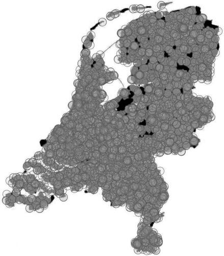
Our research is motivated by a real-life automated teller machine (ATM) cash replenishment problem involving an SLR imposed by the Dutch Central Bank (DNB) through the National Forum on the Payment System to Geldmaat.¹ Cash payments represent the most dominant payment instrument in a large majority of sectors throughout Europe. In recent years, however, digital or contactless payments have become widely available (2017). This trend has caused the gradual removal of ATMs in many European countries (2018). The accessibility of the public to ATMs and to cash in general has recently received public and political attention in the Netherlands. The high operational and maintenance costs of ATMs combined with the reduced used of cash led the banks to remove 6.4% of the ATMs in the country between 2014 and 2017. Despite the increasing use of digital currencies (2018), cash payments still enjoy a high acceptance rate, and their use is unlikely to significantly decline in the next few years (2018). Accessibility also remains an issue, especially for those groups of the population that are less mobile and that often live in rural communities where ATM coverage is low (2017). According to DNB guidelines, Geldmaat has to ensure that 99.73% of the Dutch population has access to a replenished ATM within five kilometres. Figure 1 maps the ATM population coverage in the Netherlands for 2017 when all ATMs are replenished.

Figure 1. ATM population coverage map in the Netherlands for 2017. Black areas represent postal codes with residents not having access to an ATM within five kilometres.

The problem of operating an ATM network subject to population coverage requirements (PCRs) is closely related to the multi-vehicle covering tour problem (m-CTP) first introduced by Hachicha et al. (2000). The m-CTP is a well-known decision-making problem with must-visit and may-visit locations and a set of demand points that must be covered by the visited locations. The m-CTP seeks a set of minimum-cost routes passing through a subset of the locations subject to (i) visiting all must-visit locations, (ii) constraints on the length of each route, (iii) constraints on the number of visited locations on each route, and (iv) covering all demand points by visiting locations within a specific distance. The m-CTP (and its variants) has numerous applications, including the construction of routes for mobile healthcare teams such that all population centres are within a short traveling distance (Hodgson et al., 1998) and in the design of postal box installations maximising an appropriate linear combination of user convenience and postal service efficiency (Labbé & Laporte, 1986). Nevertheless, the m-CTP requires that all demand points are covered, thus implying mandatory 100% coverage.

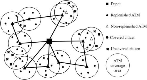
In this article, we introduce the vehicle tour problem with minimum coverage requirements (VTPMCR) capable of handling coverage requirements lower than or equal to 100%. To the best of our knowledge, this is the first study to examine the impact of such coverage requirements on network operating costs. Figure 2 provides an example illustrating a feasible solution of the VTPMCR with coverage strictly lower than 100%, showing that the presence of uncovered citizens makes such a solution infeasible to the m-CTP. The VTPMCR generalises the m-CTP when it comes to the coverage constraints by allowing partial demand point coverage and therefore belongs to the class of NP-hard problems. As a solution to the VTPMCR satisfies coverage requirements and operational constraints, it indicates which ATMs to replenish and provides insights on how to redesign the network, i.e. which ATMs to keep or close.

Figure 2. Example of a feasible solution of the VTPMCR involving uncovered citizen demand and coverage strictly lower than 100%; such a solution is infeasible for the m-CTP.

The main contributions of this study are various. First, we introduce the VTPMCR, a new decision-making problem with applications to various distribution settings. Second, we propose a compact formulation and incorporate a family of valid inequalities that allows us to solve real-life instances with up to 50 ATMs and 163,029 citizens to optimality. Third, we propose a tour-splitting metaheuristic for the VTPMCR that can find high-quality solutions for real-life instances with up to 98 ATMs and 237,604 citizens within short computation times. Additionally, we illustrate the cost impact of different PCRs on the ATM replenishment costs for seven major cities in the Netherlands and present an aggregated cost evaluation of 11 PCRs involving 1,003,519 citizens from seven cities, 338 ATMs, and 19 cash distribution vehicles. Finally, we introduce 144 new synthetic problem instances, and we report a computational study indicating how the problem’s main parameters affect the computational behaviour of the proposed solution approaches.

The rest of the article is organised as follows. Section 2 reviews the state–of–the–art on exact and heuristic algorithms for the m-CTP and its main variants. The VTPMCR is formally introduced in Section 3, along with a flow-based formulation for the problem. Section 4 describes the tour-splitting metaheuristic along with nine local search operators incorporated into our solution framework. Section 5 elaborates on the synthetic and the real-life banknote distribution instances and discusses the computational results obtained. Finally, conclusions and future research directions are outlined in Section 6.

2. Literature review

Based on the objective function and constraints, vehicle routing problems (VRPs) can be categorised into classes of problems with special characteristics. m-CTP extend the traditional VRP literature by considering must-visit and may-visit locations and a set of demand points that can be assumed to be covered if a visited location is within a specific distance. Additionally, covering tour problems incorporate constraints on the length of each route and on the number of visited locations per route. When all these modeling aspects are present, the problem under consideration is the m-CTP introduced in Section 1.

2.1. Literature on the m-CTP

Many researchers have studied the m-CTP since its first appearance in the seminal work of Hachicha et al. (2000), who propose three heuristic solution approaches. The first two, namely modified savings and modified sweep algorithms, are based on successful solution approaches for the VRP and vehicle dispatch problem (see Clarke & Wright, 1964 and Gillett & Miller, 1974). The third one follows a route-first cluster-second approach creating a possibly infeasible giant tour that is then split into multiple feasible routes. All three heuristics are tested on two sets of synthetic and real-life instances with up to 200 must-visit/may-visit locations.

Lopes et al. (2013) propose the first exact solution approach for the m-CTP. In particular, the authors propose a Branch-and-Price (BP) algorithm and a column generation heuristic incorporating specific dominance and extension pruning rules to accelerate the resolution of the related pricing problems. Following the guidelines in (2000) for creating 15 instances, the authors solve five instances with up to 50 must-visit/may-visit locations to optimality.

Jozefowiez (2014) proposes a path-based model and a BP algorithm to select routes such that all demand points are covered and all must-visit locations are visited. The constraints associated with the number of visited locations, the number of routes, and their duration are considered in the subproblem based on the integer programming formulation of Labbé et al. (2004). The algorithm can solve 47 out of 80 synthetic instances with up to 60 must-visit/may-visit locations and 150 demand points to optimality.

Finally, a capacitated version of the m-CTP (m-CTP-c) is introduced by Murakami (2018). The capacity constraints for each vehicle reduce to the constraints on the number of visited locations per route when each must-visit/may-visit location is assigned a demand level of one. The authors present a heuristic solution framework which is based on a column generation algorithm, where the route generation problems (subproblems) are solved by applying a heuristic for the CTP. Computational results on a newly generated set of synthetic instances with up to 500 must-visit/may-visit locations and 2500 demand points show the competitiveness of the heuristic by outperforming the three heuristics of Hachicha et al. (2000).

2.2. Literature on variants of the m-CTP

Several studies have explored variants of the m-CTP. Tricoire et al. (2012) consider a Bi-objective Stochastic CTP (bi-SCTP) that aims to minimise the opening cost of distribution centres and incurred transportation costs. The authors develop a Branch-and-Cut (BC) algorithm for a two-stage stochastic optimisation in which the demand of a set of population nodes is stochastic and can be partially covered based on their distance from the visiting distribution centres and present computational results on a set of real-life instances.

A CTP for the location of satellite distribution centres to supply humanitarian aid to affected people throughout a disaster area (CTLSDC) is proposed by Naji-Azimi et al. (2012). In this problem, a heterogeneous and capacitated fleet serves individual demand points with different types of required aid by visiting (possibly multiple times) a set of satellite distribution centres. Neither must-visit locations nor route duration constraints for the vehicles are taken into account in this study. A multi-start heuristic is proposed to produce high-quality solutions for realistically sized instances in reasonable computation times.

Hà et al. (2013) consider a special case of the m-CTP without any restriction on the duration of the routes (m-CTP-p). A new formulation extending that found in Baldacci et al. (2005) for the single-vehicle version of the m-CTP is proposed along with a BC and a metaheuristic solution framework. Competitive computational results on a set of instances with up to 100 must-visit/may-visit and 100 demand points indicate the efficiency of their methods.

Inspired by humanitarian logistics scenarios, Flores-Garza et al. (2017) consider a variant of the m-CTP with the objective of minimising the sum of arrival times (latency) at each visited location (m-CCTP). A mixed integer linear programming formulation and a greedy randomised adaptive search procedure are developed and tested on an adaptation of the 96 instances proposed by Ha et al. (2013).

Kammoun et al. (2017) study the m-CTP-p of Ha et al. (2013). A variable neighbourhood search heuristic based on variable neighbourhood descent is proposed and tested on a set of synthetic instances generated according to the guidelines in (2013).

Pham et al. (2017) develop a BC algorithm and a genetic algorithm adapted from Vidal et al. (2014) for the Multi-vehicle Multi-CTP (mm-CTP) in which the number of vehicles is represented as a variable, the demand points may need to be covered multiple times, and must-visit/may-visit locations may allow for multiple visits. The genetic algorithm outperforms the results of Hà et al. (2013), especially on large instances.

Finally, Karaoğlan et al. (2018) introduce the Multi-vehicle Probabilistic CTP (m-PCTP) whose objective function aims to maximise the expected coverage of the demand points without considering any must-visit locations. A variable neighbourhood search metaheuristic is used to improve the initial solution of a BC algorithm that can solve 538 out of 587 synthetic instances to optimality involving up to 161 may-visit locations and 322 demand points.

Table 1 provides an overview of the different covering tour problems addressed in the literature as well as their corresponding features and references. The table shows that the VTPMCR faced by Geldmaat has not been addressed in the literature yet.

Table 1. A summary of the features of the m-CTP and its main variants: superscripts indicate whether an exact (E) or a metaheuristic (H) solution approach was used; superscripts indicate mandatory full coverage (F) or partial coverage (P).

		Must-visit	Demand point	Constraints			Homogeneous
Acronym	Reference(s)	Locations	Coverage	Capacity	Cardinality	Max duration	Fleet	Objective function
m-CTP	[11]^H, [24]^E, [16]^E	✓	✓^F	✘	✓	✓	✓	Min cost
m-CTP-c	[26]^H	✓	✓^F	✓	✓	✓	✓	Min cost
m-CTP-p	[10]^E,H, [17]^H	✓	✓^F	✘	✓	✘	✓	Min cost
m-CCTP	[8]^H	✓	✓^F	✘	✘	✓	✓	Min sum of arrival times
mm-CTP	[29]^E,H	✓	✓^F	✓	✓	✘	✓	Min cost
m-PCTP	[18]^E	✘	✓^F	✘	✘	✓	✓	Max expected demand covered
bi-SCTP	[33]^E	✘	✘	✓	✓	✘	✘	Min (cost + exp. uncovered demand)
CTLSDC	[27]^H	✘	✓^F	✓	✓	✘	✘	Min distance
VTPMCR	This paper	✘	✓^P	✘	✘	✓	✓	Min cost

3. Problem description

The VTPMCR can be defined on a directed graph $G=(V,A).$ The vertex set $V=\left\{0\right\}\cup S$ represents a depot, 0, and a set $S=\{1,2,\dots ,n\}$ of n ATMs. The set of ATMs can be visited and replenished by up to m vehicles. The arc set A is defined as $A=\{(i,j)|i,j\in V:i\ne j\}.$ Given a set of citizens C that the ATMs can cover, the VTPMCR consists of determining a set of at most m minimum-cost routes on a subset of V, subject to constraints on the maximum route duration T of each route and on the total population coverage of the replenished ATMs of all routes. Specifically, feasible solutions require covering at least P out of $\left|C\right|$ citizens. A citizen $c\in C$ is considered to be covered if there exists at least one replenished (i.e. visited) ATM within a (straight) distance r. Such a distance r, hereafter referred to as the service radius, is defined based on the population density and number of ATMs in the geographical area served. In the following, $S_c\subseteq S$ denotes the set of ATMs that can cover citizen $c\in C,$ and c_ij represents the cost of traveling from i to j, where $(i,j)\in A.$ Motivated by our real-life case, each arc cost c_ij, $(i,j)\in A,$ is set equal to $$c_{ij}=\{\begin{array}{cc}{t}_{ij}+t_r\hfill & \text{if}\mathrm{ }j\in S\hfill \\ t_{ij}\hfill & \text{otherwise}\hfill \end{array}$$ with t_ij representing the time required to travel from $i\in V$ to $j\in V$ and t_r is the fixed replenishment time per ATM. In this study, traveling times are calculated based on real-road distances and a fixed vehicle speed depending on the average distance between the set of ATMs and depot.

Moreover, let $\mathbb{P}=\{{\Phi }_1,{\Phi }_2,\dots ,{\Phi }_{\left|\mathbb{P}\right|}\}$ be a partition of the citizens such that $S_c=S_{c\prime }$ for each pair of citizens $c,c\prime \in C,c\ne c\prime ,$ belonging to the same subset ${\Phi }_k,k=1,\dots ,\left|\mathbb{P}\right|,$ i.e. the two citizens can be served by the same subset of ATMs. Each subset of the partition $\mathbb{P}$ is called family of citizens (or simply family), and we refer to each class corresponding to subset ${\Phi }_k,k=1,\dots ,\left|\mathbb{P}\right|,$ by its index k. Moreover, let $S({\Phi }_k)\subseteq S$ be the subset of ATMs that serve the citizens of the subset ${\Phi }_k$ – i.e. $S({\Phi }_k)=S_c$ for each $c\in {\Phi }_k.$

To formulate the VTPMCR, we introduce three sets of variables:

• $y_k\in \{0,1\}$ is a binary variable equal to 1 if family $k=1,\dots ,\left|\mathbb{P}\right|$ is covered (0 otherwise),

• $x_{ij}\in \{0,1\}$ is a binary variable equal to 1 if any vehicle traverses arc $(i,j)\in A$ (0 otherwise), and

• $z_{ij}\in {\mathbb{R}}_{+}$ is a continuous variable indicating the departure time from i to j, where $i\in S,j\in V.$

The VTPMCR can then be formulated as follows: (1a) $$\min \sum _{(i,j)\in A}{c}_{ij}{x}_{ij}$$(1a) (1b) $$\mathrm{s}.\mathrm{t}.\sum _{k=1}^{\left|\mathbb{P}\right|}\left|{\Phi }_k\right|y_k\ge P$$(1b) (1c) $$\sum _{(i,j)\in A\mathrm{ }:\mathrm{ }j\in S({\Phi }_k)}{x}_{ij}\ge y_k\forall k=1,\dots ,\left|\mathbb{P}\right|$$(1c) (1d) $$\sum _{(0,j)\in A}{x}_{0j}\le m$$(1d) (1e) $$\sum _{(i,j)\in A}{x}_{ij}-\sum _{(j,i)\in A}{x}_{ji}=0\hspace{1em}\forall j\in V$$(1e) (1f) $$\sum _{(i,j)\in A}{x}_{ij}\le 1\forall j\in S$$(1f) (1g) $$z_{ij}\le (\mathrm{T}-t_{ij}-t_{j0})x_{ij}\forall i\in S,\forall j\in V$$(1g) (1h) $$\sum _{(i,j)\in A}{z}_{ij}\ge t_{0i}\sum _{(j,i)\in A}{x}_{ji}\forall i\in S$$(1h) (1i) $$\sum _{(i,j)\in A}(z_{ij}+t_{ij}{x}_{ij})\le \sum _{(j,i)\in A}{z}_{ji}\forall j\in S$$(1i) (1j) $$y_k\in \{0,1\}\forall k=1,\dots ,\left|\mathbb{P}\right|$$(1j) (1k) $$x_{ij}\in \{0,1\}\forall (i,j)\in A$$(1k) (1l) $$z_{ij}\in {\mathbb{R}}_{+}\forall i\in S,\forall j\in V$$(1l)

The objective function (1a)(1a) $$\min \sum _{(i,j)\in A}{c}_{ij}{x}_{ij}$$(1a) minimises the total ATM cash replenishment costs. Constraint (1b)(1b) $$\mathrm{s}.\mathrm{t}.\sum _{k=1}^{\left|\mathbb{P}\right|}\left|{\Phi }_k\right|y_k\ge P$$(1b) guarantees that at least P citizens are covered. Constraints (1c)(1c) $$\sum _{(i,j)\in A\mathrm{ }:\mathrm{ }j\in S({\Phi }_k)}{x}_{ij}\ge y_k\forall k=1,\dots ,\left|\mathbb{P}\right|$$(1c) make sure that a family of citizens is covered only if there is a replenished ATM within the service radius r. Constraints (1d)(1d) $$\sum _{(0,j)\in A}{x}_{0j}\le m$$(1d) limit the number of routes. Constraints (1e)(1e) $$\sum _{(i,j)\in A}{x}_{ij}-\sum _{(j,i)\in A}{x}_{ji}=0\hspace{1em}\forall j\in V$$(1e) are flow conservation constraints. Constraints (1f)(1f) $$\sum _{(i,j)\in A}{x}_{ij}\le 1\forall j\in S$$(1f) make sure that each ATM is visited at most once. Constraints (1g)(1g) $$z_{ij}\le (\mathrm{T}-t_{ij}-t_{j0})x_{ij}\forall i\in S,\forall j\in V$$(1g) define the maximum route duration constraints per vehicle by setting a limit on the maximum departure time from each ATM $i\in S;$ if the arc x_ij is not used, the value of z_ij is equal to 0. Constraints (1h)(1h) $$\sum _{(i,j)\in A}{z}_{ij}\ge t_{0i}\sum _{(j,i)\in A}{x}_{ji}\forall i\in S$$(1h) set the minimum value for z_ij. Constraints (1i)(1i) $$\sum _{(i,j)\in A}(z_{ij}+t_{ij}{x}_{ij})\le \sum _{(j,i)\in A}{z}_{ji}\forall j\in S$$(1i) are flow constraints for the z_ij variables. Finally, constraints (1j)–(1l) define the domain of the variables.

The linear relaxation of formulation (1a)–(1l) can be strengthened with the following set of valid inequalities: (2) $$y_k\ge \sum _{(i,j)\in A}{x}_{ij}\hspace{1em}\forall k=1,\dots ,\left|\mathbb{P}\right|,\mathrm{\hspace{1em}}\mathrm{\hspace{1em}}\forall j\in S({\Phi }_k)$$(2)

These inequalities become active when at least one ATM $j\in S({\Phi }_k)$ being within a service radius r from citizens of family $k=1,\dots ,\left|\mathbb{P}\right|$ is replenished; in that case, variable y_k is forced to take a positive value.

4. A tour-splitting metaheuristic

In this section, we present a route-first cluster-second metaheuristic for the VTPMCR accompanied by iterated local search. The metaheuristic is inspired by tour-splitting approaches proposed for different VRPs. In such approaches, one giant tour visiting all service points (or customers) is created, which is then split into feasible routes. Prins et al. (2009) describe how to improve tour-splitting approaches to obtain better solutions or tackle additional constraints while a recent review recalling the basic route-first cluster-second approach to show how it can efficiently be embedded in constructive heuristics and metaheuristics can be found in the recent work of Prins et al. (2014). In opposite approaches, namely cluster-first split-second approaches, clusters of service points compatible with vehicle capacity are first formed and then optimised by solving the related traveling salesman problems for each cluster to extract higher-quality solutions.

4.1. Overview of the proposed metaheuristic

Algorithm 1.

Overview of the proposed tour-splitting metaheuristic TSMheu

Input: VTPMCR input data

Parameters: ${\overline{\eta }}_0,\hspace{0.5em}{\overline{\eta }}_1,\hspace{0.5em}{\overline{\eta }}_2$

Output: a set of routes $\mathcal{X}=(R_1,\dots ,R_m)$

1: $\mathcal{X}\leftarrow \varnothing ,\hspace{0.5em}c(\mathcal{X})\leftarrow \infty$

2: for ${\eta }_0=1,\dots ,{\overline{\eta }}_0$ do

3:  $\mathcal{S}\leftarrow$ SelectSPs()      ⊳ see Algorithm 2

4:  for ${\eta }_1=1,\dots ,{\overline{\eta }}_1$ do

5:   $\mathcal{T}\leftarrow$ CreateGiantTour($\mathcal{S}$)

6:   for ${\eta }_2=1,\dots ,{\overline{\eta }}_2$ do

7:     $\mathcal{T}\leftarrow$ LocalSearch($\mathcal{T}$) ⊳ see Algorithm 3

8:     $\mathcal{T}\leftarrow$ DeleteSPs($\mathcal{T}$)

9:     $\mathcal{R}\leftarrow$ Split($\mathcal{T}$)

10:     $\mathcal{R}\leftarrow$ LocalSearch($\mathcal{R}$)

11:     if $c(\mathcal{X})>c(\mathcal{R})$ then

12:      $\mathcal{X}\leftarrow \mathcal{R}$

13:     end if

14:     $\mathcal{T}\leftarrow$ CreateGiantTour($S_{\mathcal{R}}$)

15:   end for

16:  end for

17: end for

18: return $\mathcal{X}$

Algorithm 1 provides a pseudocode description of the proposed tour-splitting metaheuristic (TSMheu). The input of the TSMheu is the input data for the VTPMCR. The best solution found by the TSMheu after ${\overline{\eta }}_0$ iterations is indicated by $\mathcal{X},$ where $\mathcal{X}=(R_1,\dots ,R_m)$ denotes the set of m routes forming a feasible solution given a VTPMCR input instance. The two main tasks of the problem, namely ATM selection and the design of minimum-cost routes subject to maximum route duration constraints and minimum PCRs, are carried out sequentially. In each iteration, the $\mathit{selectSPs}$ function selects a set of ATMs that satisfy the minimum PCRs (Line 3). In the following, $\mathcal{P}(\mathcal{S})$ denotes the total number of citizens covered by a set of ATMs $\mathcal{S}\subseteq S.$ Algorithm 2 describes the $\mathit{selectSPs}$ function more in detail.

The ATM selection task is accomplished in a way that, in each of the ${\overline{\eta }}_0$ iterations, a variety of different sets of ATMs is selected. Specifically, in each step of the ATM selection procedure, an equal probability of selection is given to every ATM $i\in S$ with a positive coverage contribution given a set of already selected ATMs $\mathcal{S}$ (i.e. $\mathcal{P}(\mathcal{S}\cup i)-\mathcal{P}(\mathcal{S})>0$). The equal probability of selecting ATMs with positive coverage contribution guarantees that in each iteration of the metaheuristic, a diverse set of ATMs is selected.

Then, for ${\overline{\eta }}_1$ iterations, a giant tour $\mathcal{T}$ is created by iteratively inserting the ATMs of the set $\mathcal{S}$ one by one in the same order as they were selected by the $\mathit{selectSPs}$ function in the position of $\mathcal{T}$ that minimises the cost added to the objective function (Line 5).

The following steps are then applied for a number of ${\overline{\eta }}_2$ iterations. First, an attempt to further optimise $\mathcal{T}$ is made by applying two intra-route operators (Line 7). Second, the ATMs that contribute the most to the objective function value are sequentially removed as long as the minimum PCR is not violated (Line 8). Third, the optimal splitting of $\mathcal{T}$ into a set of routes $\mathcal{R}$ respecting the order of the ATMs in $\mathcal{T}$ is executed (Line 9); such a splitting is cost-driven and aims to minimise the cost of the routes generated from the giant tour; however, the maximum route duration constraints are neglected, meaning that some routes may be infeasible. To address this issue of having infeasible routes and guide the search toward feasible solutions, a penalty factor p is embedded into the cost of each set of routes $\mathcal{R}$ to proportionally penalise the violation of the maximum route duration constraints in the routes. The optimal split of the giant tour $\mathcal{T}$ into a set of minimum-cost routes $\mathcal{R}$ while respecting their order in $\mathcal{T}$ is based on the guidelines of Prins et al. (2009) for VRPs with limited size fleets.

The routes in $\mathcal{R}$ are optimised by a set of nine local search intra- and inter-route operators until no further improvement can be found (Line 10). The solution is then checked, and if it is better than the previous best, it is stored in memory. Finally, the ATMs $S_{\mathcal{R}}$ present in $\mathcal{R}$ are reconnected into a single giant tour $\mathcal{T}$ using the same process as applied in Line 5.

Algorithm 2.

selectSPs()

Input: VTPMCR input data

Output: A set of SPs $\mathcal{S}\subseteq S$ with $\mathcal{P}(\mathcal{S})\ge P$

1: $\mathcal{S}\leftarrow \varnothing$

2: do

3:  Select randomly a SP $i\in S$ with $\mathcal{P}(\mathcal{S}\cup \{i\})>\mathcal{P}(\mathcal{S})$

4:  $\mathcal{S}\leftarrow \mathcal{S}\cup \left\{i\right\}$

5: While $\mathcal{P}(\mathcal{S})<P$

6: return $\mathcal{S}$

4.2. Local search

Algorithm 3 describes the local search procedure (LocalSearch) applied at each iteration of the TSMheu. The input is a (possibly infeasible) solution represented as a set of routes $\mathcal{H},$ and the output is the set of routes obtained after the evaluation of a set of local search moves. The local search procedure is repeated as long as the incumbent solution improves with any of the local search moves.

The local search procedure of the TSMheu consists of three improving components: intra-route, inter-route, and population coverage improvement. All three components may affect the value of the objective function. The population coverage, however, can only be differentiated by the operators incorporated in the population coverage improvement component. Overall, nine local search operators are applied, of which seven deal with route improvement and two with population coverage improvement: (1) swap-intra (i.e. exchanging the positions of two ATMs on a single route), (2) 2-opt-intra (i.e. the well-known 2-opt applied within a single route), (3) 2-0-relocate-inter (i.e. relocating two consecutive ATMs of a route to another route), (4) 2-1-exchange-inter (i.e. exchanging two consecutive ATMs of a route with an ATM of another route), (5) swap-inter (i.e. exchanging an ATM of a route with an ATM of another route), (6) crossover-inter (i.e. combining the first part of a route with the second part of another route), (7) 1-0-relocate-inter (i.e. relocating an ATM of a route to another one), (8) 1-1-replace (i.e. replacing a visited ATM with an unvisited one), and (9) 2-1-replace (i.e. replacing two consecutive ATMs of a route with an unvisited one).

Algorithm 3.

LocalSearch($\mathcal{H}$)

Input: VTPMCR input data, a set of routes $\mathcal{H}=(H_1,\dots ,H_m)$

Output: a new set of routes $\mathcal{H}$ improved with local search operators

1: do

2:  $\mathcal{H}″\leftarrow \mathcal{H}$

3:  do

4:   $\mathcal{H}\prime \leftarrow \mathcal{H},\hspace{0.5em}\mathcal{H}\leftarrow \mathit{swap}‐\mathit{intra}(\mathcal{H})$        ⊳ intra-route improvement

5:  while $\mathcal{H}\prime \ne \mathcal{H}$

6:  do

7:   $\mathcal{H}\prime \leftarrow \mathcal{H},\hspace{0.5em}\mathcal{H}\leftarrow 2‐\mathit{opt}‐\mathit{intra}(\mathcal{H})$        ⊳ intra-route improvement

8: while $\mathcal{H}\prime \ne \mathcal{H}$

9: while $\mathcal{H}″\ne \mathcal{H}$

10: If m > 1 then

11:  do

12:   $\mathcal{H}″\leftarrow \mathcal{H}$

13:   do

14:    $\mathcal{H}\prime \leftarrow \mathcal{H},\hspace{0.5em}\mathcal{H}\leftarrow 2‐0‐\mathit{relocate}‐\mathit{inter}(\mathcal{H})$        ⊳ inter-route improvement

15:   while $\mathcal{H}\prime \ne \mathcal{H}$

16:   do

17:    $\mathcal{H}\prime \leftarrow \mathcal{H},\hspace{0.5em}\mathcal{H}\leftarrow 2‐1‐\mathit{exchange}‐\mathit{inter}(\mathcal{H})$        ⊳ inter-route improvement

18:   while $\mathcal{H}\prime \ne \mathcal{H}$

19:   do

20:    $\mathcal{H}\prime \leftarrow \mathcal{H},\hspace{0.5em}\mathcal{H}\leftarrow \mathit{swap}‐\mathit{inter}(\mathcal{H})$        ⊳ inter-route improvement

21:   while $\mathcal{H}\prime \ne \mathcal{H}$

22:   do

23:    $\mathcal{H}\prime \leftarrow \mathcal{H},\hspace{0.5em}\mathcal{H}\leftarrow \mathit{crossover}‐\mathit{inter}(\mathcal{H})$        ⊳ inter-route improvement

24:   while $\mathcal{H}\prime \ne \mathcal{H}$

25:   do

26:    $\mathcal{H}\prime \leftarrow \mathcal{H},\hspace{0.5em}\mathcal{H}\leftarrow 1‐0‐\mathit{relocate}‐\mathit{inter}(\mathcal{H})$        ⊳ inter-route improvement

27:   while$\mathcal{H}\prime \ne \mathcal{H}$

28:   do

29:    $\mathcal{H}\prime \leftarrow \mathcal{H},\hspace{0.5em}\mathcal{H}\leftarrow 1‐1‐\mathit{replace}(\mathcal{H})$      ⊳ population coverage improvement

30:   while $\mathcal{H}\prime \ne \mathcal{H}$

31:   do

32:    $\mathcal{H}\prime \leftarrow \mathcal{H},\hspace{0.5em}\mathcal{H}\leftarrow 2‐1‐\mathit{replace}(\mathcal{H})$      ⊳ population coverage improvement

33:   while $\mathcal{H}\prime \ne \mathcal{H}$

34:  while $\mathcal{H}″\ne \mathcal{H}$

35: end if

36: return $\mathcal{H}$

5. Computational results

This section presents a computational analysis of the performance of the mixed-integer programming formulation (1a)–(1l) accompanied by the family of valid inequalities (2) (hereafter MIP) and the tour-splitting metaheuristic TSMheu presented in Sections 3 and 4.

With regard to the experiments with the MIP, all inequalities (2) are added upfront to strengthen its linear relaxation. From a computational viewpoint, adding such inequalities may slow the solution process for small instances, but it is highly beneficial for solving large instances. Instead of tailoring the setting on the instances, we instead prefer to have the same setting for all instances at hand.

Both the MIP and the TSMheu have been implemented in C++, compiled with Visual Studio (2017) 64-bit, and tested on a single-core of an Intel Core i7-6700U running at 4.00 GHz, equipped with 24 GB of memory. The MIP has been solved with CPLEX 12.7 with a computational time limit (TL) of 3600s. The time limit for the TSMheu (TL_H) has been set to 1800s. The corresponding gap between the best dual bound and best solution found within the TL for the MIP is reported as $\frac{|\theta -\overline{\theta }|}{\left|\theta \right|}·100\%,$ where θ is the cost of the best solution found (by the TSMheu or MIP) and $\overline{\theta }$ is the best dual bound achieved by the MIP within the TL. Computational times are reported in seconds throughout the section. For the TSMheu, unless stated otherwise, the following parameter settings are used: ${\overline{\eta }}_0=100,\hspace{0.5em}{\overline{\eta }}_1=500,\hspace{0.5em}{\overline{\eta }}_2=30,$ and p = 10, 000.

5.1. Case study instances

To illustrate the relevance of the VTPMCR and performance of the proposed solution approaches, real-life banknote distribution instances were provided by Geldmaat, a joint venture that manages cash collection, counting, and distribution in the Dutch cash supply chain. As replenishment costs can be considered to be proportional to the time spent on traveling and replenishing the ATMs, the objective function is the sum of travel times and replenishment times valued at a confidential hourly cost rate. The banknote distribution instances represent the cash replenishment problems faced in seven major cities in the Netherlands: Amsterdam, Venlo, Almelo, Tilburg, Arnhem, Almere, and Gouda. For banknote distribution, a maximum limit has been imposed on the value of banknotes officially allowed to be delivered per vehicle. However, this value is never reached in practice, because the maximum route duration constraints imposed by the working regulations are much tighter. Therefore, the VTPMCR instances used have no capacity constraints. Table 2 summarises the features of the seven instances, showing the number of ATMs ($\left|S\right|$), number of citizens ($\left|C\right|$), and number of available vehicles (m).

Table 2. Summary of the features of VTPMCR faced by Geldmaat in the seven cities considered.

Name	$\left|S\right|$	$\left|C\right|$	m
Amsterdam	98	224,525	4
Venlo	68	237,604	4
Almelo	50	163,029	3
Tilburg	35	100,968	2
Arnhem	33	79,434	2
Almere	32	118,337	2
Gouda	24	79,622	2

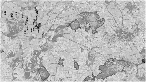
To examine the impact of different PCRs, 11 PCR levels (i.e. 80%, 85%, 90%, 95%, 99.5%, 99.6%, 99.7%, 99.73%, 99.8%, 99.9%, and 100%) are considered for each city, thus creating a set of 77 instances. The PCR faced by Geldmaat is equal to 99.73%, as already mentioned in Section 1. Each instance features a maximum route duration constraint equal to 480 min, which corresponds to a typical working day of eight hours. Real-road distances are taken into account. Citizens (identified by their permanent residence address) are considered to be covered if a replenished ATM exists within a specific (straight) distance r from their permanent residence address. This distance extends the five kilometre rule in the analysis of the DNB (see NFPS, 2017). It is determined by a function of the population density and number of available ATMs in a given geographical area and was provided by Geldmaat for our seven real-life instances. Figure 3 geographically represents an instance for Tilburg.

Figure 3. Tilburg instance with 35 ATMs (pinned locations) and the depot (drop).

5.1.1. Case study results

Table 3 presents the detailed computational results for the 77 real-life instances. Each row of this table reports the computational results of the TSMheu and MIP for one of the 77 test instances. The following information is indicated: the city (City), the PCR (PCR), the worst ($\mathsf{u}{\mathsf{b}}_{\mathsf{W}}$), average ($\mathsf{u}{\mathsf{b}}_{\mathsf{A}}$), and best (ub_B) upper bounds computed by the TSMheu along with the corresponding percentage gaps for the latter two (%${}_{\mathsf{ADB}},$ %${}_{\mathsf{BDB}}$) computed with respect to the best-known lower bound achieved by the MIP ($\mathsf{l}{\mathsf{b}}_{\mathsf{MIP}}$), the percentage gap between ub_B and the best computed upper bound ($\mathsf{u}{\mathsf{b}}_{\mathsf{MIP}}$) produced by the MIP (%${}_{\mathsf{BPB}}$); note here that negative gaps mean that the best solution found by the TSMheu is better than the best solution found by the MIP), and the average computation time of the TSMheu ($\mathsf{cp}{\mathsf{u}}_{\mathsf{Heu}}$) - all these values are averages over 10 runs. Additionally, we report the number of replenished ATMs (${\mathsf{S}}_{\mathsf{B}}$) along with the fill-rate indicating the percentage of replenished ATMs ($\mathsf{F}{\mathsf{R}}_{\mathsf{ATM}}$), and the number of vehicles required (${\mathsf{K}}_{\mathsf{R}}$) in the best solution found by the TSMheu (ub_B). Finally, we also report the percentage gap between the $\mathsf{u}{\mathsf{b}}_{\mathsf{MIP}}$ and $\mathsf{l}{\mathsf{b}}_{\mathsf{MIP}}$ (%${}_{\mathsf{MIP}}$) along with the computation time spent by the MIP ($\mathsf{cp}{\mathsf{u}}_{\mathsf{MIP}}$).

Table 3. Detailed computational results on the 77 real-life instances.

City	PCR (%)	$\mathsf{u}{\mathsf{b}}_{\mathsf{W}}$	$\mathsf{u}{\mathsf{b}}_{\mathsf{A}}$	%${}_{\mathsf{ADB}}$	ubB	%${}_{\mathsf{BDB}}$	%${}_{\mathsf{BPB}}$	SB	$\mathsf{F}{\mathsf{R}}_{\mathsf{ATM}}$	KR	$\mathsf{cp}{\mathsf{u}}_{\mathsf{Heu}}$	$\mathsf{u}{\mathsf{b}}_{\mathsf{MIP}}$	$\mathsf{l}{\mathsf{b}}_{\mathsf{MIP}}$	%${}_{\mathsf{MIP}}$	$\mathsf{cp}{\mathsf{u}}_{\mathsf{MIP}}$
	80	2531.2	2528.6	2.2	2524.8	2.0	–0.8	31	31.6	2	1306.4	2544.0	2473.6	2.8	TL
	85	2780.8	2776.0	2.2	2768.0	1.9	–0.1	34	34.7	2	1352.4	2771.2	2714.6	2.0	TL
	90	3267.2	3263.7	6.6	3257.6	6.4	–0.2	39	39.8	3	1261.9	3264.0	3048.3	6.6	TL
	95	3753.6	3750.7	4.5	3747.2	4.4	0.0	46	46.9	3	1354.2	3747.2	3584.0	4.4	TL
	99.5	5072.0	5068.8	4.7	5059.2	4.5	0.0	63	64.3	4	1318.3	5059.2	4832.3	4.5	TL
Amsterdam	99.6	5136.0	5134.4	4.1	5129.6	4.0	–	64	65.3	4	1317.0	–	4924.4	–	TL
	99.7	5273.6	5263.7	4.4	5254.4	4.3	0.2	66	67.3	4	1360.9	5241.6	5031.1	4.0	TL
	99.73	5331.2	5328.0	4.7	5321.6	4.5	–0.4	67	68.4	4	1429.3	5340.8	5080.2	4.9	TL
	99.8	5408.0	5404.8	3.6	5385.6	3.3	0.4	68	69.4	4	1429.0	5366.4	5207.9	3.0	TL
	99.9	5680.0	5667.5	3.8	5648.0	3.5	0.0	72	73.5	4	1444.7	5648.0	5452.4	3.5	TL
	100	6064.0	6059.8	4.6	6044.8	4.3	–	76	77.6	4	1705.8	–	5782.4	–	TL
	80	2332.8	2332.8	12.6	2332.8	12.6	–0.7	18	26.5	2	328.64	2348.8	2040.1	13.1	TL
	85	2656.0	2641.6	9.8	2636.8	9.6	–2.7	22	32.4	2	344.3	2710.4	2383.9	12.1	TL
	90	3379.2	3095.4	8.3	3056.0	7.1	–9.1	27	39.7	2	362.2	3360.0	2839.1	15.5	TL
	95	3875.2	3867.5	10.9	3859.2	10.7	–0.5	33	48.5	3	422.1	3878.4	3446.5	11.1	TL
	99.5	4428.8	4418.2	5.2	4406.4	5.0	–0.2	39	57.4	3	366.9	4412.8	4186.6	5.1	TL
Venlo	99.6	4480.0	4468.5	4.6	4451.2	4.2	0.1	40	58.8	3	416.5	4444.8	4262.8	4.1	TL
	99.7	4492.8	4482.9	6.7	4473.6	6.5	–0.1	40	58.8	3	385.6	4480.0	4180.8	6.7	TL
	99.73	4560.0	4544.6	7.9	4531.2	7.7	–7.3	41	60.3	3	451.6	4889.6	4184.5	14.4	TL
	99.8	4569.6	4550.7	6.7	4531.2	6.3	–0.1	41	60.3	3	441.9	4534.4	4246.7	6.3	TL
	99.9	4960.0	4957.8	11.1	4947.2	10.9	–0.4	42	61.8	4	420.6	4966.4	4409.5	11.2	TL
	100	5414.4	5401.6	9.6	5379.2	9.3	–0.1	47	69.1	4	457.6	5382.4	4881.3	9.3	TL
	80	1238.4	1239.7	0.1	1238.4	0.0	0.0	9	18.0	1	376.6	1238.4	1238.4	0.0	505.5
	85	1420.8	1420.8	0.0	1420.8	0.0	0.0	11	22.0	1	221.9	1420.8	1420.8	0.0	1468.1
	90	1929.6	1927.4	11.4	1926.4	11.4	–0.3	14	28.0	2	274.2	1932.8	1707.4	11.7	TL
	95	2284.8	2282.6	12.2	2281.6	12.2	0.0	17	34.0	2	357.9	2281.6	2003.9	12.2	TL
	99.5	2771.2	2771.2	2.0	2771.2	2.0	–0.2	23	46.0	2	285.9	2777.6	2715.4	2.2	TL
Almelo	99.6	2771.2	2771.2	0.7	2771.2	0.7	–0.2	23	46.0	2	278.2	2777.6	2753.1	0.9	TL
	99.7	2774.4	2774.4	0.0	2774.4	0.0	0.0	23	46.0	2	270.0	2774.4	2774.4	0.0	2193.4
	99.73	2780.8	2780.8	0.0	2780.8	0.0	0.0	23	46.0	2	258.0	2780.8	2780.8	0.0	2181.8
	99.8	2851.2	2847.0	0.1	2844.8	0.0	0.0	24	48.0	2	269.8	2844.8	2844.8	0.0	1344.0
	99.9	2979.2	2979.2	0.0	2979.2	0.0	0.0	26	52.0	2	186.4	2979.2	2979.2	0.0	2294.6
	100	3849.6	3849.3	8.3	3846.4	8.3	0.0	33	66.0	3	356.6	3846.4	3529.0	8.3	TL
	80	1411.2	1411.2	0.0	1411.2	0.0	0.0	15	42.9	1	100.0	1411.2	1411.2	0.0	45.0
	85	1488.0	1488.0	0.0	1488.0	0.0	0.0	16	45.7	1	80.3	1488.0	1488.0	0.0	16.5
	90	1952.0	1952.0	12.5	1952.0	12.5	0.0	18	51.4	2	90.0	1952.0	1708.5	12.5	TL
	95	2102.4	2102.4	0.0	2102.4	0.0	0.0	20	57.1	2	97.1	2102.4	2102.4	0.0	1220.3
	99.5	2515.2	2515.2	0.0	2515.2	0.0	0.0	26	74.3	2	110.3	2515.2	2515.2	0.0	206.4
Tilburg	99.6	2515.2	2515.2	0.0	2515.2	0.0	0.0	26	74.3	2	106.8	2515.2	2515.2	0.0	198.8
	99.7	2582.4	2582.4	0.0	2582.4	0.0	0.0	27	77.1	2	114.5	2582.4	2582.4	0.0	2302.6
	99.73	2582.4	2582.4	0.0	2582.4	0.0	0.0	27	77.1	2	113.5	2582.4	2582.4	0.0	2882.7
	99.8	2649.6	2646.7	0.0	2646.4	0.0	0.0	28	80.0	2	118.8	2646.4	2646.4	0.0	316.1
	99.9	2716.8	2715.8	0.1	2713.6	0.0	0.0	29	82.9	2	119.3	2713.6	2713.6	0.0	983.8
	100	2716.8	2716.5	0.1	2713.6	0.0	0.0	29	82.9	2	116.7	2713.6	2713.6	0.0	1358.7
	80	908.8	908.8	0.0	908.8	0.0	0.0	10	32.3	1	65.4	908.8	908.8	0.0	43.3
	85	982.4	982.4	0.0	982.4	0.0	0.0	11	35.5	1	114.0	982.4	982.4	0.0	20.7
	90	1078.4	1078.4	0.0	1078.4	0.0	0.0	12	38.7	1	110.1	1078.4	1078.4	0.0	14.9
	95	1222.4	1222.4	0.0	1222.4	0.0	0.0	14	45.2	1	96.5	1222.4	1222.4	0.0	17.98
	99.5	1689.6	1686.1	0.2	1683.2	0.0	0.0	19	61.3	2	81.9	1683.2	1683.2	0.0	1020.1
Arnhem	99.6	1712.0	1709.4	0.0	1708.8	0.0	0.0	19	61.3	2	82.2	1708.8	1708.8	0.0	430.0
	99.7	1760.0	1758.1	0.1	1756.8	0.0	0.0	20	64.5	2	86.0	1756.8	1756.8	0.0	452.2
	99.73	1772.8	1769.6	0.2	1766.4	0.0	0.0	20	64.5	2	85.6	1766.4	1766.4	0.0	322.0
	99.8	1772.8	1771.2	0.1	1769.6	0.0	0.0	20	64.5	2	82.6	1769.6	1769.6	0.0	133.1
	99.9	1852.8	1851.8	0.1	1849.6	0.0	0.0	21	67.7	2	87.4	1849.6	1849.6	0.0	198.7
	100	2051.2	2051.2	0.0	2051.2	0.0	0.0	24	77.4	2	95.9	2051.2	2051.2	0.0	29.6
	80	1280.0	1276.5	0.7	1267.2	0.0	0.0	13	40.6	1	44.2	1267.2	1267.2	0.0	2.3
	85	1408.0	1405.1	0.0	1404.8	0.0	0.0	15	46.9	1	59.1	1404.8	1404.8	0.0	57.9
	90	1513.6	1510.7	0.0	1510.4	0.0	0.0	16	50.0	1	48.1	1510.4	1510.4	0.0	21.0
	95	1942.4	1940.5	0.1	1939.2	0.0	0.0	19	59.4	2	70.1	1939.2	1939.2	0.0	2060.0
	99.5	2236.8	2233.0	0.3	2227.2	0.0	0.0	23	71.9	2	77.0	2227.2	2227.2	0.0	88.2
Almere	99.6	2300.8	2299.5	0.1	2297.6	0.0	0.0	24	75.0	2	89.4	2297.6	2297.6	0.0	613.6
	99.7	2300.8	2300.2	0.1	2297.6	0.0	0.0	24	75.0	2	84.0	2297.6	2297.6	0.0	137.7
	99.73	2300.8	2300.2	0.1	2297.6	0.0	0.0	24	75.0	2	84.8	2297.6	2297.6	0.0	525.7
	99.8	2307.2	2302.4	0.2	2297.6	0.0	0.0	24	75.0	2	82.3	2297.6	2297.6	0.0	128.0
	99.9	2371.2	2369.6	0.1	2368.0	0.0	0.0	25	78.1	2	88.9	2368.0	2368.0	0.0	220.4
	100	2374.4	2370.9	0.1	2368.0	0.0	0.0	25	78.1	2	86.1	2368.0	2368.0	0.0	163.7
	80	918.4	918.4	0.0	918.4	0.0	0.0	8	33.3	1	41.5	918.4	918.4	0.0	5.8
	85	1008.0	1002.9	1.7	985.6	0.0	0.0	9	37.5	1	43.8	985.6	985.6	0.0	4.0
	90	1068.8	1062.7	1.0	1052.8	0.0	0.0	10	41.7	1	25.5	1052.8	1052.8	0.0	3.1
	95	1216.0	1213.4	0.1	1212.8	0.0	0.0	12	50.0	1	25.3	1212.8	1212.8	0.0	5.6
	99.5	1516.8	1516.8	0.0	1516.8	0.0	0.0	16	66.7	1	38.9	1516.8	1516.8	0.0	1.1
Gouda	99.6	1516.8	1516.8	0.0	1516.8	0.0	0.0	16	66.7	1	38.2	1516.8	1516.8	0.0	0.8
	99.7	1516.8	1516.8	0.0	1516.8	0.0	0.0	16	66.7	1	38.0	1516.8	1516.8	0.0	0.8
	99.73	1516.8	1516.8	0.0	1516.8	0.0	0.0	16	66.7	1	37.8	1516.8	1516.8	0.0	0.4
	99.8	1516.8	1516.8	0.0	1516.8	0.0	0.0	16	66.7	1	37.8	1516.8	1516.8	0.0	0.4
	99.9	1779.2	1779.2	0.0	1779.2	0.0	0.0	17	70.8	1	40.3	1779.2	1779.2	0.0	13.2
	100	1862.4	1859.5	0.0	1859.2	0.0	0.0	18	75.0	2	43.9	1859.2	1859.2	0.0	12.8
Avg				2.4		2.3	–0.3				340.2			2.5	1650.2
Opt						49/77								49/77

Both methods were able to find optimal solutions for 49 out of the 77 instances with up to 50 ATMs. The corresponding average gaps (%${}_{\mathsf{BDB}},$ %${}_{\mathsf{MIP}}$) are equal to 2.3% and 2.5%, respectively. Additionally, TSMheu was able to find 25 better solutions than the MIP for the remaining 28 instances for which there is no provable optimality. Moreover, the highest fill rate ($\mathsf{F}{\mathsf{R}}_{\mathsf{ATM}}$) over all instances is only 82.9%, so a significant percentage of ATMs can potentially be closed even if the entire population has to be covered.

Table 4 reports the cost differences of the replenishment operations for each of the seven cities, between the current PCR Geldmaat is required to meet (i.e. 99.73%) and the other ten PCRs considered. We observe that small differences in the PCRs (e.g. 0.03% or 0.07%) affect the costs significantly. The impact differs across cities because of the differences in the dispersion of the population and ATM locations. Another important observation is that applying ATM replenishment strategies that deviate significantly from the required population coverage of 99.73% may result in either i) significantly higher total replenishment costs or ii) a violated PCR accompanied by only minor financial benefits. Replenishing ATMs that cover more than 99.73% of the population may result in higher total costs of 0.85% for a PCR equal to 99.8% and 7.15% for a PCR equal to 99.9%. On the contrary, replenishing ATMs covering less than 99.73% of the population results in reduced costs with 0.74% less for a PCR equal to 99.7%, 1.98% less for a PCR equal to 99.6%, and 2.97% less for a PCR equal to 99.5%. Thus, replenishment strategies such as the one introduced in this paper can be beneficial since they help fulfil the required PCR in a cost-efficient way. To illustrate this point, consider the seven cities representing 5.86% of the population of the Netherlands for 250 working days per year; a non-accurate replenishment strategy always covering 99.9% of the population may result in an unnecessary additional annual cost of 371,742.8 €.

Table 4. Impact of the PCR on the total cost for the seven cities of our study.

City	80%	85%	90%	95%	99.5%	99.6%	99.7%	99.73%	99.8%	99.9%	100%
Amsterdam	–52.48%	–47.99%	–38.79%	–29.59%	–4.93%	–3.61%	–1.50%	5,321.6 €	+0.84%	+6.13%	+13.59%
Venlo	–48.52%	–41.81%	–32.56%	–14.83%	–2.75%	–1.91%	–1.27%	4,531.2 €	+0.00%	+9.18%	+18.71%
Almelo	–55.47%	–48.91%	–30.72%	–17.95%	–0.35%	–0.35%	–0.23%	2,780.8 €	+2.30%	+7.13%	+38.32%
Tilburg	–45.35%	–42.38%	–24.41%	–18.59%	–2.60%	–2.60%	–0.00%	2,582.4 €	+2.48%	+5.08%	+5.08%
Arnhem	–48.55%	–44.38%	–38.95%	–30.80%	–4.71%	–3.26%	–0.54%	1,766.4 €	+0.18%	+4.71%	+16.12%
Almere	–44.85%	–38.86%	–34.26%	–15.60%	–3.06%	–0.00%	–0.00%	2,297.6 €	+0.00%	+3.06%	+3.06%
Gouda	–39.45%	–35.02%	–30.59%	–20.04%	–0.00%	–0.00%	–0.00%	1,516.8 €	+0.00%	+17.30%	+22.57%
Average	–49.00%	–43.81%	–33.48%	–21.31%	–2.97%	–1.98%	–0.74%	2,971.0 €	+0.85%	+7.15%	+16.66%

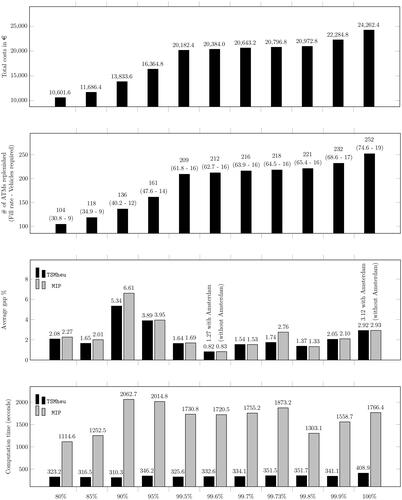
Figure 4 presents our aggregated computational findings for the seven major Dutch cities involving 1,003,519 citizens, 338 ATMs, and 19 cash distribution vehicles. Specifically, we show the impact of the PCR on 1) total replenishment costs, 2) the number of ATMs that need to be replenished along with the realised fill rate and number of cash distribution vehicles that need to be available for the related operations by considering the structure of the best solution found per instance, 3) the average gaps for the TSMheu and MIP, and 4) the average computation times for the TSMheu and the MIP. An interesting observation is that, on average, a PCR equal to 100% can be obtained by replenishing only 77.4% of the ATMs, while this fill rate is 64.5% for a PCR equal to 99.73%. Further, total replenishment costs, the total number of ATMs replenished, and the total number of vehicles required all rise when the PCR is set to 100%. Additional investment in distribution capacity is, however, only required if the required PCR is greater than 99.8%. On the computational side, both methods were able to compute high-quality solutions within reasonable (average) times of up to 408.9 s for the TSMheu and 2062.7 s for the MIP, especially given that the computed gaps may be overestimated, as not all the lower bounds provided by the MIP were proven to be optimal.

Figure 4. Aggregated results per PCR for seven major Dutch cities involving 1,003,519 citizens, 338 ATMs, and 19 cash distribution vehicles.

5.2. Synthetic instance generation

To further investigate the computational behaviour of the MIP and the tour-splitting metaheuristic TSMheu, we derived 144 new instances from nine instances of the distance-constrained capacitated vehicle routing problem (DCVRP) that can be found in Vigo (1999). Specifically, we made use of the DCVRP instances with at least 51 vertices, namely: D051-06c, D076-11c, D101-09c, D101-11c, D121-11c, D151-14b, D151-14c, D200-18b, and D200-18c. From these instances, we took the following information: (a) the total number of vertices, (b) the number of vehicles, (c) the maximum route duration, (d) the service time, (e) the Euclidean 2-dimensional coordinates of each vertex, and (f) the demand of each vertex. On the contrary, some new data had to be generated, namely the demand points that can be covered by the may-visit locations (or vertices) and a radius determining the coverage distance of each location. To create the new instances, we adopted the following process: first, the minimum distance between any two locations was calculated; the initial coverage radius r₀ was then set for all locations as the half of this distance. As a next step, the number of demand points for each location was set based on the demand of each location in the original DCVRP instance; the demand points were then randomly distributed around each location within a distance of r₀.

The previously described process allowed us to generate a set of nine instances with a coverage radius defined in such a way so that all demand points can be covered by exactly one location. In other words, all these nine instances have an overlap equal to 0%. For each instance, 16 more were generated by considering four distinct demand point coverage requirements (DPCR) equal to 85%, 90%, 95%, 100% of the total number of demand points and four distinct overlap levels equal to 0%, 10%, 30%, 50%. An instance with overlap equal to 0% has a total number of covered equal to the number of demand points. To generate instances with increasing overlaps, r₀ was gradually increased so that the total number of demand point coverings can get larger than the total number of demand points. For example, an instance with r₀ and a total number of n demand points has a total amount of $c_{r_0}^n$ coverings and 0% overlap. The same instance can generate another one with overlap 10% with a new service radius $r\prime >r_0$ if the total amount of coverings $c_{r_0}^n+c_{r\prime }^n-c_{r_0}^n/c_{r_0}^n$ is equal to 1.1. Note that attempting to solve an instance with DPCR equal to 100% and an overlap equal to 0% is equivalent to solving a DCVRP instance without capacity constraints. Similarly, attempting to solve an instance with DPCR equal to 100% is equivalent to solving an m-CTP instance with may-visit locations. The Euclidean two-dimensional distances between the locations of the synthetic instances have been rounded up to the closest integer.

5.2.1. Results on the synthetic instances

Figures 5 and 6 report on the computational behaviour of the TSMheu and MIP for a total set of 144 synthetic instances. A detailed presentation of this computational study can be found in A.

Figure 5. Aggregated computational results of the TSMheu and MIP with respect to different overlap levels.

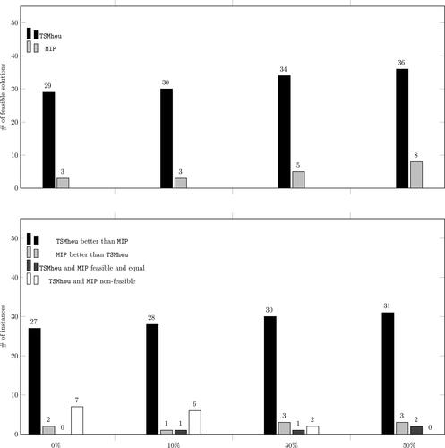
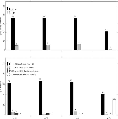
Figure 6. Aggregated computational results of the TSMheu and MIP with respect to different DPCR levels.

Figure 5 highlights the impact of the overlap levels on the effectiveness on the solution approaches. For each group of 36 instances with the same overlap, the top part of Figure 5 reports the number of feasible solutions found by the two methods, while the bottom part provides more details on which method achieves better solutions. Our main observation here is that when the overlap level gets higher, both solution methods appear to find more feasible solutions. We also observe that, overall, the TSMheu manages to find more feasible solutions. This is expected as higher overlap levels may create space to alternative solution structures that would not be possible otherwise. The quality of these solutions, however, could not be proved to be optimal as the MIP did not manage to close the optimality gap for any of the instances due to their large size. Last, both methods did not manage to find a feasible solution for 15 out of the 144 instances. Notice that for these instances a feasible may not exist due to the way we calculated the distances between the locations.

Figure 6 highlights the impact of the DPCR levels on the effectiveness of both solution approaches. For each group of 36 instances with the same DPCR, the top part of Figure 6 reports the number of feasible solutions found by the two methods, while the bottom part provides more details on which method achieves better solutions. Contrary to our observations regarding overlap levels, the main observation here is that when the DPCR level gets higher, both solution methods appear to find less feasible solutions. This can be explained by the fact that higher DPCR levels reduce the space of feasible solutions. The overall performance of the TSMheu appears to be better than the one of the MIP but again, no solutions could be proved to be optimal. Both methods did not manage to find a feasible solution for 15 out of the 144 instances. Notice again that for these instances a feasible may not exist due to the way we calculated the distances between the locations.

6. Conclusions

Cash payments are the dominant payment instrument in a large majority of sectors throughout Europe. In recent years, however, digital or contactless payments have become widely available (Esselink & Hernández, 2017). This trend has caused a gradual removal of ATMs in many European countries (de Groen et al., 2018). Inspired by the real-life case of ATM cash replenishment, we introduced and studied a new covering tour problem, namely, the VTPMCR that extends the literature by capturing the case in which only a proportion of demand needs to be covered. A compact formulation accompanied by a family of valid inequalities for efficiently solving small and medium-sized instances and a tour-splitting metaheuristic accompanied by local neighbourhood search are proposed. A computational study on 77 real-life instances showed the effectiveness of our compact formulation and of the metaheuristic for solving small and medium-sized real-life instances with up to 50 ATMs and 163,029 citizens to provable optimality. Specifically, we manage to solve 49 out of the 77 instances to optimality, with an average gap below 2.5% for both solution methods. We show that significant cost differences may occur when ATM replenishment strategies deviate from the required population coverage. Additionally, the impact of varying the minimum coverage requirements on replenishment costs and network utilisation is illustrated for seven major Dutch cities involving 1,003,519 citizens, 338 ATMs, and 19 cash distribution vehicles. Finally, to evaluate the competitiveness of both solution methods, 144 new synthetic instances are derived from a well-known set of benchmark instances. Our computational results showed that the behaviour of our metaheuristic solution approach is overall better than the one of our exact approach. Also, the problem’s parameter setting can affect the quality of the solutions obtained for both methods. Specifically, increased overlap levels and decreased coverage requirement levels seem to make the problem structure easier.

Acknowledgements

We would like to thank Geldmaat for providing real-life instances of banknote distribution. The views presented in the article are the sole responsibility of the authors.

Disclosure statement

No potential conflict of interest was reported by the authors.

Correction Statement

This article has been republished with minor changes. These changes do not impact the academic content of the article.

Additional information

Funding

The support by the Dutch Science Foundation [grant number 407-13-050] is gratefully acknowledged.

Notes

1 Geldmaat is a joint venture of the three largest banks of the Netherlands (i.e. ABN AMRO, ING, and Rabobank) responsible for providing logistical services such as cash collection, counting, and distribution.

Appendix.

Detailed computational results for the synthetic instances

Tables A.1–A.9 report on the computational behaviour of the TSMheu and MIP on a total set of 144 synthetic instances. Each of the nine tables reports the computational results for 16 instances produced by the same original instance, as described in Section 5.2. For each instance, the following information is provided: the DPCR, the worst ($\mathsf{u}{\mathsf{b}}_{\mathsf{W}}$), average ($\mathsf{u}{\mathsf{b}}_{\mathsf{A}}$), and best (ub_B) upper bounds computed by the TSMheu along with the corresponding percentage gaps for the latter two (%${}_{\mathsf{ADB}},$ %${}_{\mathsf{BPB}}$) computed with respect to the best-known lower bound achieved by the MIP ($\mathsf{l}{\mathsf{b}}_{\mathsf{MIP}}$), the percentage gap between ub_B and the best computed upper bound ($\mathsf{u}{\mathsf{b}}_{\mathsf{MIP}}$) produced by the MIP (%${}_{\mathsf{BPB}}$); note here that negative gaps mean that the best solution found by the TSMheu is better than the best solution found by the MIP), and the average computation time of the TSMheu ($\mathsf{cp}{\mathsf{u}}_{\mathsf{Heu}}$) – all these values are averages over 10 runs. When less than 10 runs produced a feasible solution, only ub_B is provided. Additionally, we report the number of visited locations (S_B) along with the fill-rate indicating the percentage of visited locations (FR), and the number of vehicles required (K_R) in the best solution found by the TSMheu (ub_B). Finally, we also report the percentage gap between the $\mathsf{u}{\mathsf{b}}_{\mathsf{MIP}}$ and $\mathsf{l}{\mathsf{b}}_{\mathsf{MIP}}$ (%MIP) along with the computation time spent by the MIP ($\mathsf{cp}{\mathsf{u}}_{\mathsf{MIP}}$).

Table A.1. Detailed computational results of the D051-06c family of instances.

Overlap (%)	DPCR (%)	$\mathsf{u}{\mathsf{b}}_{\mathsf{W}}$	$\mathsf{u}{\mathsf{b}}_{\mathsf{A}}$	%${}_{\mathsf{ADB}}$	ubB	%${}_{\mathsf{BDB}}$	%${}_{\mathsf{BPB}}$	SB	FR	KR	$\mathsf{cp}{\mathsf{u}}_{\mathsf{Heu}}$	$\mathsf{u}{\mathsf{b}}_{\mathsf{MIP}}$	$\mathsf{l}{\mathsf{b}}_{\mathsf{MIP}}$	%${}_{\mathsf{MIP}}$	$\mathsf{cp}{\mathsf{u}}_{\mathsf{MIP}}$
0	85	774	770.8	6.2	765	5.4	0.4	35	70.0	4	226.9	762	723.4	5.1	TL
10	85	757	752.9	4.5	751	4.3	0.0	33	66.0	4	217.3	751	719.1	4.3	TL
30	85	702	700.9	4.0	700	3.9	0.3	30	60.0	4	227.2	698	672.9	3.6	TL
50	85	636	636.0	3.3	636	3.3	0.0	27	54.0	4	215.5	636	614.8	3.3	TL
0	90	849	847.1	3.9	844	3.6	–0.2	39	78.0	5	254.2	846	814.0	3.8	TL
10	90	842	840.2	6.1	839	6.0	0.6	38	76.0	5	253.1	834	788.7	5.4	TL
30	90	793	781.8	3.4	776	2.7	0.0	35	70.0	4	252.5	776	754.9	2.7	TL
50	90	720	718.2	2.6	718	2.6	0.0	31	62.0	4	263.1	718	699.6	2.6	TL
0	95	953	948.9	4.8	942	4.1	0.5	44	88.0	5	299.3	937	903.6	3.6	TL
10	95	937	933.5	4.6	925	3.7	–0.5	43	86.0	5	281.6	930	890.4	4.3	TL
30	95	905	901.1	4.6	898	4.3	0.2	40	80.0	5	306.3	896	859.5	4.1	TL
50	95	850	848.6	5.3	847	5.1	0.2	37	74.0	5	308.6	845	804.0	4.9	TL
0	100	1137	1128.6	7.2	1122	6.7	–	50	100.0	6	337.2	–	1046.9	–	TL
10	100	1137	1128.6	7.2	1122	6.7	–	50	100.0	6	343.6	–	1046.9	–	TL
30	100	1137	1128.6	7.2	1122	6.7	–	50	100.0	6	349.9	–	1046.9	–	TL
50	100	1087	1084.3	6.7	1080	6.4	1.3	48	96.0	6	354.3	1066	1011.4	5.1	TL
Avg				5.1		4.7	0.2				280.7			4.0	TL
Opt						0/16								0/16

Table A.2. Detailed computational results of the D076-11c family of instances.

Overlap (%)	DPCR (%)	$\mathsf{u}{\mathsf{b}}_{\mathsf{W}}$	$\mathsf{u}{\mathsf{b}}_{\mathsf{A}}$	%${}_{\mathsf{ADB}}$	ubB	%${}_{\mathsf{BDB}}$	%${}_{\mathsf{BPB}}$	SB	FR	KR	$\mathsf{cp}{\mathsf{u}}_{\mathsf{Heu}}$	$\mathsf{u}{\mathsf{b}}_{\mathsf{MIP}}$	$\mathsf{l}{\mathsf{b}}_{\mathsf{MIP}}$	%${}_{\mathsf{MIP}}$	$\mathsf{cp}{\mathsf{u}}_{\mathsf{MIP}}$
0	85	1262	1255.1	12.0	1247	11.5	–	54	72.0	9	696.5	–	1104.0	–	TL
10	85	1209	1201.7	11.1	1198	10.8	–	51	68.0	8	631.0	–	1068.1	–	TL
30	85	1121	1112.1	11.7	1097	10.4	–	48	64.0	7	570.1	–	982.5	–	TL
50	85	1034	1027.1	9.6	1018	8.8	1.3	44	58.7	7	536.9	1005	928.3	7.6	TL
0	90	1392	1382.7	12.4	1361	11.0	–	59	78.7	9	731.9	–	1211.0	–	TL
10	90	1343	1337.3	11.6	1332	11.3	–	56	74.7	9	693.7	–	1181.7	–	TL
30	90	1234	1225.9	11.2	1219	10.7	–	51	68.0	8	637.0	–	1089.0	–	TL
50	90	1153	1148.5	11.5	1139	10.7	–	47	62.7	8	602.3	–	1016.8	–	TL
0	95	1570	1558.6	14.6	1537	13.4	–	65	86.7	10	750.0	–	1331.3	–	TL
10	95	1527	1518.9	13.9	1512	13.5	–	62	82.7	10	698.0	–	1307.6	–	TL
30	95	1402	1392.0	12.9	1383	12.3	–	56	74.7	9	615.5	–	1213.1	–	TL
50	95	1299	1294.4	12.1	1290	11.8	–	52	69.3	9	607.6	–	1138.1	–	TL
0	100	–	–	–	–	–	–	–	–	–	1235.8	–	1547.8	–	TL
10	100	–	–	–	–	–	–	–	–	–	1134.1	–	1527.6	–	TL
30	100	–	–	–	–	–	–	–	–	–	958.0	–	1482.0	–	TL
50	100	1608	1596.8	14.0	1583	13.3	–	64	85.3	11	764.0	–	1373.0	–	TL
Avg				12.2		11.5	1.3				741.4			7.6	TL
Opt						0/16								0/16

Table A.3. Detailed computational results of the D101-09c family of instances.

Overlap (%)	DPCR (%)	$\mathsf{u}{\mathsf{b}}_{\mathsf{W}}$	$\mathsf{u}{\mathsf{b}}_{\mathsf{A}}$	%${}_{\mathsf{ADB}}$	ubB	%${}_{\mathsf{BDB}}$	%${}_{\mathsf{BPB}}$	${\mathsf{S}}_{\mathsf{B}}$	FR	${\mathsf{K}}_{\mathsf{R}}$	$\mathsf{cp}{\mathsf{u}}_{\mathsf{Heu}}$	$\mathsf{u}{\mathsf{b}}_{\mathsf{MIP}}$	$\mathsf{l}{\mathsf{b}}_{\mathsf{MIP}}$	%${}_{\mathsf{MIP}}$	$\mathsf{cp}{\mathsf{u}}_{\mathsf{MIP}}$
0	85	1318	1306.0	7.9	1299	7.4	–	65	65.0	6	1006.9	–	1202.7	–	TL
10	85	1268	1258.1	7.4	1239	6.0	–	63	63.0	6	1001.4	–	1164.7	–	TL
30	85	1209	1202.7	8.2	1198	7.9	–	57	57.0	6	871.1	–	1103.6	–	TL
50	85	1154	1148.3	8.5	1141	7.9	–	55	55.0	6	878.4	–	1050.9	–	TL
0	90	1479	1471.9	9.2	1462	8.6	–	72	72.0	7	1183.7	–	1336.4	–	TL
10	90	1439	1430.7	9.5	1421	8.8	–	69	69.0	7	1072.5	–	1295.3	–	TL
30	90	1374	1369.4	9.3	1364	8.9	–	64	64.0	6	979.8	–	1242.0	–	TL
50	90	1307	1299.5	9.0	1286	8.0	–	61	61.0	6	1014.8	–	1182.7	–	TL
0	95	1682	1670.7	9.4	1663	9.0	–	82	82.0	8	1423.8	–	1513.4	–	TL
10	95	1631	1625.4	9.3	1618	8.9	–	79	79.0	8	1320.7	–	1474.5	–	TL
30	95	1580	1571.6	9.2	1551	8.0	–	74	74.0	7	1226.6	–	1427.0	–	TL
50	95	1496	1488.4	9.1	1479	8.5	–	70	70.0	7	1155.5	–	1353.0	–	TL
0	100	–	–	–	–	–	–	–	–	–	TLH	–	1846.3	–	TL
10	100	–	–	–	2019	10.8	–	97	97.0	9	TLH	–	1801.4	–	TL
30	100	1996	1977.2	11.5	1950	10.2	–	93	93.0	9	1685.8	–	1750.7	–	TL
50	100	1879	1866.9	10.5	1852	9.8	–	87	87.0	9	1431.3	–	1670.5	–	TL
Avg				9.1		8.6	–				1240.8			–	TL
Opt						0/16								0/16

Table A.4. Detailed computational results of the D101-11c family of instances.

Overlap (%)	DPCR (%)	$\mathsf{u}{\mathsf{b}}_{\mathsf{W}}$	$\mathsf{u}{\mathsf{b}}_{\mathsf{A}}$	%${}_{\mathsf{ADB}}$	ubB	%${}_{\mathsf{BDB}}$	%${}_{\mathsf{BPB}}$	SB	FR	KR	$\mathsf{cp}{\mathsf{u}}_{\mathsf{Heu}}$	$\mathsf{u}{\mathsf{b}}_{\mathsf{MIP}}$	$\mathsf{l}{\mathsf{b}}_{\mathsf{MIP}}$	%${}_{\mathsf{MIP}}$	$\mathsf{cp}{\mathsf{u}}_{\mathsf{MIP}}$
0	85	7282	7278.2	2.0	7272	1.9	–	73	73.0	8	TLH	–	7130.2	–	TL
10	85	6744	6733.6	2.0	6725	1.8	–	67	67.0	7	TLH	–	6601.1	–	TL
30	85	6054	6048.9	1.6	6040	1.5	–	60	60.0	7	1047.2	–	5950.1	–	TL
50	85	5281	5279.4	2.7	5278	2.7	–	52	52.0	6	783.7	–	5137.0	–	TL
0	90	8145	8139.4	1.8	8131	1.7	–	82	82.0	9	TLH	–	7992.8	–	TL
10	90	7680	7671.6	2.9	7663	2.8	–	77	77.0	8	TLH	–	7448.1	–	TL
30	90	6926	6921.1	1.7	6916	1.6	–0.3	69	69.0	7	1360.9	6940	6802.4	2.0	TL
50	90	6152	6148.0	2.5	6144	2.4	–0.2	61	61.0	7	1108.2	6155	5997.3	2.6	TL
0	95	9010	9001.9	1.6	8994	1.6	–	91	91.0	10	TLH	–	8853.4	–	TL
10	95	8551	8544.5	1.6	8533	1.5	–	86	86.0	9	TLH	–	8406.7	–	TL
30	95	7921	7908.9	2.0	7902	1.9	0.0	79	79.0	8	1468.0	7901	7754.0	1.9	TL
50	95	7045	7036.9	1.8	7031	1.8	–0.4	70	70.0	7	1190.5	7062	6907.0	2.2	TL
0	100	10006	9979.7	2.3	9952	2.0	–	100	100.0	11	TLH	–	9748.4	–	TL
10	100	9557	9542.5	1.7	9525	1.6	–	96	96.0	10	1775.3	–	9376.5	–	TL
30	100	9557	9542.5	1.7	9525	1.6	–	96	96.0	10	1789.8	–	9376.5	–	TL
50	100	9151	9141.6	1.5	9125	1.3	–	92	92.0	10	1710.4	–	9001.9	–	TL
Avg				2.0		1.9	–0.2				1552.1			2.2	TL
Opt						0/16								0/16

Table A.5. Detailed computational results of the D121-11c family of instances.

Overlap (%)	DPCR (%)	$\mathsf{u}{\mathsf{b}}_{\mathsf{W}}$	$\mathsf{u}{\mathsf{b}}_{\mathsf{A}}$	%${}_{\mathsf{ADB}}$	ubB	%${}_{\mathsf{BDB}}$	%${}_{\mathsf{BPB}}$	SB	FR	KR	$\mathsf{cp}{\mathsf{u}}_{\mathsf{Heu}}$	$\mathsf{u}{\mathsf{b}}_{\mathsf{MIP}}$	$\mathsf{l}{\mathsf{b}}_{\mathsf{MIP}}$	%${}_{\mathsf{MIP}}$	$\mathsf{cp}{\mathsf{u}}_{\mathsf{MIP}}$
0	85	5496	5456.7	8.4	5413	7.7	–	83	69.2	8	1754.5	–	4995.6	–	TL
10	85	5191	5178.9	8.6	5159	8.3	–	79	65.8	8	1654.3	–	4732.0	–	TL
30	85	4711	4698.4	8.5	4682	8.2	–	71	59.2	7	1486.4	–	4299.3	–	TL
50	85	4173	4159.1	6.9	4145	6.5	–	64	53.3	6	1401.2	–	3874.2	–	TL
0	90	6078	6042.0	8.4	6003	7.8	–	93	77.5	9	TLH	–	5532.2	–	TL
10	90	5759	5745.6	8.7	5729	8.4	–	87	72.5	9	TLH	–	5248.4	–	TL
30	90	5267	5246.8	8.6	5215	8.0	–	80	66.7	8	1737.5	–	4797.8	–	TL
50	90	4758	4746.5	8.5	4731	8.2	–	71	59.2	7	1518.9	–	4345.1	–	TL
0	95	6737	6723.0	8.5	6699	8.2	–	103	85.8	10	TLH	–	6149.4	–	TL
10	95	6471	6449.4	8.6	6423	8.2	–	98	81.7	10	TLH	–	5893.5	–	TL
30	95	5927	5917.5	8.5	5904	8.3	–	90	75.0	9	TLH	–	5414.1	–	TL
50	95	5467	5450.2	8.9	5438	8.7	–1.0	82	68.3	9	1671.3	5491	4967.0	9.5	TL
0	100	–	–	–	–	–	–	–	–	–	TLH	–	7109.8	–	TL
10	100	–	–	–	–	–	–	–	–	–	TLH	–	7054.2	–	TL
30	100	7030	7003.0	8.7	6949	8.0	–	106	88.3	10	TLH	–	6393.1	–	TL
50	100	6748	6731.2	8.6	6707	8.3	–	102	85.0	11	TLH	–	6150.7	–	TL
Avg				8.5		8.1	–1.0				1714.0			9.5	TL
Opt						0/16								0/16

Table A.6. Detailed computational results of the D151-14b family of instances.

Overlap (%)	DPCR (%)	$\mathsf{u}{\mathsf{b}}_{\mathsf{W}}$	$\mathsf{u}{\mathsf{b}}_{\mathsf{A}}$	%${}_{\mathsf{ADB}}$	ubB	%${}_{\mathsf{BDB}}$	%${}_{\mathsf{BPB}}$	SB	FR	KR	$\mathsf{cp}{\mathsf{u}}_{\mathsf{Heu}}$	$\mathsf{u}{\mathsf{b}}_{\mathsf{MIP}}$	$\mathsf{l}{\mathsf{b}}_{\mathsf{MIP}}$	%${}_{\mathsf{MIP}}$	$\mathsf{cp}{\mathsf{u}}_{\mathsf{MIP}}$
0	85	1932	1923.8	11.9	1917	11.6	–	98	65.3	10	TLH	–	1694.4	–	TL
10	85	1843	1833.4	11.1	1826	10.7	–	98	65.3	10	TLH	–	1630.1	–	TL
30	85	1701	1687.1	11.0	1678	10.5	–	84	56.0	9	TLH	–	1502.1	–	TL
50	85	1560	1546.8	10.6	1538	10.1	–	75	50.0	9	TLH	–	1383.4	–	TL
0	90	2146	2134.6	11.9	2119	11.3	–	109	72.7	11	TLH	–	1880.5	–	TL
10	90	2044	2033.0	11.5	2022	11.0	–	103	68.7	11	TLH	–	1799.6	–	TL
30	90	1895	1882.9	11.6	1869	10.9	–	95	63.3	10	TLH	–	1665.3	–	TL
50	90	1758	1748.6	11.5	1738	11.0	–	85	56.7	10	TLH	–	1547.6	–	TL
0	95	2422	2407.3	12.4	2398	12.0	–	123	82.0	14	TLH	–	2109.7	–	TL
10	95	2309	2296.7	12.3	2277	11.5	–	116	77.3	13	TLH	–	2015.1	–	TL
30	95	2126	2121.8	11.7	2109	11.2	–	106	70.7	12	TLH	–	1872.8	–	TL
50	95	1999	1989.9	11.4	1980	11.0	–	98	65.3	11	TLH	–	1762.5	–	TL
0	100	–	–	–	–	–	–	–	–	–	TLH	–	2527.7	–	TL
10	100	–	–	–	–	–	–	–	–	–	TLH	–	2448.8	–	TL
30	100	–	–	–	–	–	–	–	–	–	TLH	–	2323.2	–	TL
50	100	2539	2521.3	13.5	2490	12.4	–	123	82.0	14	TLH	–	2180.3	–	TL
Avg				11.7		11.2	–				TLH			–	TL
Opt						0/16								0/16

Table A.7. Detailed computational results of the D151-14c family of instances.

Overlap (%)	DPCR (%)	$\mathsf{u}{\mathsf{b}}_{\mathsf{W}}$	$\mathsf{u}{\mathsf{b}}_{\mathsf{A}}$	%${}_{\mathsf{ADB}}$	ubB	%${}_{\mathsf{BDB}}$	%${}_{\mathsf{BPB}}$	SB	FR	KR	$\mathsf{cp}{\mathsf{u}}_{\mathsf{Heu}}$	$\mathsf{u}{\mathsf{b}}_{\mathsf{MIP}}$	$\mathsf{l}{\mathsf{b}}_{\mathsf{MIP}}$	%${}_{\mathsf{MIP}}$	$\mathsf{cp}{\mathsf{u}}_{\mathsf{MIP}}$
0	85	1930	1918.8	11.8	1906	11.2	–	98	65.3	10	TLH	–	1692.3	–	TL
10	85	1836	1830.0	10.8	1814	10.1	–	97	64.7	10	TLH	–	1631.5	–	TL
30	85	1677	1670.1	10.8	1664	10.5	–	83	55.3	9	TLH	–	1489.3	–	TL
50	85	1560	1547.7	10.5	1536	9.8	–	78	52.0	8	TLH	–	1385.9	–	TL
0	90	2144	2133.2	12.0	2124	11.6	–	109	72.7	12	TLH	–	1877.3	–	TL
10	90	2050	2039.7	11.7	2031	11.4	–	103	68.7	11	TLH	–	1800.4	–	TL
30	90	1865	1854.2	11.2	1844	10.7	–	92	61.3	10	TLH	–	1646.2	–	TL
50	90	1755	1747.7	11.5	1735	10.9	–	86	57.3	9	TLH	–	1546.4	–	TL
0	95	2420	2405.6	12.2	2397	11.9	–	124	82.7	13	TLH	–	2112.3	–	TL
10	95	2316	2305.2	12.5	2292	12.0	–	116	77.3	13	TLH	–	2016.0	–	TL
30	95	2098	2088.2	12.1	2070	11.3	–	105	70.0	11	TLH	–	1835.4	–	TL
50	95	1998	1993.5	11.6	1989	11.4	–	98	65.3	11	TLH	–	1761.5	–	TL
0	100	–	–	–	–	–	–	–	–	–	TLH	–	2530.8	–	TL
10	100	–	–	–	–	–	–	–	–	–	TLH	–	2450.0	–	TL
30	100	2757	2706.0	15.6	2684	14.9	–	130	86.7	14	TLH	–	2283.8	–	TL
50	100	2573	2546.9	13.7	2530	13.1	–	124	82.7	14	TLH	–	2197.9	–	TL
Avg				12.0		11.5	–				TLH			–	TL
Opt						0/16								0/16

Table A.8. Detailed computational results of the D200-18b family of instances.

Overlap (%)	DPCR (%)	$\mathsf{u}{\mathsf{b}}_{\mathsf{W}}$	$\mathsf{u}{\mathsf{b}}_{\mathsf{A}}$	%${}_{\mathsf{ADB}}$	ubB	%${}_{\mathsf{BDB}}$	%${}_{\mathsf{BPB}}$	SB	FR	KR	$\mathsf{cp}{\mathsf{u}}_{\mathsf{Heu}}$	$\mathsf{u}{\mathsf{b}}_{\mathsf{MIP}}$	$\mathsf{l}{\mathsf{b}}_{\mathsf{MIP}}$	%${}_{\mathsf{MIP}}$	$\mathsf{cp}{\mathsf{u}}_{\mathsf{MIP}}$
0	85	2421	2412.4	13.3	2391	12.5	–	128	64.3	13	TLH	–	2092.7	–	TL
10	85	2341	2321.7	12.3	2289	11.1	–	122	61.3	12	TLH	–	2035.9	–	TL
30	85	2142	2134.8	12.5	2116	11.7	–	110	55.3	11	TLH	–	1868.5	–	TL
50	85	1912	1898.8	12.0	1885	11.4	–	99	49.7	10	TLH	–	1670.0	–	TL
0	90	2696	2686.3	12.8	2671	12.3	–	142	71.4	15	TLH	–	2342.3	–	TL
10	90	2608	2590.5	12.6	2564	11.7	–	135	67.8	14	TLH	–	2265.1	–	TL
30	90	2408	2394.7	13.1	2383	12.7	–	124	62.3	13	TLH	–	2079.8	–	TL
50	90	2163	2153.5	12.0	2139	11.4	–	110	55.3	12	TLH	–	1895.2	–	TL
0	95	3047	3025.6	13.2	3008	12.7	–	160	80.4	16	TLH	–	2626.4	–	TL
10	95	2954	2944.3	14.4	2923	13.8	–	153	76.9	15	TLH	–	2519.6	–	TL
30	95	2728	2716.9	13.3	2708	13.0	–	140	70.4	15	TLH	–	2355.7	–	TL
50	95	2464	2445.8	13.1	2432	12.6	–	126	63.3	13	TLH	–	2124.8	–	TL
0	100	–	–	–	–	–	–	–	–	–	TLH	–	3131.7	–	TL
10	100	–	–	–	–	–	–	–	–	–	TLH	–	3120.7	–	TL
30	100	3496	3454.9	17.2	3389	15.6	–	172	86.4	18	TLH	–	2860.0	–	TL
50	100	3256	3234.1	14.6	3203	13.8	–	163	81.9	18	TLH	–	2761.6	–	TL
Avg				13.3		12.6	–				TLH			–	TL
Opt						0/16								0/16

Table A.9. Detailed computational results of the D200-18c family of instances.

Overlap (%)	DPCR (%)	$\mathsf{u}{\mathsf{b}}_{\mathsf{W}}$	$\mathsf{u}{\mathsf{b}}_{\mathsf{A}}$	%${}_{\mathsf{ADB}}$	ubB	%${}_{\mathsf{BDB}}$	%${}_{\mathsf{BPB}}$	${\mathsf{S}}_{\mathsf{B}}$	FR	${\mathsf{K}}_{\mathsf{R}}$	$\mathsf{cp}{\mathsf{u}}_{\mathsf{Heu}}$	$\mathsf{u}{\mathsf{b}}_{\mathsf{MIP}}$	$\mathsf{l}{\mathsf{b}}_{\mathsf{MIP}}$	%${}_{\mathsf{MIP}}$	$\mathsf{cp}{\mathsf{u}}_{\mathsf{MIP}}$
0	85	2420	2407.7	12.9	2391	12.3	–	128	64.3	13	TLH	–	2097.1	–	TL
10	85	2329	2317.9	13.3	2309	13.0	–	121	60.8	12	TLH	–	2008.7	–	TL
30	85	2149	2138.8	12.6	2127	12.1	–	111	55.8	12	TLH	–	1869.5	–	TL
50	85	1889	1877.6	10.3	1867	9.8	–	99	49.7	10	TLH	–	1683.9	–	TL
0	90	2702	2690.0	13.5	2677	13.1	–	142	71.4	14	TLH	–	2327.3	–	TL
10	90	2591	2581.3	12.8	2569	12.4	–	139	69.8	14	TLH	–	2251.4	–	TL
30	90	2398	2392.9	12.7	2381	12.2	–	124	62.3	13	TLH	–	2090.1	–	TL
50	90	2151	2141.8	13.6	2135	13.3	–	109	54.8	12	TLH	–	1850.4	–	TL
0	95	3044	3030.5	13.3	3010	12.7	–	160	80.4	17	TLH	–	2627.0	–	TL
10	95	2926	2917.4	13.8	2906	13.4	–	152	76.4	16	TLH	–	2515.8	–	TL
30	95	2719	2707.7	13.2	2695	12.8	–	140	70.4	14	TLH	–	2350.0	–	TL
50	95	2442	2433.4	13.4	2413	12.6	–	124	62.3	13	TLH	–	2108.2	–	TL
0	100	–	–	–	–	–	–	–	–	–	TLH	–	3109.5	–	TL
10	100	–	–	–	–	–	–	–	–	–	TLH	–	3070.1	–	TL
30	100	3476	3439.4	16.2	3407	15.4	–	172	86.4	18	TLH	–	2882.3	–	TL
50	100	3167	3153.8	14.7	3133	14.1	–	160	80.4	17	TLH	–	2690.6	–	TL
Avg				13.3		12.8	–				TLH			–	TL
Opt						0/16								0/16

References

- Baldacci, R., Boschetti, M. A., Maniezzo, V., & Zamboni, M. (2005). Scatter search methods for the covering tour problem. In Metaheuristic optimization via memory and evolution (pp. 59–91). Springer.
- Bulhões, T., Hà, M. H., Martinelli, R., & Vidal, T. (2018). The vehicle routing problem with service level constraints. European Journal of Operational Research, 265(2), 544–558. https://doi.org/https://doi.org/10.1016/j.ejor.2017.08.027
- Clarke, G., & Wright, J. W. (1964). Scheduling of vehicles from a central depot to a number of delivery points. Operations Research, 12(4), 568–581. https://doi.org/https://doi.org/10.1287/opre.12.4.568
- de Groen, W. P., Kilhoffer, Z., & Musmeci, R. (2018). The future of EU ATM markets. Impacts of digitalisation and pricing policies on business models. CEPS Research Report, October 2018. Technical Report, Centre for European Policy Studies.
- DNBulletin. (2018). Cash or card? The customer decides. https://www.dnb.nl/en/news/news-and-archive/DNBulletin2018/dnb379982.jsp#.
- Escalona, P., Ordóñez, F., & Marianov, V. (2015). Joint location-inventory problem with differentiated service levels using critical level policy. Transportation Research Part E: Logistics and Transportation Review, 83, 141–157. https://doi.org/https://doi.org/10.1016/j.tre.2015.09.009
- Esselink, H., & Hernández, L. (2017). The use of cash by households in the euro area. Technical Report 201. European Central Bank.
- Flores-Garza, D. A., Salazar-Aguilar, M. A., Ngueveu, S. U., & Laporte, G. (2017). The multi-vehicle cumulative covering tour problem. Annals of Operations Research, 258(2), 761–780. https://doi.org/https://doi.org/10.1007/s10479-015-2062-7
- Gillett, B. E., & Miller, L. R. (1974). A heuristic algorithm for the vehicle-dispatch problem. Operations Research, 22(2), 340–349. https://doi.org/https://doi.org/10.1287/opre.22.2.340
- Ha, M. H., Bostel, N., Langevin, A., & Rousseau, L.-M. (2013). An exact algorithm and a metaheuristic for the multi-vehicle covering tour problem with a constraint on the number of vertices. European Journal of Operational Research, 226(2), 211–220. https://doi.org/https://doi.org/10.1016/j.ejor.2012.11.012
- Hachicha, M., Hodgson, M. J., Laporte, G., & Semet, F. (2000). Heuristics for the multi-vehicle covering tour problem. Computers & Operations Research, 27(1), 29–42. https://doi.org/https://doi.org/10.1016/S0305-0548(99)00006-4
- Hensher, D. A., & Houghton, E. (2004). Performance-based quality contracts for the bus sector: Delivering social and commercial value for money. Transportation Research Part B: Methodological, 38(2), 123–146. https://doi.org/https://doi.org/10.1016/S0191-2615(03)00004-3
- Hodgson, M. J., Laporte, G., & Semet, F. (1998). A covering tour model for planning mobile health care facilities in Suhum District, Ghama. Journal of Regional Science, 38(4), 621–638. https://doi.org/https://doi.org/10.1111/0022-4146.00113
- Ibarra-Rojas, O. J., Giesen, R., & Rios-Solis, Y. A. (2014). An integrated approach for timetabling and vehicle scheduling problems to analyze the trade-off between level of service and operating costs of transit networks. Transportation Research Part B: Methodological, 70, 35–46. https://doi.org/https://doi.org/10.1016/j.trb.2014.08.010
- Jonker, N., Hernandez, L., de Vree, R., & Zwaan, P. (2018). From cash to cards. How debit card payments overtook cash in the Netherlands. DNB Occasional Studies 1601. Central Bank, Research Department.
- Jozefowiez, N. (2014). A branch-and-price algorithm for the multivehicle covering tour problem. Networks, 64(3), 160–168. https://doi.org/https://doi.org/10.1002/net.21564
- Kammoun, M., Derbel, H., Ratli, M., & Jarboui, B. (2017). An integration of mixed vnd and vns: The case of the multivehicle covering tour problem. International Transactions in Operational Research, 24(3), 663–679. https://doi.org/https://doi.org/10.1111/itor.12355
- Karaoğlan, İ., Erdoğan, G., & Koç, Ç. (2018). The multi-vehicle probabilistic covering tour problem. European Journal of Operational Research, 271(1), 278–287. https://doi.org/https://doi.org/10.1016/j.ejor.2018.05.005
- Krauth, E., Moonen, H., Popova, V., & Schut, M. C. (2005). Performance measurement and control in logistics service providing. ICEIS 2005 - Proceedings of the 7th International Conference on Enterprise Information Systems. 239–247.
- Labbé, M., & Laporte, G. (1986). Maximizing user convenience and postal service efficiency in post box location. Belgian Journal of Operations Research, Statistics and Computer Science, 26, 21–35.
- Labbé, M., Laporte, G., Martín, I. R., & Gonzalez, J. J. S. (2004). The ring star problem: Polyhedral analysis and exact algorithm. Networks, 43(3), 177–189. https://doi.org/https://doi.org/10.1002/net.10114
- Lai, K-h. (2004). Service capability and performance of logistics service providers. Transportation Research Part E: Logistics and Transportation Review, 40(5), 385–399. https://doi.org/https://doi.org/10.1016/j.tre.2004.01.002
- Lin, J.-R., & Yang, T.-H. (2011). Strategic design of public bicycle sharing systems with service level constraints. Transportation Research Part E: logistics and Transportation Review, 47(2), 284–294. https://doi.org/https://doi.org/10.1016/j.tre.2010.09.004
- Lopes, R., Souza, V. A., & da Cunha, A. S. (2013). A branch-and-price algorithm for the multi-vehicle covering tour problem. Electronic Notes in Discrete Mathematics, 44, 61–66. https://doi.org/https://doi.org/10.1016/j.endm.2013.10.010
- Moons, K., Waeyenbergh, G., & Pintelon, L. (2019). Measuring the logistics performance of internal hospital supply chains–a literature study. Omega, 82, 205–217. https://doi.org/https://doi.org/10.1016/j.omega.2018.01.007
- Murakami, K. (2018). Iterative column generation algorithm for generalized multi-vehicle covering tour problem. Asia-Pacific Journal of Operational Research, 35(04), 1850021–1850022. https://doi.org/https://doi.org/10.1142/S0217595918500215
- Naji-Azimi, Z., Renaud, J., Ruiz, A., & Salari, M. (2012). A covering tour approach to the location of satellite distribution centers to supply humanitarian aid. European Journal of Operational Research, 222(3), 596–605. https://doi.org/https://doi.org/10.1016/j.ejor.2012.05.001
- NFPS. (2017). Interim report for 2017 on accessibility of ATMs and cash deposit facilities in the Netherlands. Technical Report, National Forum on the Payment System.
- Pham, T. A., Hà, M. H., & Nguyen, X. H. (2017). Solving the multi-vehicle multi-covering tour problem. Computers and Operations Research, 88, 258–278.
- Prins, C., Labadi, N., & Reghioui, M. (2009). Tour splitting algorithms for vehicle routing problems. International Journal of Production Research, 47(2), 507–535. https://doi.org/https://doi.org/10.1080/00207540802426599
- Prins, C., Lacomme, P., & Prodhon, C. (2014). Order-first split-second methods for vehicle routing problems: A review. Transportation Research Part C: Emerging Technologies, 40, 179–200. https://doi.org/https://doi.org/10.1016/j.trc.2014.01.011
- Sawik, T. (2015). On the fair optimization of cost and customer service level in a supply chain under disruption risks. Omega, 53, 58–66. https://doi.org/https://doi.org/10.1016/j.omega.2014.12.004
- Tricoire, F., Graf, A., & Gutjahr, W. J. (2012). The bi-objective stochastic covering tour problem. Computers & Operations Research, 39(7), 1582–1592. https://doi.org/https://doi.org/10.1016/j.cor.2011.09.009
- Vidal, T., Crainic, T. G., Gendreau, M., & Prins, C. (2014). A unified solution framework for multi-attribute vehicle routing problems. European Journal of Operational Research, 234(3), 658–673. https://doi.org/https://doi.org/10.1016/j.ejor.2013.09.045
- Vigo, D. (1999). VRPLIB: a vehicle routing problem library. http://www.or.deis.unibo.it/research/_pages/ORinstances/VRPLIB/VRPLIB.html.
- Zhang, Y., Feng, Z., Zhang, S., & Song, J. (2018). The effects of service level on bot transport project contract. Transportation Research Part E: Logistics and Transportation Review, 118, 184–206. https://doi.org/https://doi.org/10.1016/j.tre.2018.07.013