A heuristic approach for the distance-based critical node detection problem in complex networks

Abstract

The distance-based critical node problem involves identifying a subset of nodes in a network whose removal minimises a pre-defined distance-based connectivity measure. Having the classical critical node problem as a special case, the distance-based critical node problem is computationally challenging. In this article, we study the distance-based critical node problem from a heuristic algorithm perspective. We consider the distance-based connectivity objective whose goal is to minimise the number of node pairs connected by a path of length at most k, subject to budgetary constraints. We propose a centrality based heuristic which combines a backbone-based crossover procedure to generate good offspring solutions and a centrality-based neighbourhood search to improve the solution. Extensive computational experiments on real-world and synthetic graphs show the effectiveness of the developed heuristic in generating good solutions when compared to exact solution. Our empirical results also provide useful insights for future algorithm development.

Keywords:

• Distance-based critical node problem
• hop distance
• heuristics
• centrality
• breadth first search

1. Introduction

Assessment of system vulnerability to adversarial attacks has become an important concern to organisations especially in the wake of security threats around the world. Moreover, natural hazards such as environmental disasters and disease epidemics in recent times have led to large scale disruptions in social and economic activities. Although it could be rather impossible to avoid some of these occurrences, it is indeed necessary to curtail their impact on system performance. A strategic way of doing this is to identify elements of a system that are critical in maintaining optimum system performance in order to protect them. In other words, we are identifying the parts of a system whose failure would result in a breakdown of the system. The notion of performance in a network connotes different meaning depending on the topology of the system and the application being considered. For instance, in transportation networks, performance is reflected in the speed of commute of passengers, goods, and services from an origin point to a destination point. In communication networks, efficiency in communication is key since certain crucial information need to be transmitted within a specific time space or to as many individuals or groups of individuals as possible. The associated problem as studied in the optimisation community is termed critical node detection problem (CNP), as introduced in Arulselvan et al. (2009). Given an undirected graph $G=(V,E)$ with $n=\left|V\right|$ nodes (vertices) and $m=\left|E\right|,$ the problem (CNP) is to identify a subset of nodes of limited cardinality, whose deletion results in a subgraph of maximum disconnectivity with respect to a predefined connectivity metric.

CNP finds interesting applications in various fields such as telecommunication networks (Arulselvan et al., 2007), studies on biological molecules and drug design (Boginski & Commander, 2009), epidemiology (Arulselvan et al., 2007; Nandi & Medal, 2016), emergency response, and transportation engineering (Matisziw & Murray, 2009). In social network analysis, the concept of key players relates to the idea of critical nodes where members of a social network that are influential for diffusion of information or rumours are targeted (Borgatti, 2006). This is of practical benefit in a public health context where crucial health information is to be disseminated across communities as well as to stop the widespread of malicious news. Similarly, in security and defence operations, “neutralising” certain individuals in a terrorist network ensures disruption of communication within such a network, eventually limiting the possibility of the launch of a large scale attack (Arulselvan et al., 2007).

Studies on the critical node problem can be grouped into two broad categories, namely fragmentation-based connectivity objective and distance-based connectivity objective. Within fragmentation-based CNP, popular connectivity metrics are to:

• minimise the total number of connected node pairs in the resultant subgraph (e.g. Addis et al., 2013; Aringhieri et al., 2016b; Arulselvan et al., 2009; Di Summa et al., 2012; Purevsuren et al., 2016; Ventresca, 2012; Ventresca & Aleman, 2015; Veremyev et al., 2014; Zhou et al., 2018)

• maximise the total number of connected components in the residual graph (e.g. Aringhieri et al., 2016a; Shen & Smith, 2012; Veremyev et al., 2014)

• minimise the size of the largest connected component in the residual graph (e.g. Aringhieri et al., 2016a; Shen & Smith, 2012; Shen et al., 2012)

Other variants of the fragmentation-based CNP studied in literature include the cardinality-constrained critical node problem (Arulselvan et al., 2011) and the component-cardinality-constrained critical node problem (Lalou & Kheddouci, 2019; Lalou et al., 2016). Bi-objective variants of the CNP have also been considered. Ventresca et al. (2018) considered a bi-objective CNP that maximises the number of connected components while minimising the variance of the sizes of the components. Recently, Li et al. (2019) studied a bi-objective variant that simultaneously minimises pairwise connectivity of the induced graph and the cost of removing the critical nodes. This latter bi-objective variant is important when the budget on the critical node set is not known a priori thus allowing the decision maker to optimise the connectivity objective as well as the cost of deleting the critical node set. A similar multi-objective problem that is based on a cascade model was studied in Zhang et al. (2020). The stochastic and robust versions of the critical node problem have also been studied (e.g. Hosteins & Scatamacchia, 2020; Naoum-Sawaya & Buchheim, 2016). It is worth noting that the aforementioned studies on the fragmentation-based CNP are restricted to individual node removals and hence do not consider the structural relationships of the critical node set. Walteros et al. (2019) studied a generalisation of the CNP to the so-called critical node structure detection problem where the set of nodes to be deleted form a specific structure, Thus, the problem becomes further constrained by the desired structure of the critical node set such as cliques and stars giving rise to the new terms critical cliques and critical stars.

The second category of the CNP, hereafter referred to as distance-based critical node problem (DCNP) which is the focus of our study, incorporates a distance metric in its connectivity objective. Unlike fragmentation-based CNP, the DCNP does not only consider whether a pair of nodes is connected but also seeks to measure the extent of connectivity between them. This is particularly important in communication and social network contexts, where disconnection cannot be limited to absence of a path between node pairs. In such contexts, if nodes are separated by distances long enough, they can be seen as practically disconnected (Borgatti, 2006; Veremyev et al., 2014). The importance of distance-based measures was reiterated in a study on network robustness from an information theory perspective (Schieber et al., 2016). The authors observed that certain structural deviations from the input network are left undetected by traditional CNP metrics.

Traditional exact algorithms such as branch-and-bound and branch-and-cut have been employed to solve critical node detection problem (e.g. Arulselvan et al., 2009; Di Summa et al., 2012; Veremyev et al., 2014). However, due to its combinatorial nature, the complexity of the CNP grows significantly with the size of the network. As a result, the CNP has only been solved exactly on medium sparse network instances up to an instance with 1612 nodes and 2106 edges in reasonable computational time (see Veremyev et al., 2014, p. 1257). To mitigate this gap, heuristic algorithms have been developed to provide good solution to larger instances of the CNP. For example, Ventresca and Aleman (2015) proposed a greedy heuristic algorithm that is based on a modified depth first search. Two new neighbourhoods were developed by Aringhieri et al. (2016b) and used within a variable neighbourhood search solution framework. The new neighbourhoods are more computationally efficient than the traditional two node exchange. Aringhieri et al. (2016a) proposed a genetic algorithm for the classic CNP as well as its cardinality-constrained variant. A Greedy Randomised Adaptive Search Procedure (GRASP) with Path Relinking (PR) mechanism was proposed for the classic CNP by Purevsuren et al. (2016). Recently, Zhou et al. (2018) developed a memetic algorithm for both classic and cardinality-constrained variants of CNP. For a detailed discussion on heuristic solution methods as well as current developments in their application to combinatorial optimisation problems, we refer the reader to Silver (2004) as well as Aickelin and Clark (2011). To the best of our knowledge, the memetic algorithm proposed by Zhou et al. (2018) is the current state-of-the-art heuristic algorithm for the traditional critical node problem based on computational experiments on 26 real-world and 16 synthetic benchmark instances. Memetic algorithm has seen successful applications as a solution method to network problems related to the critical node detection problem as well as other $\mathcal{N}\mathcal{P}$-hard problems (e.g. Wang et al., 2020; Yadegari et al., 2019)

Unlike the fragmentation-based critical node problem, research studies on the distance-based critical node problem are quite limited in number. The only computational studies on the DCNP are those by Veremyev et al. (2015) and much recently by Hooshmand et al. (2020) and Alozie et al. (2021) all of which follow traditional exact route hence were limited to small to medium graph sizes. The remaining two studies on the DCNP are those of Aringhieri et al. (2016c, 2019). The first was a preliminary analysis of the DCNP with some suggestions on design of heuristic algorithms. In the latter, the authors analysed the complexity of some classes of the DCNP, then proposed polynomial and pseudo-polynomial algorithms for those classes of the DCNP on graphs with special structure such as trees and paths. However, no computational results was presented in either of their studies.

To the best of our knowledge, our study is the first to address the distance-based critical node problem from a heuristic perspective. We demonstrate the efficiency of our proposed algorithm in comparison to the current state-of-the-art algorithm on both real-world and synthetic graphs.

1.1. Contributions

Our main contributions consist of the following:

1. We describe a new heuristic algorithm for the distance-based critical node problem. The feasible solution construction procedure utilizes centrality measures along with the idea of backbone-based crossovers to construct good feasible solutions. The neighbourhood search procedure uses a newly developed two-stage node exchange strategy to focus local search on a reduced centrality-based neighborhood, thus, making the search more efficient.

2. The proposed algorithm yields competitive results on both real-world and synthetic graphs. In particular for the real world instances, our heuristic algorithm matches the exact optimal solutions for all 28 instances. For the synthetic graphs which comprise of 54 instances, the heuristic achieves the optimal objective value or best known upper bounds on 10 of the instances and discovers new upper bounds on 33 of the instances within very short time duration in comparison to the exact algorithm.

3. Our empirical results provide useful insights to the effect of topological structures of certain model networks on algorithm behaviour.

1.2. Organisation

The rest of the article is structured as follows. In Section 2, we recapitulate the description of distance-based critical node problem with definitions of distance connectivity measures. Section 3 describes the proposed heuristic algorithm in detail. In Section 4, parameter settings and results of our computational experiments are presented. For real-world and synthetic network instances, we compare the performance of our proposed heuristic algorithm with results of exact algorithms. We conclude the article with some future work in Section 5.

2. Problem description

Given an input graph $G=(V,E)$ with $n=\left|V\right|$ nodes (vertices) and $m=|E\subseteq V\times V|$ edges, as well as a positive integer B, the distance-based critical node problem aims to find a subset of nodes of cardinality at most B, whose removal minimises a certain distance-based connectivity objective. Different distance-based connectivity functions were defined by Veremyev et al. (2015), however, computational studies have focused on three main distance-based connectivity measures:

• Minimise the total number of pairs of nodes connected by a hop distance of at most k (Alozie et al., 2021; Veremyev et al., 2015).

• Minimise Harary index or efficiency (Alozie et al., 2021; Veremyev et al., 2015).

• Minimise Weiner index or characteristic path length (Hooshmand et al., 2020).

In this study, we focus on the first distance-based connectivity objective which is the most studied and which has interesting real life applications, for example in transportation engineering. The distance function is defined by: (1) $$f(d)=\{\begin{array}{cc}1,\hfill & \hspace{1em}\text{if}\mathrm{ }d\le k\hfill \\ 0,\hfill & \hspace{1em}\text{if}\mathrm{ }d>k\hfill \end{array}$$(1) where d is the distance (shortest path length) between node pairs in the induced subgraph $G^S=G[V\setminus S],$ and k is a given positive integer representing the cut-off hop distance. The special case where $k\ge n-1$ is the traditional CNP version which minimises the number of connected node pairs in the residual graph. Interesting instances for this class are graphs with a small diameter, and thus, a large proportion of nodes connected within a small number of hops. We refer to this proportion as the initial percentage k-distance connectivity (% k-Conn).

3. Heuristic for distance-based critical node problem

This section describes the proposed heuristic algorithm for the distance-based critical node problem. The underlying idea of the proposed heuristic framework is akin to the memetic algorithm recently proposed for the classical critical node problem (Zhou et al., 2018), however, with some striking differences as described later in the article (Subsection 3.4).

3.1. Representation and evaluation of feasible solution

Given an input graph $G=(V,E),$ a feasible solution to the DCNP is any collection of B distinct nodes. For any feasible solution S, the objective function value f(S) according to Equation (1)(1) $$f(d)=\{\begin{array}{cc}1,\hfill & \hspace{1em}\text{if}\mathrm{ }d\le k\hfill \\ 0,\hfill & \hspace{1em}\text{if}\mathrm{ }d>k\hfill \end{array}$$(1) evaluates the number of node pairs connected by a hop distance less or equal to k in the induced subgraph $G^S=G[V\setminus S].$ By running an all-pairs shortest path algorithm on $G[V\setminus S],$ one can calculate f(S) by counting the number of such pairs whose shortest path is less than or equal to k. The fastest of such algorithms requires $\mathcal{O}(|V{|}^3)$ time which is quite expensive given that the objective function would be evaluated multiple times for different feasible solutions. Instead, we compute f(S) by generating a k-depth breadth first search tree for each node. The $k-$depth BFS tree runs the general breadth first search up to a given depth k (see Figure 1).

Figure 1. An illustration of a k-depth BFS tree.

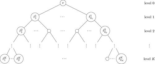
This results in time complexity of $\mathcal{O}(|V\left|\right|E|).$ Note that this complexity can be significantly improved to $\mathcal{O}(b^k),$ when we are restricting BFS trees to depths of k, where b is the branching factor (or average outdegree) of the tree. For small values of k, this reduces to linear time complexity and it empirically makes an immense difference.

3.2. General framework of heuristic

The proposed heuristic algorithm consists of three components: an initial solution generation procedure, a backbone-based crossover and a centrality-based neighbourhood search procedure. The algorithm begins with generation of centrality-based solutions. An improved offspring solution is generated from the centrality-based solutions by a backbone-based crossover (Subsection 3.4). This offspring solution is further improved by a centrality-based neighbourhood search procedure (Subsection 3.5). A pseudocode of the general framework of the proposed algorithm is presented in Algorithm 1. Its three components are described and explained in the subsequent sections.

3.3. Initial solution generation

The proposed algorithm begins with construction of initial feasible solutions using three centrality metrics. The first is the popular degree centrality where nodes are ranked according to their degrees. The other two measures could be seen as specialised adaptations of the Katz and betweenness centralities. The first which we refer to as $k-$Katz centrality ranks nodes according to the size of the k-depth breath first search (BFS) tree rooted at each node. The last centrality metric which we refer to as k-betweenness ranks nodes according to the number of their direct offspring summed over all generated k-depth BFS trees. We refer the interested reader to Paton et al. (2017) for detailed discussion and a numerical analysis of centrality measures.

Algorithm 1.

The proposed heuristic algorithm for DCNP

1: Input: Graph $G=(V,E)$, an integer B

2: Output: the best solution $S^{*}$ found //construct initial centrality-based solutions, Subsection 3.3

3: $P^0=\left\{C_1,C_2,C_3\right\}\leftarrow$ centralitysolution()

4: $S^{*}=\text{argmin}\left\{f(C_1),f(C_2),f(C_3)\right\}$ //generate offspring solution, Subsection 3.4

5: $S^1\leftarrow$ backboneCrossover$(C_1,C_2,C_3)$ //perform local search, Subsection 3.5

6: $S^{+}\leftarrow$ neighbourhoodSearch$(S^1)$

7: if $f(S^{+})\hspace{0.17em}<\hspace{0.17em}f(S^{*})$ then

8: $S^{*}=S^{+}$

9: end if

Let v be an arbitrary node in a graph, we summarise the centrality definitions as follows:

Definition 1

(degree centrality). The degree of a node v is the number of edges incident on v, i.e. the number of direct neighbours of v.

Definition 2

($k-$Katz centrality). The $k-$Katz of v is the number of nodes reachable from v at a hop distance less than or equal to k.

Definition 3

($k-$betweenness centrality). The $k-$ betweenness of v is the number of direct offsprings of v summed across all generated k-depth BFS trees.

Let ${\mathcal{R}}_1,{\mathcal{R}}_2,$ and ${\mathcal{R}}_3$ denote three different collections of all nodes in the input graphs ordered according to the three defined centrality measures. From each of these collections, we generate three feasible centrality-based solutions ${\mathcal{C}}_1,{\mathcal{C}}_2,$ and ${\mathcal{C}}_3$ through a probabilistic selection of B nodes. For example, to generate ${\mathcal{C}}_1,$ we sequentially add each node in ${\mathcal{R}}_1$ into ${\mathcal{C}}_1$ with probability p = .90 until the required budget is attained. We also extend the budget value by a certain number, $ϵ=\text{max}(5,0.2B),$ and then, select the next ϵ top nodes in each of ${\mathcal{R}}_1,{\mathcal{R}}_2,$ and ${\mathcal{R}}_3.$ The union of these extended budget solutions which we denote by $X_{ϵ}$ is used in the backbone crossover phase (details in Subsection 3.4).

3.4. Backbone-based crossover

Our notion of backbone crossover is similar to the double backbone crossover introduced by Zhou et al. (2018) in the sense that the offspring solution inherits elements that are common to its parent solutions as well as exclusive elements. However, our backbone procedure differs from that of Zhou et al. (2018) primarily in the number of parent solutions used. Second, our procedure for repairing a partial offspring solution combines both greedy and random node selection. This combination of greedy and random selection can be seen as a double-edged sword that intensifies and diversifies the node selection. The motivation for the use of three rather than two parent solutions is to limit the members of the partial solution inherited from the parent solutions to only promising nodes. This is potentially useful in arriving at high quality offspring solutions leading to fewer iterations of local search to converge to local optimum. For the backbone crossover, we divide the elements of the centrality-based solutions into sets as follows:

Definition 4

(3-parent elements). These consist of the intersection of all three centrality solution sets, denoted as $X_1={\mathcal{C}}_1\cap {\mathcal{C}}_2\cap {\mathcal{C}}_3.$

Definition 5

(2-parent elements). These consist of elements that are only present in exactly two parent solutions denoted as $X_2=(({\mathcal{C}}_1\cap {\mathcal{C}}_2)\cup ({\mathcal{C}}_1\cap {\mathcal{C}}_3)\cup ({\mathcal{C}}_2\cap {\mathcal{C}}_3))\setminus X_1.$

Definition 6

(1-parent elements). These consist of elements that are only present in exactly one parent solution denoted as $X_3=({\mathcal{C}}_1\cup {\mathcal{C}}_2\cup {\mathcal{C}}_3)\setminus (X_2\cup X_1).$

Definition 7

(0-parent elements). These consist of elements in the extended budget solutions denoted by $X_{ϵ}.$

The backbone crossover procedure proceeds as follows: An offspring solution S¹ is constructed by first inheriting all elements common to its parent solutions that is $S^1\leftarrow X_1.$ If $\left|S^1\right|<B,$ we repair S¹ by sequentially adding elements from sets X₂, X₃, $X_{ϵ}$ until the budget is satisfied. At each iteration of the repair process, a new node is selected into the offspring solution by one of greedy or random approaches according to some specified probabilities P_greedy and P_random. The greedy approach entails selecting a node $u\notin S^1$ which gives the best improvement to the current objective function value $f(S^1),$ i.e. $u=\text{argmax}\{f(S^1)-f(S^1\cup \left\{v\right\})\},\forall v\in (X_2\cup X_3\cup X_{ϵ})\setminus S^1.$ The random approach uses specified probabilities p₂, p₁, or p₀ to determine which of the sets X₂, X₃, or $X_{ϵ}$ from which a node is to be chosen at random.

3.5. Centrality-based neighbourhood search

We explore the neighbourhoods of the solution realised from the construction phase with the aim of arriving at the optimal solution in the region. We discuss next the neighbourhood structure as well as the node swap technique defined for our study.

Algorithm 2.

Centrality-based neighbourhood search

1: Input: a starting solution S, centrality-based neighbourhood N_s

2: Output: the best solution $S^{*}$ found

3: $S^{*}\leftarrow S$

4: $\mathit{iterCnt}\leftarrow 0$

5: while iterCnt < maxIter and $N_s\ne$ Ø do

6:    $v\leftarrow N_s.\mathit{remove}()$

7:   $S\leftarrow S\cup \left\{v\right\}$

8:    $u\leftarrow {\text{argmin}}_{w\in S}\left\{f(S\setminus \left\{w\right\})-f(S)\right\}$

9: $\mathrm{\hspace{1em}S}\leftarrow S\setminus \left\{u\right\}$

10: if $f(S)\hspace{0.17em}<\hspace{0.17em}f(S^{*})$ then

11:    $S^{*}\leftarrow S$

12:    $\mathit{iterCnt}\leftarrow 0$

13:  else

14:    $\mathit{iterCnt}\leftarrow \mathit{iterCnt}+1$

15:  end if

16: end while

3.5.1. Centrality-based neighbourhood structure

Considering the time complexity for evaluation of a candidate solution, the traditional neighbourhood which swaps each node $v\in S$ with a node $u\in V\setminus S$ requires a time of $\mathcal{O}(B(\left|V\right|-B)(\left|V\right|\left|E\right|))$ to evaluate all neighbourhood solutions. This becomes prohibitive when $\left|V\right|$ is very large or when many local search iterations are required. To mitigate this computational burden, we design a much smaller alternative neighbourhood. Let s be a positive integer corresponding to the size of each centrality-based neighbourhood. Thus, our centrality based neighbourhood N_s for a given solution S consists of the union of the top s nodes ranked according to the three defined centrality measures in the residual graph $G[V\setminus S].$ Similar to the generation of centrality-based solutions, the top ranking nodes in each centrality measure have a 90% chance of being selected into the corresponding centrality neighbourhood. The cardinality of N_s is bounded below and above by s and 3s. Hence, the size of the neighbourhood is reduced to $(B|N_s|).$

3.5.2. Two-phase node swap

We employ the two-phase node exchange strategy used in Zhou et al. (2018). In keeping with its name, the two-phase node exchange strategy is composed of two separate phases: a “removal phase” which removes a node from the resultant subgraph and an “add phase” which adds a node back to the subgraph. At each iteration of the two-phase node exchange strategy, a node is removed from the neighbourhood and added into the current solution S. This makes S infeasible. The second phase repairs this infeasibility by identifying a node $v\in S$ which results in the minimum increase in the objective function value, v is then added back to the subgraph.

4. Computational studies

4.1. Test instances

Our computational experiments were based on both real-world and synthetic network instances. The real-world instances consists of a subset of networks from the Pajek and UCINET dataset (Batagelj & Mrvar, 2006; UCINET Software Datasets, n.d.). The first set of synthetic instances consist of Barabasi–Albert, Erdos–Renyi, and uniform random graphs which were generated using NetworkX random graph generators (Hagberg et al., 2008). Characteristics of the real-world and NetworkX-generated instances are summarised in Tables 1 and 2. Detailed descriptions of these network instances and how to get them are available in the Online Supplementary Information.

Table 1. Characteristics of real world graph instances.

Graph	n	m	Diam	% k-Conn
Hi-tech	33	91	5	88.3
Karate	34	78	5	85.6
Mexican	35	117	4	98.0
Sawmill	36	62	8	63.0
Chesapeake	39	170	3	100.0
Dolphins	62	159	8	58.5
Lesmiserable	77	254	5	85.4
Santafe	118	200	12	32.9
Sanjuansur	75	155	7	48.7
Attiro	59	128	8	68.0
LindenStrasse	232	303	13	12.1
SmallWorld	233	994	4	95.2
NetScience	379	914	17	13.3
USAir97	332	2126	6	84.8

Table 2. Characteristics of NetworkX-generated synthetic graph instances.

Graph	n	m	Diam	Density (%)	% k-Conn
ba1	100	475	4.0	9.6	99.9
ba2	100	900	3.0	18.0	100
er1	80	470	3.0	14.9	100
er2	200	1004	4.0	5.0	97.7
gnm1	200	1000	4.2	5.0	97.9
gnm2	300	1500	4.4	3.3	94.1
gnm3	300	2000	4.0	4.5	99.6

The other set of synthetic networks include instances from the benchmark networks in Ventresca (2012). Since, these benchmark instances were generated for the traditional pairwise- connectivity CNP and not the distance-based connectivity CNP, only 2 (13%) of these instances have % k-Conn greater than 20%. We use these two instances (labelled as FF250 and WS250a in Table 6) and generate additional instances of similar size and order as the original benchmark networks in Ventresca (2012).

4.2. Experimental settings

Our computational study was performed on an HP computer equipped with Windows 8.1 × 64 operating system, an Intel Core i3-4030 processor(CPU 1.90 GHz) and RAM 8GB. The proposed algorithms were implemented in Python 3.6 (Anaconda 5). We used NetworkX (Hagberg et al., 2008) for random graph generation and manipulating of the graphs. In the design of the proposed algorithm, some parameters were selected for our computational experiments. We executed several preliminary experiments to select most of these parameters. Final values of the parameters used in the computational results presented in this article are summarised in Table 3. All experiments were run with a time limit of 3600 s. In line with previous studies, we also set hop distance threshold k = 3 which is reasonable since most of the tested instances have a large proportion of nodes connected within this hop distance.

Table 3. Parameter settings for computational experiments.

Parameter	Description	Values
ϵ	extended budget limit for centrality solution	Max (5, 0.2 B)
s	size of each centrality-based neighborhood	$B+ϵ$
maxIter	maximum no of improvement iteration	100
Pgreedy	probability of greedy node selection in any crossover iteration	0.7
Prandom	probability of random node selection in any crossover iteration	0.3
p2	probability of random node selection from set X2	0.5
p1	probability of random node selection from set X3	0.3
p0	probability of random node selection from set $X_{ϵ}$	0.2

4.3. Performance of the heuristic algorithm

We present results obtained from the proposed heuristic algorithm for different graph instances. The results have been summarised from ten independent runs for each instance. Values reported in the tables include objective function values minimum (min), mean (avg), maximum (max), and standard deviation (SD) for the proposed heuristic algorithm, as well as optimal objective function values (Opt) or best lower bounds (LB) and best upper bounds (UB) realised from Gurobi solver 8.1.0 (Gurobi Optimization, 2016). The reported optimal objective function values or best lower and upper bounds were generated using the integer programming models in Veremyev et al. (2015) and Alozie et al. (2021). Computational times (in seconds) for both exact and heuristic algorithms are also reported in columns labelled respectively by t_exact and t_heur with the smaller run time highlighted in bold. Exact optimal (Opt) or best upper bounds (UB) are compared with heuristic minimum objective values (min).

4.3.1. Real-world instances

Results for the real world instances are summarised in Table 4, where we observe that the proposed heuristic attains the optimal objective values for all 28 instances. Also the average and maximum objective function values obtained by the heuristic matches the optimal solution for 16 of the instances (see when SD = 0.0 in Table 4).

Table 4. Results for Real-world instances: Optimal value of objective function (Opt) and summary results for heuristic (minimum (min), mean (avg), maximum (max), and standard deviation (SD)) for budget settings $B=(0.05\mathrm{n},0.1\mathrm{n}).$

	B = 0.05 n							B = 0.1 n
Graph	Opt	t_exact	min	avg	max	SD	t_heur	Opt	t_exact	min	avg	max	SD	t_heur
Hi-tech	397	0.12	397	397.0	397	0.0	0.2	293	0.59	293	294.8	297	1.9	0.5
Karate	324	0.13	324	324.0	324	0.0	0.2	147	0.11	147	150.9	186	11.7	0.4
Mexican	527	0.23	527	527.0	527	0.0	0.3	358	0.33	358	358.0	358	0.0	0.6
Sawmill	215	0.06	215	215.0	215	0.0	0.2	135	0.08	135	135.0	135	0.0	0.2
Chesapeake	696	0.6	696	696.0	696	0.0	0.3	512	1.18	512	515.2	528	6.4	1.1
Dolphins	820	1.03	820	820.0	820	0.0	1.3	583	1.71	583	591.7	616	13.4	2.5
Lesmiserable	930	0.52	930	930.0	930	0.0	1.9	323	0.97	323	323.0	323	0.0	2.9
Santafe	305	0.2	305	305.0	305	0.0	1.2	116	0.59	116	116.0	116	0.0	2.8
Sanjuansur	803	0.35	803	803.0	803	0.0	0.9	457	0.39	457	457.2	459	0.6	2.0
Attiro	743	0.31	743	743.0	743	0.0	0.5	444	0.61	444	450.4	474	10.3	0.7
LindenStrasse	1054	1.34	1054	1057.8	1090	10.7	5.9	429	2.82	429	431.7	445	4.6	12.7
SmallWorld	4629	202.87	4629	4660.5	4734	48.1	51.4	1694	117.54	1694	1694.0	1694	0.0	58.6
NetScience	2102	9.07	2102	2102.0	2102	0.0	52.9	897	7.12	897	901.0	927	8.8	112.3
USAir97	10,623	377.83	10,623	10,697.2	10,729	48.6	269.7	3100	1277.38	3100	3219.1	3405	105.9	423.6

Values compared are Opt and min, lower values are better (best in bold).

4.3.2. Synthetic instances

Results for our first set of synthetic networks are summarised in Table 5 as well as Figures 2–5. Overall, the heuristic attains the best known upper bounds in 16.7% of the instances, yielding new upper bounds in 57.1% but falls short of the best UB in 26.2% of the instances (see Figure 2).

Figure 2. Summary results of heuristic algorithm compared with exact over synthetic instances.

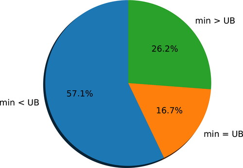
Figure 3. Comparison of gaps from best UB and Heuristic for the synthetic instances, B = 0.05 n.

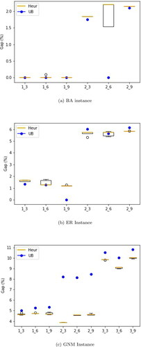
Figure 4. Comparison of gaps from best UB and Heuristic for the synthetic instances, B = 0.1 n.

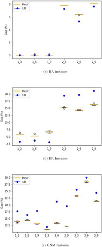
Figure 5. Variation of average percentage improvement in objective function values following the neighbourhood search procedure across different synthetic network types; budget settings $B=0.05\mathrm{n}$ and $0.1\mathrm{n}.$

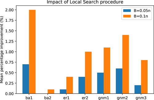
Table 5. Results for synthetic instances: Exact Lower and Upper bounds (LB, UB) and summary statistics for heuristic (minimum (min), mean (avg), maximum (max), and standard deviation (SD)) for budget settings $B=(0.05\mathrm{n},0.1\mathrm{n}).$

	B = 0.05 n								B = 0.1 n
Graph	LB	UB	t_exact	min	avg	max	SD	t_heur	LB	UB	t_exact	min	avg	max	SD	t_heur
ba1(3)	4275.0	4275	330.19	4275	4275.0	4275	0.0	8.5	3330	3330	278.57	3330	3330.0	3330	0.0	13.6
ba1(6)	4278.0	4278	303.56	4278	4278.4	4282	1.2	9.8	3390	3390	476.99	3390	3391.0	3395	2.0	14.1
ba1(9)	4193.0	4193	169.48	4193	4193.0	4193	0.0	7.7	3328	3328	374.92	3328	3328.4	3332	1.2	13.6
ba2(3)	4384.2	4461	3600	4465	4465.0	4465	0.0	20.9	3716.0	3987	3600	4005	4005.0	4005	0.0	46.1
ba2(6)	4369.0	4369	562.95	4436	4453.4	4465	14.2	19.3	3717.5	3916	3600	3955	3955.9	3956	0.3	44.5
ba2(9)	4371.4	4463	3600	4465	4465.0	4465	0.0	18.3	3702.2	3986	3600	4004	4004.0	4004	0.0	48.6
er1(3)	2798.0	2835	3600	2842	2843.4	2845	1.2	9.6	2394.6	2474	3600	2535	2538.7	2549	5.0	20.5
er1(6)	2799.4	2835	3600	2835	2839.6	2848	5.7	11.2	2394.7	2482	3600	2485	2519.1	2540	12.8	22.9
er1(9)	2814.0	2814	1787.2	2847	2847.7	2850	0.9	8.4	2378.4	2452	3600	2528	2539.0	2548	6.0	20.6
er2(3)	15,989.5	16,955	3600	16,842	16,897.3	16,909	19.9	101.5	12,468.9	14,886	3600	14,332	14,360.0	14,385	14.0	213.5
er2(6)	16,025.5	16,930	3600	16,887	16,930.0	16,960	28.6	91.5	12,575.4	15,052	3600	14,364	14,380.2	14,403	11.9	217.2
er2(9)	15,969.7	16,954	3600	16,899	16,900.9	16,908	3.4	129.1	12,414.4	15,038	3600	14,397	14,434.0	14,488	24.1	255.7
gnm1(3)	15,972.3	16,771	3600	16,706	16,716.6	16,740	9.3	136.4	12,516.5	14,730	3600	14,193	14,256.3	14,296	31.2	252.2
gnm1(6)	16,209.4	17,062	3600	16,975	16,977.4	16,987	3.5	104.6	12,600.7	14,658	3600	14,399	14,419.0	14,446	13.4	221.4
gnm1(9)	16,099.0	16,958	3600	16,843	16,860.1	16,886	15.9	89.0	12,564.9	14,803	3600	14,195	14,211.3	14,221	12.0	178.1
gnm2(3)	34,014.7	36,803	3600	35,332	35,334.7	35,341	4.1	281.4	25,876.6	28,978	3600	28,715	28,734.4	28,764	21.0	637.4
gnm2(6)	33,700.6	36,445	3600	35,236	35,245.4	35,252	6.0	303.4	25,261.7	30,635	3600	28,554	28,629.7	28,704	48.5	647.9
gnm2(9)	33,782.3	36,641	3600	35,331	35,350.8	35,388	18.8	353.9	25,765.4	30,805	3600	28,868	28,922.1	28,956	25.0	709.9
gnm3(3)	36,402.9	40,229	3600	39,978	39,982.0	39,983	2.0	627.3	28,541.1	35,847	3600	35,158	35,198.5	35,238	25.0	1539.6
gnm3(6)	36,557.1	40,217	3600	39,848	39,876.1	39,902	18.8	681.6	27,307.3	35,501	3600	35,000	35,079.6	35,176	47.9	1353.8
gnm3(9)	36,258.1	40,176	3600	39,852	39,880.5	39,896	14.8	605.1	28,697.9	35,704	3600	34,785	34,837.7	34,935	50.7	1323.1

Values compared are UB and min, lower values are better (best in bold).

From Figures 3 and 4, we can observe that for the instances where the heuristic falls short, the quality of the solutions is still competitive in comparison to the best UB.

Analysing the performance of the heuristic across the synthetic network classes, we observed that the effectiveness of the heuristic framework is more pronounced in the less dense instances within each random network class. For example, for both Barabasi–Albert and Erdos–Renyi classes, the heuristic yields new upper bounds in all of the less-dense instances in both classes (see results for ba1 and er2 instances in Table 5).

However, as the edge density increases (graph characteristics are shown in Table 2), the heuristic falls short of the best known upper bounds matching only 1 out of the 6 er1 instances and falling short in all ba2 instances. This behaviour might be explained by the concept of “Structural Equivalence” wherein some of the most central nodes have overlapping neighbourhoods leading to redundancy of the solution set in which they occur (Borgatti, 2006). Moreover, ba2 and er1, being highly connected networks, are likely to suffer from the” Problem of Ties” which affects the performance of centrality-based algorithm on such topological structures (Ventresca & Aleman, 2015). Our empirical investigation correlates with the above concepts. We observed the existence of multiple solutions with similar objective value differing only by one or two nodes. Thus, based on the structure of the centrality-based neighbourhood, the node swapping technique yielded little or no improvement as could be seen from the heights of the bars for ba2 and er1 in Figure 5. The bars in Figure 5 represent percentage improvement calculated based on the objective function values realised before and after local search (InitialObj and FinalObj, respectively) averaged across all instances in each of the displayed synthetic graph type.

For a given problem instance, the percentage improvement is calculated as $$\%\text{improvement}=100\mathrm{·}\frac{\text{InitialObj}-\text{FinalObj}}{\text{InitialObj}}\%$$ and averaged over all 10 runs of the instance. Across the three random network classes, the heuristics performed best in the uniform random network class, yielding new upper bounds in all 18 instances with all maximum objective values even less than the exact upper bounds. From Figure 5, the impact of the local search procedure is observed to significantly improve solutions obtained in all these instances. This is also the case for the less-dense Barabasi–Albert and Erdos–Renyi (ba1, er2) instances where the heuristic objective values were at least as good as the exact upper bounds. The instances in the uniform random graph class were the most challenging for the exact algorithms. Hence, achieving these new upper bounds shows the usefulness of the proposed algorithm in providing good solution for challenging problem instances. Overall we also observed that classes and instances of the random graphs that were challenging for the exact algorithms were also the most computationally intensive for the heuristic algorithm as can be seen in average computational times reported for the uniform random graphs on Table 5. Also, the impact of the local search procedure increases with increase in the budget setting B as would be expected since the size of the neighbourhood is directly proportional to B.

4.3.3 Benchmark instances

We extend our computational experiment to the set of benchmark synthetic graphs which have been used as test instances for most heuristic algorithms developed for the classical critical node detection problem.

Due to the sparsity of these networks, we focused only on instances where the initial percentage k-distance connectivity (k-Conn%) is greater or equal to 20% (labelled as FF250 and WS250a in Table 6). From Table 6, we observe that the heuristics realises the exact optimal objective value for 3 out 12 of the instances and yields new upper bounds in the remaining nine instances. We also observed that as the budget increases especially for large dense graphs, the heuristic algorithm struggles to terminate within the specified time limit.

Table 6. Results for benchmark synthetic instances: Exact Lower and Upper bounds (LB, UB) and summary statistics for heuristic (minimum (min), mean (avg), maximum (max), and standard deviation (SD)).

					Exact			Heur
Graph	n	m	k-Conn (%)	B	LB	UB	t_exact	min	avg	max	SD	t_heur
FF250	250	514	23.9	13	1587.0	1587	11.44	1587	1598.2	1601	5.6	16.7
BA250	250	1225	98.08	25	13,772.0	13,772	3160.27	13,722	13,788.25	13,811	16.89	137.6
BA500	500	2475	95.18	50	24,847.0	24,847	3331.03	24,847	24,847	24,847	0	1104.7
BA1000	1000	4975	84.97	100	16,071.326	316,735	3600	59,178	60,488.9	62,487	909.7	3600.0
ER250	250	1190	94.04	25	17,958.996	22,288	3600	19,894	19,931.6	19,970	19.89	326.45
ER500	500	2570	86.27	50	30,845.690	79,482	3600	68,062	68,129.2	68,208	39.43	3189.6
ER1000	1000	5061	64.66	100	70,494.315	221,831	8052	173,538	174,326.1	175,494	527.5	3600.0
WS250a	250	1246	52.9	70	1038.980	2319	3600	2034	2056.8	2093	17.0	728.7
WS250b	250	1250	79.65	25	14,586.020	15,223	3600	15,020	15,044.67	15,086	16.55	316.1
WS500	500	2500	69.35	50	25,907.377	53,729	3600	51,460	51,567.2	51,659	63.2	3483.39
GNM250	500	1250	96.17	25	18,638.331	22,711	3600	20,967	20,984.5	21,013	17.0	453.8
GNM500	1000	2500	84.74	50	29,461.785	78,001	3600	65,775	65,892.9	65,975	67.1	2883.02

Budget settings for each instance are specified in column labelled B. Values compared are UB and min, lower values are better (best in bold).

In particular for BA1000 and ER1000, the heuristic algorithm was unable to terminate within the specified time limit. These two instances were also the most challenging for the exact algorithm as seen from the gaps between the upper and lower bounds especially for ER1000 for which an upper bound was only achieved after 8052 s. A possible way to enhance the computational burden of the proposed heuristic for the larger instances might be to increase the probability of using a randomised node selection when repairing the partial offspring solution. However, the quality of the offspring solution might be affected in which case local search improvement can be employed with the gained time. Also an approximate evaluation of objective change might be employed during iterations of the greedy backbone crossover and the local search to reduce the computational burden of solution evaluation.

4.4. Two-parent versus three-parent backbone crossover

We conclude the discussion on computational experiments by comparing the proposed three-parent backbone crossover to a two-parent approach. Recall that three initial feasible solutions are generated based on three centrality measures which are all used to generate offspring solutions (see Subsections 3.3 and 3.4). We compare this to a two-parent approach in which we randomly select two out of the initial solutions as was done in Zhou et al. (2018). Using the two selected parent solutions, we construct an offspring solution using a combination of greedy and random backbone crossover. Specifically, the initial offspring solution is repaired using the greedy approach 70% of the time and the random approach 30% of the time just as with the three-parent approach. The random approach selects from the corresponding 1-parent elements or 0-parent elements based on probabilities 0.6 and 0.4, respectively. Comparative performance of the proposed three-parent backbone crossover and its alternative two-parent in terms of the minimum objective value (min) and mean objective value (avg) are displayed in Figure 6(a,b), respectively. The x-axis represents the instances while the y-axis represents the percentage gap between the objective values (minimum values and mean values) realised by the heuristic and the exact upper bounds (UB). The percentage gaps are calculated as $$\%\text{gap}=100·\frac{\text{obj}-\text{UB}}{\text{obj}}\%$$ where obj is the minimum or mean objective value. A gap less than zero implies that the heuristic approach (three-parent or two-parent) realises a new upper bound for the given instance.

Figure 6. Comparison of three-parent and two-parent backbone crossover approaches.

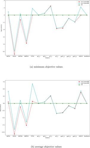
From Figure 6 and Table 7, we observe that the three-parent approach obtains better minimum and mean objective values, respectively, for 10 instances and 9 instances out of the 14 tested instances. On the other hand, the two-parent approach obtains better minimum and mean objective values, respectively, in 1 instance and 2 instances. Both approaches perform alike obtaining the same minimum and mean objective values respectively for the smaller Barabasi–Albert instances (ba1_3, ba2_3) as well as the Smallworld instance. The advantage of the three-parent approach is more pronounced for the tested benchmark instances which spans all the random graph class. We observed that while the three-parent approach yields three new upper bounds and achieves the exact optimal for two of the five tested benchmark instances, the two-parent approach obtains minimum objective values which are worse than the exact upper bounds. Actual minimum and mean objective values along with run times for both three-parent and two-parent backbone crossover can be seen in Table 7.

Table 7. Comparison of the proposed heuristics using three-parent and two-parent backbone crossover approaches on a set of test instances, $B=0.1\mathrm{n}$ except for FF250 where B = 13 as recorded from the source of the data.

					Three-parent			Two-parent
Graph	n	m	k-Conn (%)	UB	min	avg	t_heur	min	avg	t_heur
SmallWorld	233	994	95.2	1694	1694	1694	58.6	1694	1694	45.6
USAir97	332	2126	84.8	3100	3100	3219.1	423.6	3168	3232.4	293.5
ba1_3	100	475	99.9	3330	3330	3330.0	13.6	3330	3330.0	13.8
ba2_3	100	900	100	3987	4005	4005.0	46.1	4005	4005.0	42.9
er1_3	80	470	100	2474	2535	2538.7	20.5	2534	2540.7	17.75
er2_3	200	1004	97.7	14,886	14,332	14,360.0	213.5	14,348	14,370.4	183.9
gnm1_3	200	1000	97.9	14,730	14,193	14,256.3	252.2	14,244	14,249.8	196.3
gnm2_3	300	1500	94.1	28,978	28,715	28,734.4	637.4	28,718	28,729.8	568.1
gnm3_3	300	2000	99.6	35,847	35,158	35,198.5	1539.6	35,171	35,235.0	1353.5
BA250	250	1225	98.08	13,722	13,722	13,788.3	137.6	13,844	14,292.3	165.62
ER250	250	1190	94.04	22,288	19,894	19,931.6	326.45	20,107	20,275.8	263.99
WS250b	250	1250	79.65	15,223	15,020	15,044.7	316.1	15,275	15,370.3	211.46
GNM250	250	1250	96.17	22,711	20,967	20,984.5	453.8	21,088	21,253.1	431.09
FF250	250	514	23.9	1587	1587	1598.2	16.7	1615	1694.2	16.2

Values compared are minimum (min) and mean (avg) objective values obtained from both approaches as well as run times (t_heur), lower values are better (best in bold). The exact upper bounds are given in column labelled UB.

Overall, the results indicate that the three-parent approach performs better than the two-parent approach in terms of minimum and mean objective values howbeit at higher cost of run times. This could be attributed to the higher number of iterations of the greedy procedure required to complete the initial offspring solution obtained from the common elements of all three parents. An approximate method to evaluate changes in objective value changes within the greedy procedure could be useful to improve the run times.

5. Conclusion

In this study, we considered a class of distance-based critical node detection problem. The proposed heuristic algorithm generates good solutions following a combination of greedy and randomised backbone-based crossover on initial feasible solutions. We also presented an improvement scheme that is derived from a centrality-based neighbourhood search. Extensive computational experiments on both real-world and synthetic graphs show the usefulness of the developed heuristics in generating good solutions when compared to exact solutions particularly for challenging problem instances. In the future, it will be interesting to develop more efficient neighbourhoods to overcome the problem of ties inherent in edge-dense instances of the Barabasi–Albert and Erdos–Renyi network classes. It will also be useful to extend the proposed framework to other classes of the distance-based critical node problem. Given the computational burden of evaluating feasible solutions of the DCNP for larger instances, an alternative scheme for solution evaluation is an interesting future problem.

Acknowledgement

We also thank two anonymous referees for their insightful comments that helped improve the exposition of the article.

Disclosure statement

No potential conflict of interest was reported by the authors.

Additional information

Funding

This material is based upon work supported by the Air Force Office of Scientific Research under award number FA9550-17-1-0029.

References

- Addis, B., Di Summa, M., & Grosso, A. (2013). Identifying critical nodes in undirected graphs: Complexity results and polynomial algorithms for the case of bounded treewidth. Discrete Applied Mathematics, 161(16–17), 2349–2360. https://doi.org/https://doi.org/10.1016/j.dam.2013.03.021
- Aickelin, U., & Clark, A. (2011). Heuristic optimisation. Journal of the Operational Research Society, 62(2), 251–252. https://doi.org/https://doi.org/10.1057/jors.2010.160
- Alozie, G. U., Arulselvan, A., Akartunali K., & Pasiliao, E. (2021). Efficient methods for the distance-based critical node detection problem in complex networks. Computers & Operations Research, 131, 105254. https://doi.org/https://doi.org/10.1016/j.cor.2021.105254
- Aringhieri, R., Grosso, A., Hosteins, P., & Scatamacchia, R. (2016a). A general evolutionary framework for different classes of critical node problems. Engineering Applications of Artificial Intelligence, 55, 128–145. https://doi.org/https://doi.org/10.1016/j.engappai.2016.06.010
- Aringhieri, R., Grosso, A., Hosteins, P., & Scatamacchia, R. (2016b). Local search metaheuristics for the critical node problem. Networks, 67(3), 209–221. https://doi.org/https://doi.org/10.1016/j.engappai.2016.06.010
- Aringhieri, R., Grosso, A., Hosteins, P., & Scatamacchia, R. (2016c). A preliminary analysis of the distance based critical node problem. Electronic Notes in Discrete Mathematics, 55, 25–28. https://doi.org/https://doi.org/10.1016/j.endm.2016.10.007
- Aringhieri, R., Grosso, A., Hosteins, P., & Scatamacchia, R. (2019). Polynomial and pseudo-polynomial time algorithms for different classes of the distance critical node problem. Discrete Applied Mathematics, 253, 103–121. https://doi.org/https://doi.org/10.1016/j.dam.2017.12.035
- Arulselvan, A., Commander, C. W., Elefteriadou, L., & Pardalos, P. M. (2009). Detecting critical nodes in sparse graphs. Computers & Operations Research, 36(7), 2193–2200. https://doi.org/https://doi.org/10.1016/j.cor.2008.08.016
- Arulselvan, A., Commander, C. W., Pardalos, P. M., & Shylo, O. (2007). Managing network risk via critical node identification. In Risk management in telecommunication networks. Springer.
- Arulselvan, A., Commander, C. W., Shylo, O., & Pardalos, P. M. (2011). Cardinality-constrained critical node detection problem. In Performance models and risk management in communications systems (pp. 79–91). Springer.
- Batagelj, V., & Mrvar, A. (2006). Pajek datasets. http://vlado.fmf.uni-lj.si/pub/networks/data/
- Boginski, V., & Commander, C. W. (2009). Identifying critical nodes in protein-protein interaction networks. In Clustering challenges in biological networks (pp. 153–167). World Scientific.
- Borgatti, S. P. (2006). Identifying sets of key players in a social network. Computational & Mathematical Organization Theory, 12(1), 21–34. https://doi.org/https://doi.org/10.1007/s10588-006-7084-x
- Di Summa, M., Grosso, A., & Locatelli, M. (2012). Branch and cut algorithms for detecting critical nodes in undirected graphs. Computational Optimization and Applications, 53(3), 649–680. https://doi.org/https://doi.org/10.1007/s10589-012-9458-y
- Gurobi Optimization, I. (2016). Gurobi optimizer reference manual. http://www.gurobi.com
- Hagberg, A., Swart, P., & Chult, D. S. (2008). Exploring network structure, dynamics, and function using NetworkX (Tech. Rep.). Los Alamos National Lab (LANL).
- Hooshmand, F., Mirarabrazi, F., & MirHassani, S. (2020). Efficient benders decomposition for distance-based critical node detection problem. Omega, 93, 102037. https://doi.org/https://doi.org/10.1016/j.omega.2019.02.006
- Hosteins, P., & Scatamacchia, R. (2020). The stochastic critical node problem over trees. Networks, 76(3), 321–426. https://doi.org/https://doi.org/10.1002/net.21948
- Lalou, M., & Kheddouci, H. (2019). A polynomial-time algorithm for finding critical nodes in bipartite permutation graphs. Optimization Letters, 13(6), 1345–1364. https://doi.org/https://doi.org/10.1007/s11590-018-1371-6
- Lalou, M., Tahraoui, M. A., & Kheddouci, H. (2016). Component-cardinality-constrained critical node problem in graphs. Discrete Applied Mathematics, 210, 150–163. https://doi.org/https://doi.org/10.1016/j.dam.2015.01.043
- Li, J., Pardalos, P. M., Xin, B., & Chen, J. (2019). The bi-objective critical node detection problem with minimum pairwise connectivity and cost: Theory and algorithms. Soft Computing, 23(23), 12729–12744. https://doi.org/https://doi.org/10.1007/s00500-019-03824-8
- Matisziw, T. C., & Murray, A. T. (2009). Modeling s–t path availability to support disaster vulnerability assessment of network infrastructure. Computers & Operations Research, 36(1), 16–26.
- Nandi, A. K., & Medal, H. R. (2016). Methods for removing links in a network to minimize the spread of infections. Computers & Operations Research, 69, 10–24. https://doi.org/https://doi.org/10.1016/j.cor.2015.11.001
- Naoum-Sawaya, J., & Buchheim, C. (2016). Robust critical node selection by benders decomposition. INFORMS Journal on Computing, 28(1), 162–174. https://doi.org/https://doi.org/10.1287/ijoc.2015.0671
- Paton, M., Akartunali, K., & Higham, D. J. (2017). Centrality analysis for modified lattices. SIAM Journal on Matrix Analysis and Applications, 38(3), 1055–1073. https://doi.org/https://doi.org/10.1137/17M1114247
- Purevsuren, D., Cui, G., Win, N. N. H., & Wang, X. (2016). Heuristic algorithm for identifying critical nodes in graphs. Advances in Computer Science: An International Journal, 5(3), 1–4.
- Schieber, T. A., Carpi, L., Frery, A. C., Rosso, O. A., Pardalos, P. M., & Ravetti, M. G. (2016). Information theory perspective on network robustness. Physics Letters A, 380(3), 359–364. https://doi.org/https://doi.org/10.1016/j.physleta.2015.10.055
- Shen, S., & Smith, J. C. (2012). Polynomial-time algorithms for solving a class of critical node problems on trees and series-parallel graphs. Networks, 60(2), 103–119. https://doi.org/https://doi.org/10.1002/net.20464
- Shen, S., Smith, J. C., & Goli, R. (2012). Exact interdiction models and algorithms for disconnecting networks via node deletions. Discrete Optimization, 9(3), 172–188. https://doi.org/https://doi.org/10.1016/j.disopt.2012.07.001
- Silver, E. A. (2004). An overview of heuristic solution methods. Journal of the Operational Research Society, 55(9), 936–956. https://doi.org/https://doi.org/10.1057/palgrave.jors.2601758
- UCINET Software Datasets. (n.d.). https://sites.google.com/site/ucinetsoftware/datasets/
- Ventresca, M. (2012). Global search algorithms using a combinatorial unranking-based problem representation for the critical node detection problem. Computers & Operations Research, 39(11), 2763–2775. https://doi.org/https://doi.org/10.1016/j.cor.2012.02.008
- Ventresca, M., & Aleman, D. (2015). Efficiently identifying critical nodes in large complex networks. Computational Social Networks, 2(1), 6. https://doi.org/https://doi.org/10.1186/s40649-015-0010-y
- Ventresca, M., Harrison, K. R., & Ombuki-Berman, B. M. (2018). The bi-objective critical node detection problem. European Journal of Operational Research, 265(3), 895–908. https://doi.org/https://doi.org/10.1016/j.ejor.2017.08.053
- Veremyev, A., Boginski, V., & Pasiliao, E. L. (2014). Exact identification of critical nodes in sparse networks via new compact formulations. Optimization Letters, 8(4), 1245–1259. https://doi.org/https://doi.org/10.1007/s11590-013-0666-x
- Veremyev, A., Prokopyev, O. A., & Pasiliao, E. L. (2014). An integer programming framework for critical elements detection in graphs. Journal of Combinatorial Optimization, 28(1), 233–273. https://doi.org/https://doi.org/10.1007/s10878-014-9730-4
- Veremyev, A., Prokopyev, O. A., & Pasiliao, E. L. (2015). Critical nodes for distance-based connectivity and related problems in graphs. Networks, 66(3), 170–195. https://doi.org/https://doi.org/10.1002/net.21622
- Walteros, J. L., Veremyev, A., Pardalos, P. M., & Pasiliao, E. L. (2019). Detecting critical node structures on graphs: A mathematical programming approach. Networks, 73(1), 48–88. https://doi.org/https://doi.org/10.1002/net.21834
- Wang, S., Gong, M., Liu, W., & Wu, Y. (2020). Preventing epidemic spreading in networks by community detection and memetic algorithm. Applied Soft Computing, 89, 106–118. https://doi.org/https://doi.org/10.1016/j.asoc.2020.106118
- Yadegari, E., Alem-Tabriz, A., & Zandieh, M. (2019). A memetic algorithm with a novel neighborhood search and modified solution representation for closed-loop supply chain network design. Computers & Industrial Engineering, 128, 418–436. https://doi.org/https://doi.org/10.1016/j.cie.2018.12.054
- Zhang, L., Xia, J., Cheng, F., Qiu, J., & Zhang, X. (2020). Multiobjective optimization of critical node detection based on cascade model in complex networks. IEEE Transactions on Network Science and Engineering, 7(3), 2052–2066. https://doi.org/https://doi.org/10.1109/tnse.2020.2972980
- Zhou, Y., Hao, J.-K., & Glover, F. (2018). Memetic search for identifying critical nodes in sparse graphs. IEEE Transactions on Cybernetics, 49(10), 3699–3712. https://doi.org/https://doi.org/10.1109/TCYB.2018.2848116