Is the regulatory downturn LGD adequate? Performance analysis and alternative methods

Abstract

This paper addresses the drawbacks of the macroeconomic approach to estimate downturn loss given defaults (LGD) that is currently used in the EU banking regulation. Using a large dataset of more than 186.000 defaulted credit exposures covering a time span of 18 years we demonstrate by Monte Carlo simulations that the macroeconomic approach proposed by the European Banking Authority (EBA) does not reach a confidence level of 99.9%. As an alternative we develop a downturn LGD estimation based on a latent variable approach. Our simulations demonstrate that this approach outperforms the macroeconomic approach in two dimensions: It induces capital requirements that are sufficient to cover potential losses at a 99.9% confidence level and compared to all regulatory eligible macroeconomic approaches that provide sufficient loss coverage, our approach requires the least amount of capital. The latent variable approach, developed in this paper is applicable for market based LGDs as well as for workout LGDs, i.e., for defaulted exposures with a long workout period. We argue that banking regulation as well as banks’ risk management can be improved if the latent variable approach is used in addition to the traditional macroeconomic approach for estimating downturn LGDs.

Keywords:

• Basel Accord
• Internal Ratings-Based Approach
• downturn loss given default
• systematic risk
• latent variable
• Global Credit Data

JEL CLASSIFICATION:

• G18
• G21
• G28

1. Introduction

Regulatory capital requirements for banks are designed to ensure that financial institutions’ own funds are sufficient to absorb potential losses. Under the Advanced Internal Ratings Based Approach (AIRBA), financial institutions are allowed to determine the potential unexpected credit portfolio losses from defaulted loans, by using own estimates of the exposure at default, the probability of default (PD), and the loss given default (LGD), i.e., the fraction of the exposure at default that is expected to be lost, if a default occurs. The most challenging part of calculating a portfolio credit loss is to estimate the stochastic dependencies between all loan exposures.

Under the AIRBA, this problem is solved in an elegant way for the PD by using a latent variable approach. The latent variable approach captures the idea that the occurrence of a default event depends on both, on a systematic component affecting all credit exposures and on idiosyncratic features. The unobservable latent variable represents the overall macroeconomic situation to model the systematic component. While the idiosyncratic part of the loss risk can be diversified away by holding a finely granular credit portfolio, the systematic part is decisive for determining the credit portfolio risk. In the AIRBA, systematic risk is measured as the sensitivity of each exposure to the latent variable and these sensitivities reflect at the same time the default correlations of all exposures within a credit portfolio. Stressing the latent variable to its 99.9% percentile then calculates the credit portfolio loss at its 99.9% confidence level. The latent variable approach has several advantages: First, it is not necessary to specify the exact macroeconomic conditions governing the systematic risk. Second, it allows to allocate a capital requirement to each credit exposure in accordance with its contribution to the portfolio risk, the so-called portfolio-invariance. Third, it is easy to implement in banking regulation, because it allows to express the PD conditional on the latent variable within a closed formula.

Despite its merits, the latent variable approach is not used for calculating unexpected losses with respect to the LGD. Instead, the regulatory approach laid down in the Capital Requirements Regulation (CRR) relies on the concept of a macroeconomic downturn LGD. The European Banking Authority (EBA) has recently specified the nature and severity of an economic downturn as the most severe values observed on a list of macroeconomic and credit-related factors over the last 20 years. Among these factors are GDP growth, unemployment rate, and aggregate default rates. The 20 years time span is chosen to cover approximately two economic cycles (EBA, 2018). Depending on banks’ data availability, the EBA has proposed several methods appropriate to estimate a downturn LGD (EBA, 2019). This macroeconomic approach has several drawbacks: First, the macroeconomic parameters identifying an economic downturn solely rely on intuition and lack any empirical evidence. Second, the approach does not adequately address the stochastic dependencies between the LGDs of the individual exposures as well as stochastic dependencies between LGDs and PDs. Koopman et al. (2011) report that even more than 100 macroeconomic covariates are not sufficient to replace the need for latent components. Betz et al. (2018) show that macroeconomic variables, in general, are not suitable to capture the true systematic effects when modelling LGDs. Third, the 20-year time span is incompatible with a confidence level of 99.9% normally used for regulatory purposes. Fourth, the treatment of downturn LGDs is inconsistent with the treatment of PDs in the AIRBA.

In this paper, we demonstrate the inadequateness of the downturn LGD methods proposed by the EBA. We propose a latent variable based approach for downturn LGDs that is consistent with the regulatory treatment of PDs and performs better than EBAs macroeconomic approach. Performance is measured by the ability to correctly estimate unexpected losses with respect to the LGD. More precisely, we are looking for an approach ensuring 1) that potential losses are covered by own funds at a confidence level of 99.9% (henceforth called the survival criterion) and 2) that this is achieved with a minimum of regulatory capital requirements (henceforth called the waste criterion). The waste criterion reflects that a banks average cost of capital increases with the equity ratio. Higher average cost of capital lead to higher loan interest rates, thus decreasing investments and dampening GDP growth. To foster economic development, it is therefore important that regulatory capital requirements are smart in the sense that they ensure financial stability without being too burdensome. In addition, a better estimation of unexpected losses helps financial institutions to improve their internal capital allocation.

To achieve this, the research goal of this paper can be differentiated to two steps. First, we study the relationship between the expected LGD value and the latent variable. Second, we test the performance of the macroeconomic approach and our alternative approach. The first step is in general more challenging for LGDs than for PDs. Whereas considering only the state of the economy at the time of default may be sufficient for market based recovery rates, i.e., for recoveries based on the market price at which defaulted exposures trade typically 30 days after default, the situation is more complicated for workout recovery rates, i.e., for recoveries calculated as the present value of all cash flows stemming from a defaulted exposure during the workout process. The workout process often lasts several years and during that period the state of the economy may fluctuate and can impact the potential LGD systematically. Thus, more than one time-point may be needed to model the workout LGD. The central idea is to incorporate a latent variables time series in the LGD model instead of only one latent variable.

Based on a database containing 186,000 resolved default cases between 2000 and 2017, our results confirm that the LGD sensitivities towards the latent variables vary with the default age. We then construct some basic latent variable based downturn LGD estimation methods and test their performance by Monte Carlo simulations. Our alternative method for downturn LGD can uphold the 99.9% survivability, while the EBA’s macroeconomic approach only shows an 81% survival chance. In comparison with the Foundation IRBA (FIRBA), our method likewise passes the performance test by survival chance, but it is superior in terms of waste, i.e., avoiding excessive capital requirements (our method: 16%, FIRBA: 22%).

The results of this paper are particularly interesting for policymakers and risk practitioners as well as for academics specialising in credit risk. In regard of downturn LGD, this paper shows plainly the inadequacy of the macroeconomic approach, which is an interesting observation for both, regulators and banks. We offer an alternative approach, which can be used by risk practitioners in parallel with the EBA’s macroeconomic approach as a benchmark. For policymakers, this paper contains insights useful to develop an adequate downturn LGD guideline. From the research perspective, this paper contributes further to the research of a latent variable based downturn LGD.

The remainder of this paper is structured as follows: section 2 reviews the literature with a focus on LGD models based on a latent variables approach; section 3 describes our methods, the performance test via Monte Carlo simulations, including the data description; section 4 shows the results from the given model and introduces our alternative downturn LGD models, followed by the performance comparison of our models with the FIRBA and AIRBA; and lastly, section 5 closes this paper with a discussion.

2. Review of the literature

Early attempts to model the downturn LGD with latent variables can be found for example in Frye (2000a), Frye (2000b), Pykhtin and Dev (2002), and Pykhtin (2003). The central idea of modelling LGDs by a latent variable approach is that a single common systematic factor (denoted by X) drives both, the default event and the expected LGD. Whereas the impact of X on the default event is mediated by the asset value, the impact of X on the LGD is mediated by the collateral value. The use of X is originated from the asymptotic single-risk factor (ASRF) model, which serves as the theoretical backbone for the IRBA.

Using US corporate bonds data, Frye (2000b) estimates a sensitivity of 23% with respect to the asset value and 17% with respect to the collateral value. Düllmann and Gehde-Trapp (2004) use a database containing bonds, corporate loans, and debt instruments in the US. They report $\approx$ 20% and 2%–3% for the respective sensitivities depending on the distribution assumptions. Aside from single-factor LGD models, some papers introduce multi-factor models to accommodate the demand for more model flexibility. These factors can be assumed to be independent, such as Pykhtin (2004), or with a particular dependence structure, such as Schönbucher (2001). The variations using a latent variables time-series may also assume a point-in-time dependency structure, as found in Bade et al. (2011), or an autoregressive process, as found in Betz et al. (2018).

One of the obstacles in modelling the systematic impact is to identify the relationship between expected LGD and X. This additional assumption is necessary to calculate the theoretical form of the downturn LGD. The simplest one is the linear relationship introduced by Frye (2000a), Frye (2000b), and Pykhtin and Dev (2002). The linearity implies the conditional LGD, $\mathbb{E}[LG{D}_i|X],$ to be normally distributed, if - as usually assumed - X is normally distributed. Motivated by the restriction of $LG{D}_i\ge 0,$ an exponential transformation can be used to ensure a log-normally distributed $\mathbb{E}[LG{D}_i|X],$ as can be found in Pykhtin (2003) and Barco (2007). Other suggestions include application of a beta distribution, such as work from Tasche (2004), or modelling LGD directly from PD, found in the work of Giese (2005), Hillebrand (2006), as well as Frye and Jacobs Jr (2012). Furthermore, Frye (2013) suggests that modelling the systematic risk in LGD can be replaced by modelling the default rates in LGD instead. The proposed alternatives in section 4.2 use a multilinear relationship. We argue that the fact that more than one latent variable will be used is more important than the choice of a specific relationship.

Compared to other studies in the literature, our methods are superior in two ways: 1) they are designed to be applicable under the IRBA and 2) they are tested for adequacy (in the sense of 99.9% confidence level) rather than accuracy (typically in the sense of an accuracy measure, e. g. R² in a regression analysis) using a large dataset with mixed facility type to replicate a real bank.

3. Methods and data

3.1. Methods for analysis

To accommodate a long workout duration, this paper extends the ASRF model to include more than one latent variable in regard to LGD. Let $C_{i,t_d}$ denote the recovery capability of a credit facility i. $C_{i,t_d}$ is calculated as the present value of all recoveries divided by the exposure at default. We propose that $C_{i,t_d}$ is influenced by the latent variables $X_{t_d},X_{t_d+1},\dots ,X_{t_d+T},$ where T denotes the workout duration and by $Z_i^C$ capturing the idiosyncratic component. The LGD reflects the accumulated impact of the latent variables during the whole workout duration. Inherited from the ASRF model, we assume $A_{i,t_d},$ the asset value at the time of default, to depend on the realisation of the latent variable at that time and on the idiosyncratic component $Z_i^A.$ $$\begin{array}{c}{A}_{i,t_d}=p·X_{t_d}+\sqrt{1-p^2}·Z_i^A,\hfill \\ C_{i,t_d}=q_{t_d}·X_{t_d}+\dots +q_{t_d+T}·X_{t_d+T}+\sqrt{1-\left|\right|q|{|}_2^2}·Z_i^C,\hfill \\ \text{where\hspace{0.5em}}\hfill & 0<p<1\mathrm{ }\text{and}\mathrm{ }{Z}_i^A,Z_i^C\sim \mathcal{N}(0,1).\hfill \end{array}$$

The coefficient $q=(q_{t_d},\dots ,q_{t_d+T})$ is an element inside the $(T+1)$-dimensional unit circle excluding the origin. Unlike other latent variable based models in the literature, we do not impose any assumption on how X_t and X_s depend on each other for any given year t and s. In the ASRF model, an obligor is defaulted, if its asset value falls below a certain threshold ($A_{i,t_d}<{\Phi }^{-1}(P{D}_i),$ where PD_i is the probability of default of credit facility i). A similar link can also be assumed for $C_{i,t_d}$ and the expected LGD. This paper diverges from other studies in that we do not assume a specific function for this link (see section 2).

The coefficient p describes the sensitivity of the asset value $A_{i,t_d}$ towards $X_{t_d}.$ The restriction for p to be positive reflects the assumption that financial distress causes a higher default rate. Similarly, the coefficients $q_{t_d},\dots ,q_{t_d+T}$ describe the sensitivity of $C_{i,t_d}$ towards the latent variables during the workout years. The restriction of q_t to be positive (for each t) is not necessary from a technical point of view. Especially for workout LGDs, a negative q_t cannot be ruled out for exposures with a long workout duration. To include these cases as well we refrain from restricting LGD to be positive. Furthermore, we impose no restriction on the length of the workout process because the model is intended to cover a typical bank, which may have a mixed portfolio containing exposures with workout LGDs and exposures with market-based LGDs.

To estimate p, this paper applies the maximum likelihood (ML) method similar to Frye (2000b). According to Gordy and Heitfield (2002), the ML method produces less bias (coming from lack of data) than the method of moments. The likelihood function can be derived through the theoretical distribution of the conditional PD, since $$\begin{array}{c}P{D}_X=\mathbb{P}(A_i\le {\Phi }^{-1}(P{D}_i)|X)\hfill \\ =\Phi (\frac{{\Phi }^{-1}(P{D}_i)-p·{\Phi }^{-1}(X)}{\sqrt{1-p^2}})=:g_A(X)\hfill \end{array}$$ and g_A is invertible and differentiable in X. The change-of-variable technique produces the density function of $P{D}_X=\mathbb{E}[D_i|X_{t_d}],$ which is $$\begin{array}{c}{f}_{P{D}_X}(y)=f_X(g_A^{-1}(y))·\left|\frac{d{g}_A^{-1}(y)}{dy}\right|\hfill \\ =\phi (\frac{{\Phi }^{-1}(P{D}_i)-\sqrt{1-p^2}{\Phi }^{-1}(y)}{p})·\frac{\sqrt{1-p^2}}{p}·\frac{d{\Phi }^{-1}(y)}{dy},\hfill \end{array}$$ where $\phi$ is the density function of the standard normal distribution. If the parameter PD_i is known, the estimation of p is reduced to a one-dimensional problem. The maximum of the likelihood function can be approximated numerically, which yields the estimated p. By applying the estimated p in $g_A(X),$ the implied X_t can be calculated for each year t. The coefficient q cannot be estimated with the ML method without an assumption on the dependence structure of ${(X_t)}_{t\in \mathbb{N}}.$ Without this structure and a link between $C_{i,t_d}$ and LGD, no likelihood function can be derived. To solve this issue, the coefficient q is estimated via a regression method through the realisations of ${(X_t)}_{t\in \mathbb{N}}$ and the observed average LGD at a given default year and workout duration. If the expected LGD can be approximated with a linear function of $C_{i,t_d},$ then we get: $$\begin{array}{c}\mathbb{E}\left[LG{D}_i\right|X_{t_d},\dots ,X_{t_d+T}]=\mu -\sigma (\underset{C_{i,t_d}}{\underbrace{q_{t_d}{X}_{t_d}+\dots +q_{t_d+T}{X}_{t_d+T}+\sqrt{1-\left|\right|q|{|}_2^2}{Z}_i^C}}).\hfill \end{array}$$

The OLS coefficients estimate $\widehat{\sigma q_t}.$ The coefficient q can be solved algebraically, since the variance of the residuals should be equal to ${\sigma }_{ϵ}^2:={\sigma }^2-{\sigma }^2\left|\right|q|{|}_2^2.$ Thus, $$\begin{array}{c}\widehat{\sigma }=\sqrt{{\sigma }_{ϵ}^2+\sum _{s=t_d}^{t_d+T}{\beta }_s^2}\\ \forall t:\widehat{q_t}=-\frac{{\beta }_t}{\widehat{\sigma }}.\end{array}$$

Without overcomplicating the issue, it is sufficient to test for the required 99.9% survivability of the resulted downturn LGD methodologies, whether the expected LGD can be adequately approximated with a linear function of $C_{i,t_d}$ (see section 4.2). From the perspective of adequacy, there is no need to find the true function. If it fails the test, then it is inadequate and we should consider non-linear alternatives. The choice of the linearity is motivated by its simplicity, since an overly complex function is unlikely to be adopted by regulators.

3.2. Monte Carlo simulations

The performance analysis is done via Monte Carlo simulations. A random portfolio will be drawn to represent a randomly chosen bank. The simulation tests whether the downturn LGD exceeds the realised LGD. For each year t, any parameter required to calculate a downturn LGD (or its alternative) will be calculated out-of-time, i. e. the required parameters can only be estimated using available data up to t. In our view, a loss database of five years would be the absolute minimum to calculate any decent estimate. Therefore, we evaluate the performance test only from 2005 onwards. For each iteration, 1,000 default cases are randomly drawn from the defaults population, which are resolved in the year t. The process is repeated 10,000 times.

This article introduce two concepts for performance measurement: the institution’s survival chance and waste. In the LGD context, an institution survives LGD-wise if the downturn LGD at t given the portfolio composition at t is at least as high as the realised LGD for all defaults resolved at t on the portfolio level. If the calculated downturn LGD is lower than the realised one, we refer to this event as a failure. In line with the requirements under the IRBA, we impose a 99.9% survival rate.

Under waste, we want to measure the LGD overestimation, since an overly conservative downturn LGD implies a higher capital requirement. From the banks’ perspective, higher capital requirements are associated with higher weighted average costs of capital (WACC), as is empirically shown by Cosimano and Hakura (2011) and Miles et al. (2013). Van den Heuvel (2008) shows a surprisingly high welfare cost of capital requirements. Mikkelsen and Pedersen (2017) argue that increasing capital requirements entail a trade-off between benefits and social costs. In the case of downturn LGD methodologies, this translates into a trade-off between survival chance and waste. At some point, the bank’s survival chance is sufficiently large that being even more conservative increases social costs more than social benefits. Regulatory requirements usually imply that the social costs and benefits are regarded as balanced if the confidence level of a bank survival achieves 99.9%. For a given downturn LGD method, its waste describes the degree of the LGD overestimation. Per definition, the downturn LGD should always be higher than the expected LGD. Thus, some degree of overestimation compared to the realised LGD is expected. In particular, we define waste of a survived institution as the difference of the calculated downturn LGD mean and the realised LGD mean for a particular portfolio at t. $${\text{waste}}_t=\min (0,\overline{{\text{Downturn}\mathrm{ }\text{LGD}}_t}-\overline{{\text{Realised}\mathrm{ }\text{LGD}}_t}).$$

An overly conservative rule would obviously produce higher downturn LGD estimations than the realised LGD in expectation, e. g. setting the downturn LGD to be equal to 100% for all cases would ensure high survivability but a high waste as well.

3.3. Data

We obtain two databases: 1) the PD and Rating Platform and 2) the LGD and EAD Platform, from Global Credit Data (GCD)¹. They contain the observed number of defaults counted by banks within a predefined segment and any information related to credit failures in contract level leading to LGD and EAD. All participating banks are obliged to specify default and loss in the same way to ensure data comparability within the sample. The definitions of default and loss are set by the relevant authorities to ensure comparable PDs and LGDs between institutions.

3.3.1. PD and rating platform

In the PD and Rating Platform, the numbers of defaulted and non-defaulted loans for defined segments from 1994 to 2017 are reported. These numbers are low before 2000, so its representatively is uncertain in these early years. Starting from 2000, the yearly number of loans rises to over 50,000 and reaches its peak to over 710,000 in 2014. The dataset composition on rating, asset class, or industry segment fluctuates yearly.

The platform contains pooled numbers of defaulted as well as non-defaulted loans in various segments. In total, the dataset contains over 6.2 million non-defaulted loan-years distributed over the 18 years interval. Assuming that the typical duration to maturity or default time is about two years, the dataset contains information on over 3 million different loans internationally. Three of the most represented asset classes are: SME (50.71%), Large Corporates (22.14%), and Banks and Financial Companies (14.67%) and three of the most represented industries are: Finance and Insurance (15,33%), Real Estate, Rental, and Leasing (14,88%), and Wholesale and Retail Trade (13,62%)².

Figure 1 shows the observed default rates in the dataset throughout the years between 2000 and 2016. A detailed description of the dataset is reported by Thakkar and Crecel (2019). The dataset classifies every default into the defined

Figure 1. Observed default rates in the global population and segmented by asset class, industry, and rating.

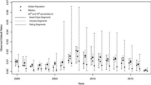
• asset class: SME, Large Corporates, Banks and Financial Companies, Ship Finance, Aircraft Finance, Real Estate Finance, Project Finance, Commodities Finance, Sovereigns, Public Services, Private Banking;

• industry: Agriculture, Hunting and Forestry, Fishing and its Products, Mining, Manufacturing, Utilities, Construction, Wholesale and Retail, Hotels and Restaurants, Transportation and Storage, Communications, Finance and Insurance, Real Estate and Rental and Leasing, Professional, Scientific and Technical Services, Public Administration and Defence, Education, Health and Social Services, Community, Social and Personal Services, Private Sector Services, Extra-territorial Services, and Individual; and

• rating: mapped to S&P rating categories (from AAA to C), as well as defaulted.

In each category, Figure 1 shows the observed default rates of the 25% best and the 25% worst segment, as well as the median (only if there are at least 100 loans in the particular subcategory).

3.3.2. LGD and EAD platform

The LGD platform contains extensive information about defaults on loan level for non-retail exposures including information regarding collateral. The LGD is pre-calculated based on the realised loss per outstanding unit. Slightly different LGD definitions do not affect the results significantly.

The dataset contains over 186,000 defaulted loans after 2000, both resolved (92.5%) and unresolved cases (7.5%). The number of resolved loans between 2000 and 2017 with non-zero exposure is 161,365 from 93,775 different obligors with an average EAD of 3 million Euros. The three most represented asset classes are SME (62.57%), Large Corporates (16.61%), and Real Estate Financing (12.42%). The three most represented industries are Manufacturing (16.44%), Real Estate, Rental, and Leasing (15.94%) and Wholesale and Retail Trade (14.01%).

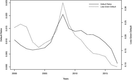
LGD samples outside the $[0,1]$-interval are possible and are not rare for workout LGDs. Typically, the realised workout LGDs in loan level inhibit the bimodal distribution, as also shown in Figure 2 for our dataset. The mean of the realised LGDs (referenced by default year) are highly correlated with the observed default rates as shown by Figure 3. However, some of the defaults in the dataset are not resolved yet, leaving low average realised LGDs in the last five years. A report regarding the LGD distribution of Large Corporate exposures in this dataset (Rainone & Brumma, 2019) and a study about a downturn effect in the LGD pattern (Brumma & Rainone, 2020) were conducted.

Figure 2. Histogram and Boxplot of the realised LGD.

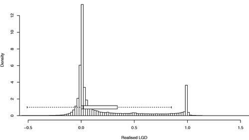
Figure 3. Observed default rates and realised loss given default for each year.

4. Result

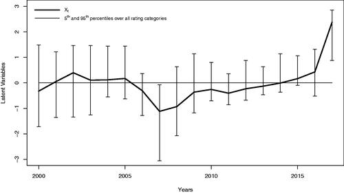
For the observed default rates, the maximum likelihood method gives an estimated $\widehat{p}=27.95\%$ (equivalent to an asset correlation of ${\widehat{p}}^2=7.81\%$). For a comparison, Frye (2000b) reports a p of 23% (for bonds) and Düllmann and Gehde-Trapp (2004) report p to be approximately 20% (for bonds and loans). Under the IRBA, institutions have to apply an asset correlation between 3% and 24% in most cases.

Figure 4 depicts the implied latent variables time-series. During the global financial crisis, which started in 2007, the downturn effect is observed soon after the Lehmann fall in 2008. The implied latent variables in both years are at the lowest points compared to others. In comparison, the implied latent variable in 2017 is high due to the low observed default rate in 2017, as shown in Figure 1.

Figure 4. Estimated latent variables.

4.1. LGD’s systematic sensitivity

To avoid a potential bias originated from cases with an extraordinarily long workout duration, samples with an excessively long workout duration are excluded. About 95% of the resolved defaults in the database have workout durations less than six years, and we choose this to be the cutting point. We successively extend the maximum workout duration length in the analysis to replicate a portfolio of a randomly chosen financial institution. Due to the model design, the results should be interpreted at a portfolio level.

The results presented in Table 1 confirm that the economic conditions during the workout years influence the expected LGD. Thus, an approach using only a single latent variable for the LGD might be inappropriate. Obviously, the sensitivity is highest in the default year and diminishes with increasing default age.

Table 1. LGD’s systematic sensitivity coefficient towards the latent variables from different years during the workout period.

	$q_{t_d}$	$q_{t_d+1}$	$q_{t_d+2}$	$q_{t_d+3}$	$q_{t_d+4}$	$q_{t_d+5}$	${\sigma }_{ϵ}^2$
$T=0$	0.3472						0.0005
$T\le 1$	0.3834	0.0779					0.0012
$T\le 2$	0.3796	0.2745	−0.2418				0.0035
$T\le 3$	0.4093	0.3347	0.0702	−0.1045			0.0065
$T\le 4$	0.4040	0.3288	0.1101	0.0895	−0.1817		0.0080
$T\le 5$	0.4344	0.3188	0.1345	0.0839	−0.0370	0.1934	0.0094

q_t is the sensitivity of expected LGD towards X_t and ${\sigma }_{ϵ}^2$ is the variance of the residuals. T represents the workout duration, so each row can be understood as banks’ limit strategies for workout duration.

4.2. Performance analysis

The results obtained from the previous section suggest that incorporating multiple latent variables from several workout years for a downturn LGD estimation increases the explanatory power. Four basic downturn LGD estimation procedures based on a latent variable approach are chosen for this paper. The idiosyncratic risk will not be evaluated since the focus of the downturn LGD methods is to measure the systematic risk. It is necessary to measure the performance parameters independent from bias correction methods (if any bias in the data exists). Otherwise, it can be argued that the good performance of our method could not only come from the use of a latent variable approach but also from the chosen bias correction. Thus, neither bias correction nor conservatism add-on will be applied.

The performance of the following downturn LGD estimations is compared for the year t (we refer t as today). Up to the time point t, the latent variables are assumed to be available.

(1) A forward-looking single-factor estimation. This procedure assumes that the expected LGD depends only on the (fully-weighted) today’s latent variable, which will be stressed (set to $-{\Phi }^{-1}(0.999)$). (A1) $$\begin{array}{c}\mathbb{E}[LG{D}_i|X_t=-{\Phi }^{-1}(0.999)]=\widehat{\mu }-\widehat{\sigma }(1·X_t+\underset{\text{loan}-\text{specific}\mathrm{ }\text{risk}\mathrm{ }\text{is}\mathrm{ }\text{set}\mathrm{ }\text{to}\mathrm{ }\text{zero}}{\underbrace{0·Z_C}}).\hfill \end{array}$$(A1)

(2) A backward-looking single-factor estimation. This procedure assumes that the expected LGD depends on the (fully-weighted) default year’s latent variable. The latent variable is stressed only, if the default year is t. (A2) $$\begin{array}{c}\mathbb{E}[LG{D}_i|X_{t_d},\mathrm{ }\text{and}\mathrm{ }\text{if}\mathrm{ }t=t_d:X_{t_d}=-{\Phi }^{-1}(0.999)]=\widehat{\mu }-\widehat{\sigma }(1·X_{t_d}+0·Z_C).\hfill \end{array}$$(A2)

(3) A three-years-factors estimation. Compared to the previous methods, this estimation method incorporates multiple latent variables. If the default age is shorter than three years, the last latent variable will be stressed. Otherwise, only the first three realised latent variables after default are included in the estimation (in this particular case, there is no stressed latent variable). This procedure weights the relevant latent variables equally to avoid overfitting. (A3) $$\begin{array}{c}\mathbb{E}[LG{D}_i|X_{t_d},\dots ,X_{t_d+2},\mathrm{ }\text{and}\mathrm{ }\text{if}t\le t_d+2:X_t=-{\Phi }^{-1}(0.999)]\hfill \\ \hfill & =\widehat{\mu }-\widehat{\sigma }(\sum _{s=t_d}^{\min (t_d+2,t)}\underset{\text{equal}\mathrm{ }\text{weight}\mathrm{ }\text{on}\mathrm{ }\text{each}\mathrm{ }\text{workout}\mathrm{ }\text{year}}{\underbrace{\sqrt{\frac{1}{\min (3,t-t_d+1)}}}}·X_s+0·Z_C).\hfill \end{array}$$(A3)

(4) A complete-history based estimation. Different from the last one, this approach incorporates the complete history of past latent variables within the workout duration and stresses only today’s latent variable. All latent variables are equally weighted. (A4) $$\begin{array}{c}\mathbb{E}[LG{D}_i|X_{t_d},\dots ,X_{t-1},\mathrm{ }\text{and}\mathrm{ }{X}_t=-{\Phi }^{-1}(0.999)]\hfill \\ \hfill & =\widehat{\mu }-\widehat{\sigma }(\sum _{s=t_d}^t\underset{\text{equal}\mathrm{ }\text{weight}\mathrm{ }\text{on}\mathrm{ }\text{each}\mathrm{ }\text{workout}\mathrm{ }\text{year}}{\underbrace{\sqrt{\frac{1}{t-t_d+1}}}}·X_s+0·Z_C).\hfill \end{array}$$(A4)

Both parameters $\widehat{\mu }$ and $\widehat{\sigma }$ are estimated by the expected value and the standard deviation of the institutions’ portfolio LGD, which are estimated solely from past information for an out-of-time analysis. In practice, this will be heavily influenced by resolution bias, which generally leads to an underestimation of LGD. Instead of q acquired from the previous result in Table 1, we use equal weights on all of these estimators to avoid overfitting, since the dataset used in the Monte Carlo simulations and for the estimation of q is identical.

It is not difficult to give a first estimate about the degree of conservatism of the four procedures. The number of exposures in a random portfolio which are affected by the stressed latent variable varies in different procedures. A1 is the most conservative estimation procedure (likely to be borderline excessive) since it always includes a stressed component for all exposures, while A2 is the least conservative because it stresses the latent variable only, if the loan defaults in the current year. Both A3 and A4 lie in-between in terms of conservativeness. For instance, if today is 2020 and for a loan, which defaulted in 2017 but is still unresolved, A1 considers only one single stressed component (2020), A2 considers only the 2017s (unstressed) latent variable, A3 considers the 2017–2019s (unstressed) latent variables, and A4 considers the 2017–2019s (unstressed) latent variables and the stressed component (2020).

4.2.1. Comparison to the FIRBA

In this section, we compare the performance of the LGD estimation methods A1-A4 with the LGD methodology under the FIRBA. The FIRBA will become more important, because the recent Basel reforms (Basel Committee on Banking Supervision, 2017) forbid the use of the AIRBA for exposures to some asset classes such as exposures to corporates with consolidated revenues above €500 millions and financial institutions. Under the FIRBA, senior claims on financial institutions and other corporates will be assigned a 45% LGD and a 40% LGD, respectively. The LGD applicable to a collateralised transaction is calculated as the exposure weighted average of the LGD applicable to the unsecured part of an exposure and the LGD applicable to the collateralised part of an exposure.

The relevant asset classes for the FIRBA, which are available in the dataset, are Large Corporates, Banks and Financial Companies, Sovereigns, and Private Banking. Where assumptions are necessary to calculate LGDs under the FIRBA, they are always generous in the sense that the simulation should produce the least amount of waste. For secured loans, the collateral is always treated as eligible and financial collateral’s haircut is assumed to be 0%. Nonetheless, both A3 and A4 produce significantly lower waste than the regulatory downturn LGD under the FIRBA, while maintaining a similar survival chance.

The average of the survival rates is calculated as a geometric mean, while the average of the waste is an arithmetic mean, due to the nature of each parameter. As expected, the FIRBA achieves the 99.9% survival rate on average since it is a very conservative approach. However, even under generous assumptions, Table 2 confirms that the LGD based on the FIRBA is wasteful compared to other methods. In fact, its performance is similar to A1 on average, both the survival chance and the waste. However, A1 is adapting to the economic situation as more information becomes available. Its waste values are higher than the FIRBA’s waste only during 2005–2008. If more data becomes available, a more accurate estimation by A1 may be achievable compared to the FIRBA. In summary, the downturn LGD is overestimated by about 22% under the FIRBA, whereas methods A3 and A4 result in an overestimation of approximately 13% and 16%, respectively, while maintaining at the same time a high survivability of 99.9%.

Table 2. Comparison of survival chance and waste of different downturn LGD estimation models with the FIRBA for relevant asset classes in % for each year from 2005 until 2017.

		Survival chance
	$\widehat{\mu }$	(Waste)
	($\widehat{\sigma })$	A1	A2	A3	A4	FIRBA
2005	21.23	100	100	100	100	100
	(7.66)	(23.80)	(5.02)	(10.49)	(14.55)	(22.10)
2006	20.24	100	100	100	100	100
	(8.23)	(25.90)	(4.01)	(7.83)	(14.04)	(18.92)
2007	19.68	100	100	100	100	100
	(8.66)	(34.14)	(14.87)	(23.58)	(26.55)	(31.08)
2008	17.96	100	100	100	100	100
	(9.54)	(26.30)	(15.24)	(21.89)	(24.67)	(23.34)
2009	19.09	100	100	100	100	100
	(7.79)	(21.39)	(12.76)	(19.59)	(21.12)	(23.39)
2010	20.01	100	100	100	100	100
	(6.96)	(19.76)	(6.24)	(15.84)	(17.03)	(22.02)
2011	20.76	100	100	100	100	100
	(6.60)	(22.47)	(9.45)	(17.07)	(18.94)	(25.52)
2012	20.13	100	100	100	100	100
	(7.07)	(17.82)	(4.12)	(10.99)	(14.21)	(19.90)
2013	20.61	100	100	100	100	100
	(6.40)	(18.83)	(6.42)	(12.25)	(15.12)	(21.78)
2014	20.21	100	92.64	100	100	100
	(7.08)	(17.13)	(1.55)	(8.21)	(11.74)	(18.02)
2015	20.68	100	0.27	99.26	100	100
	(6.36)	(12.60)	(0.27)	(2.39)	(6.31)	(13.74)
2016	20.68	100	2.96	99.63	100	100
	(6.22)	(12.44)	(0.34)	(2.43)	(5.66)	(14.87)
2017	20.81	100	100	100	100	100
	(6.15)	(22.96)	(5.90)	(13.01)	(14.65)	(27.70)
Average		100	48.11	99.91	100	100
		(21.19)	(6.63)	(12.74)	(15.74)	(21.72)

$\widehat{\mu }\mathrm{ }\text{and}\mathrm{ }\widehat{\sigma }$ are the estimated portfolio’s realised LGD mean and standard deviation based on historical data up to each year. A1 is the forward-looking single-factor estimation, A2 is the backward-looking single-factor estimation, A3 is the three-years-factor estimation, A4 is the complete-history based estimation, and FIRBA is the LGD assigned according to the FIRBA.

4.2.2. Comparison to the AIRBA

Similarly to the previous simulation, we compare our proposed methods with the AIRBA. According to the Basel Committee on Banking Supervision (2017), supervisors may permit the use of the AIRBA to the corporate asset class with a consolidated revenue of less than €500 millions. In our dataset, the relevant asset class would be exposures to SMEs.

Although the EBA has spent a lot of efforts to harmonise the calculation of capital requirements under the AIRBA (EBA, 2019), institutions still have some leeway in determining own downturn LGD estimates. Choosing a specific downturn LGD estimation method appropriate for the AIRBA may reduce the representativeness of our analysis. Therefore, we choose three methods that are eligible under the EBA guideline and represent different level of conservatism: (AIRBA-L) $$\mathit{DLG}{D}_L:=\frac{LG{D}_{\text{max},t}+LG{D}_{{\text{max}}_2,t}}{2},$$(AIRBA-L) (AIRBA-M) $$\mathit{DLG}{D}_M:=LG{D}_{\text{max},t},$$(AIRBA-M) (AIRBA-H) $$\mathit{DLG}{D}_H:=\min (105\%,\frac{\sum _{s\le t}LG{D}_{s,t}}{\left|\right\{s|s\le t\}|}+15\%),$$(AIRBA-H) where $LG{D}_{\text{max},t}$ denotes the maximum, $LG{D}_{{\text{max}}_2,t}$ the second maximum observed LGD until t, and $LG{D}_{s,t}$ the observed average LGD of facilities defaulted in s and resolved in t. Assuming downturn periods are associated with high LGDs, the $LG{D}_{\text{max},t}$ should be a good proxy of the worst downturn year. Obviously, DLGD_L yields the lowest downturn LGD and DLGD_H is the most conservative method, which is introduced as a backstop for the case the two other methods cannot be applied.

The simulation will be done with the application of the LGD input floors, as introduced by the Basel Committee on Banking Supervision (2017), and without them. Input floors are 25% for unsecured exposures and vary between 0% and 15% depending on the type of collateral.

The results shown in Table 3 are very concerning. Briefly summarised, the downturn LGD methods as proposed by the EBA (AIRBA-L and AIRBA-M) are inadequate to ensure the 99.9% survival chance. Most of the failures happen in the post-crisis period. Most likely, banks will identify 2008/2009 as the downturn periods in compliance with the proposed regulatory technical standard (EBA, 2018). Even though institutions are required for thorough impact assessment in compliance to the proposed guideline (EBA, 2019), the information on the downturn impact associated with the financial crisis is simply not available in 2010 yet. This is due to the fact that the workout duration can exceed two years. The impacts observed from the past are unfortunately still inadequate. Even the AIRBA-M estimate only shows a survival rate of 80.9% without input floors mostly due to failures during post-crisis periods.

Table 3. Comparison of survival chance and waste of different downturn LGD estimation models with the AIRBA for SME asset class in % for each year from 2005 until 2017.

		Survival chance
	$\widehat{\mu }$	(Waste)
	($\widehat{\sigma })$	A1	A2	A3	A4	AIRBA-L	AIRBA-M	AIRBA-H
2005	14.54	100	99.80	100	100	90.98	93.43	100
	(3.60)	(9.60)	(2.72)	(5.52)	(6.49)	(1.36)	(1.47)	(13.48)
2006	15.33	100	86.66	100	100	89.78	92.20	100
	(3.18)	(7.79)	(1.31)	(3.90)	(4.77)	(1.37)	(1.48)	(12.97)
2007	16.14	100	73.21	99.99	100	84.13	89.02	100
	(2.94)	(6.81)	(1.09)	(3.94)	(4.64)	(1.27)	(1.42)	(12.71)
2008	16.62	100	100	100	100	99.21	99.33	100
	(4.02)	(10.69)	(4.02)	(8.81)	(10.06)	(2.27)	(2.34)	(13.26)
2009	16.86	100	99.99	100	100	86.78	88.17	100
	(3.43)	(8.00)	(4.00)	(7.31)	(7.99)	(1.47)	(1.54)	(12.41)
2010	17.27	100	64.81	99.98	100	62.01	62.68	100
	(2.86)	(5.70)	(1.12)	(4.06)	(4.74)	(1.07)	(1.08)	(11.85)
2011	17.56	100	16.23	99.12	99.97	13.52	15.23	100
	(3.66)	(6.14)	(0.66)	(3.15)	(4.20)	(0.62)	(0.64)	(9.82)
2012	18.36	100	42.08	99.11	100	70.72	98.57	100
	(3.73)	(7.09)	(0.96)	(3.22)	(5.14)	(1.33)	(2.90)	(10.57)
2013	18.48	100	65.08	99.99	100	93.26	100	100
	(4.86)	(10.67)	(1.33)	(4.95)	(7.60)	(2.25)	(5.10)	(10.65)
2014	18.61	100	1.52	85.86	99.99	59.83	99.78	100
	(5.15)	(8.79)	(0.49)	(1.86)	(4.63)	(1.24)	(3.70)	(7.88)
2015	18.79	100	6.39	93.05	100	97.75	100	100
	(5.37)	(10.43)	(0.57)	(2.16)	(5.29)	(2.63)	(5.53)	(8.83)
2016	18.69	100	1.78	98.81	100	99.94	100	100
	(5.82)	(11.80)	(0.38)	(2.50)	(5.31)	(3.31)	(6.22)	(8.82)
2017	18.47	100	0	33.36	99.60	99.88	100	100
	(6.01)	(11.23)	(−)	(0.57)	(2.25)	(2.63)	(5.54)	(7.65)
Average		100	31.63	90.12	99.97	73.75	80.85	100
		(8.83)	(1.56)	(4.00)	(5.62)	(1.76)	(3.00)	(10.84)
Average						94.62	99.40	100
with input floors						(4.12)	(5.25)	(10.84)

$\widehat{\mu }\mathrm{ }\text{and}\mathrm{ }\widehat{\sigma }$ are the estimated portfolio’s realised LGD mean and standard deviation based on historical data up to each year. A1 is the forward-looking single-factor estimation, A2 is the backward-looking single-factor estimation, A3 is the three-years-factor estimation, A4 is the complete-history based estimation, AIRBA-L is the downturn LGD calculated according to the AIRBA with a low level of conservatism, AIRBA-M with a medium level of conservatism, and AIRBA-H with a high level of conservatism.

The inclusion of input floors brings the survival chance to 99.4%. On the one hand, this is a reassurance that input floors help approaching the 99.9% survivability, assuming banks will at least adopt an (M)-type estimate. On the other hand, they should be understood as a makeshift solution and do not really solve the conceptual drawbacks of a macroeconomic based downturn LGD estimation. Moreover, input floors generally give the wrong incentive for low-risk banks to increase their risks, since they are not risk sensitive.

In comparison, method A4 gives a stunning precision towards the required 99.9% survivability, without any input floors. As expected, the LGD calculated under AIRBA-H is sufficiently conservative as well, but with a 10% LGD overestimation compared to a 5% waste from A4.

While the results presented in Tables 2 and 3 are calculated under the assumption of a large diversified loan portfolio with negligible idiosyncratic risk, our calculations show that the results also hold for smaller default portfolios (see Table 4).

Table 4. Average survival chance and average waste in % when only $n$ default cases are resolved per year.

	Average survival chance
	(Average waste)
	A3	A4	A3	A4	FIRBA	A3	A4	AIRBA-L	AIRBA-M	AIRBA-H
$n$	(I)		(II)			(III)
100	88.40	96.34	94.57	98.73	99.99	78.70	89.83	79.98	88.38	99.02
	(7.19)	(8.72)	(13.09)	(15.84)	(21.72)	(5.30)	(6.39)	(5.36)	(6.09)	(10.95)
200	92.32	98.88	96.51	99.71	100	83.81	95.45	85.21	93.78	99.91
	(6.77)	(8.50)	(12.91)	(15.77)	(21.73)	(4.63)	(5.89)	(4.73)	(5.58)	(10.86)
300	93.70	99.54	97.48	99.92	100	86.42	97.58	88.17	96.07	99.98
	(6.63)	(8.44)	(12.82)	(15.73)	(21.72)	(4.37)	(5.75)	(4.49)	(5.43)	(10.85)
400	94.65	99.77	98.21	99.99	100	87.72	98.65	90.11	97.21	100
	(6.56)	(8.42)	(12.79)	(15.73)	(21.71)	(4.24)	(5.68)	(4.35)	(5.35)	(10.84)
500	95.43	99.90	98.77	99.99	100	88.79	99.15	91.29	97.96	100
	(6.52)	(8.42)	(12.77)	(15.74)	(21.72)	(4.15)	(5.65)	(4.27)	(5.31)	(10.84)
	⋮	⋮	⋮	⋮	⋮	⋮	⋮	⋮	⋮	⋮
1000	97.08	100	99.91	100	100	90.12	99.97	94.62	99.40	100
	(6.44)	(8.41)	(12.74)	(15.74)	(21.72)	(4.00)	(5.62)	(4.12)	(5.25)	(10.84)

A3 is the three-years-factor estimation, A4 is the complete-history based estimation, FIRBA is the LGD assigned according to the FIRBA, AIRBA-L is the downturn LGD calculated according to the AIRBA with a low level of conservatism and LGD input floors, AIRBA-M with a medium level of conservatism and LGD input floors, and AIRBA-H with a high level of conservatism and LGD input floors. (I) is calculated in the global population, (II) only for relevant asset classes in the FIRBA, and (III) only for SME asset class.

4.3. Regulatory application

The latent variable approach can be used to improve banking regulation as well as banks’ internal risk management. As the regulatory given LGD values under the FIRBA are not based on a rigorous econometric approach, our results can serve the regulatory authorities as a benchmark indicating whether these LGD values are adequately conservative or overly burdensome. The latent variable approach requires as input the long-run average LGD $\widehat{\mu }$ at the portfolio level, its associated standard deviation $\widehat{\sigma },$ the default year t_d, the current year t, and the latent variables of all relevant years $(X_{t_d},\dots ,X_t).$ These parameters can be estimated from the data banks are obliged to provide to regulatory authorities, while the latent variables can be estimated from default rates from a given system, independent from banks.

The results presented in Table 3 suggest that downturn LGDs following the EBA guidelines fail the 99.9% criterion. Therefore, the macroeconomic approach, adopted by the EBA, should be complemented by a latent variable approach based on method A4 as a kind of backstop. Regulatory authorities should provide banks with the input parameters relevant for the latent components, since they represent the overall economic condition. To allow for some degree of model flexibility, institutions should be allowed to estimate their own idiosyncratic factor. The result of the performance test is independent of the idiosyncratic factor model banks want to adopt.

5. Conclusion and discussion

A recently published guideline (EBA, 2019) specifies a macroeconomic approach to estimate downturn LGDs. This approach introduces a methodological mismatch in the downturn definitions and will potentially result in an underestimation of capital requirements. A latent variable approach provides a remedy against these weaknesses. This approach is able to estimate downturn LGDs at a 99.9% confidence level, whereas a macroeconomic approach with a medium level of conservatism achieves only a confidence level of 99.4%, only if an input floor is imposed. Input floors however, cannot remedy the conceptual flaws of the macroeconomic downturn approach and induce disincentives. A confidence level of 99.9% can be reached, if the downturn LGD is determined using an overly conservative macroeconomic approach, e. g. the backstop method introduced in the guideline. But, this method induces a significantly higher level of capital compared to the latent variable approach. This in turn, reduces a bank’s lending capacity and leads to higher borrowing costs. A latent variable approach is efficient in the sense that it ensures a given level of safeness, i.e., a confidence level of 99,9%, with lower capital requirements than any other method proposed in the aforementioned guideline. By using a time series of latent variables rather than a single latent variable, a latent variable approach can be applied to estimate market based LGDs for defaulted exposures with a short workout period as well as workout LGDs for defaulted exposures with a long workout period.

In spite of its strengths the latent variable approach has a major drawback that may impede its use in regulatory requirements and in banks’ risk management. The concept of a latent variable is less intuitive than a macroeconomic approach and may be considered as a kind of black box. Due to this reason, we recommend to complement rather than to substitute the macroeconomic approach by a latent variable approach proposed in this paper.

Disclosure statement

No potential conflict of interest was reported by the authors.

Notes

1 GCD is a non-profit association owned by its member banks from around the world and active in data-pooling for historical credit data. As of 2020, it has 55 members across Europe, Africa, North America, Asia, and Australia. For details: https://www.globalcreditdata.org

2 Counted in loan-years. Assuming the typical duration to maturity or default time is similar throughout the segments, the composition remains unchanged when counted in number of loans.

References

- Bade, B., Rösch, D., & Scheule, H. (2011). Default and recovery risk dependencies in a simple credit risk model. European Financial Management, 17(1), 120–144. Retrieved from https://doi.org/10.1111/j.1468-036X.2010.00582.x
- Barco, M. (2007). Going downturn. Risk, 20(8), 70–75.
- Basel Committee on Banking Supervision. (2017). Basel III: finalising post-crisis reforms.
- Betz, J., Kellner, R., & Rösch, D. (2018). Systematic effects among loss given defaults and their implications on downturn estimation. European Journal of Operational Research, 271(3), 1113–1144. Retrieved from https://doi.org/10.1016/j.ejor.2018.05.059
- Brumma, N., & Rainone, N. (2020). Downturn LGD study 2020. Global Credit Data.
- Cosimano, T., & Hakura, D. (2011). Bank behavior in response to Basel III: A cross-country analysis. IMF Working Papers, 11(119), 1. Retrieved from https://doi.org/10.5089/9781455262427.001
- Düllmann, K., & Gehde-Trapp, M. (2004). Systematic risk in recovery rates: an empirical analysis of US corporate credit exposures. Deutsche Bundesbank, Discussion Paper Series 2: Banking and Financial Supervision.
- European Banking Authority (EBA). (2018). Final Draft Regulatory Technical Standards: On the specification of the nature, severity and duration of an economic downturn in accordance with Articles 181(3)(a) and 182(4)(a) of Regulation (EU) No 575/2013.
- European Banking Authority (EBA). (2019). Final Report: guidelines for the estimation of LGD appropriate for an economic downturn (‘Downturn LGD estimation’).
- Frye, J. (2000a). Collateral damage: A source of systematic credit risk. Risk, 13(4), 91–94.
- Frye, J. (2000b). Depressing recoveries. Risk, 13(11), 106–111.
- Frye, J. (2013). Loss given default as a function of the default rate. Federal Reserve Bank of Chicago.
- Frye, J., & Jacobs Jr, M. (2012). Credit loss and systematic loss given default. Journal of Credit Risk, 8(1), 1–32. Retrieved from https://doi.org/10.1142/9789814417501_0011
- Giese, G. (2005). The impact of PD/LGD correlations on credit risk capital. Risk, 18(4), 79–84.
- Gordy, M., & Heitfield, E. (2002). Estimating default correlations from short panels of credit rating performance data. [Working paper].
- Hillebrand, M. (2006). Modeling and estimating dependent loss given default. Risk, 19(9), 120–125.
- Koopman, S. J., Lucas, A., & Schwaab, B. (2011). Modeling frailty-correlated defaults using many macroeconomic covariates. Journal of Econometrics, 162(2), 312–325. Retrieved from https://doi.org/10.1016/j.jeconom.2011.02.003
- Mikkelsen, J. G., & Pedersen, J. (2017). A cost-benefit analysis of capital requirements for the Danish economy. Danmarks Nationalbank: Working Paper, 123.
- Miles, D., Yang, J., & Marcheggiano, G. (2013). Optimal bank capital. The Economic Journal, 123(567), 1–37. Retrieved from https://doi.org/10.1111/j.1468-0297.2012.02521.x
- Pykhtin, M. (2003). Unexpected recovery risk. Risk, 16(8), 74–79.
- Pykhtin, M. (2004). Multi-factor adjustment. Risk, 17(3), 85–90.
- Pykhtin, M., & Dev, A. (2002). Analytical approach to credit risk modelling. Risk, 15(3), S26–S32.
- Rainone, N., & Brumma, N. (2019). LGD report 2019 – Large corporate borrowers. Global Credit Data.
- Schönbucher, P. (2001). Factor models: Portfolio credit risks when defaults are correlated. The Journal of Risk Finance, 3(1), 45–56. Retrieved from https://doi.org/10.1108/eb043482
- Tasche, D. (2004). The single risk factor approach to capital charges in case of correlated loss given default rates. [Working Paper].
- Thakkar, D., & Crecel, R. (2019). PD benchmarking report 2019. Global Credit Data.
- Van den Heuvel, S. J. (2008). The welfare cost of bank capital requirements. Journal of Monetary Economics, 55(2), 298–320. Retrieved from https://doi.org/10.1016/j.jmoneco.2007.12.001