Outpatient clinic scheduling with limited waiting area capacity

Abstract

This paper proposes an iterative simulation optimisation approach to maximise the number of in-person consultations in the blueprint schedule of a clinic facing same-day multi-appointment patient trajectories and restrictions on the number of patients simultaneously allowed in the waiting area, taking into account the combined effects of early arrival times (patients arriving early from home), bridging times (minimum time required between appointments) and waiting times (due to randomness in patient arrivals and provider punctuality). Our approach combines an Integer Linear Program (ILP) that maximises the number of in-person consultations considering the effect of average early arrival and bridging times and a Monte Carlo simulation (MCS) model to include the effect of waiting times due to randomness. We iteratively adapt our parameters in the ILP until the MCS model returns a 95% confidence interval of the number of patients in the waiting area that does not exceed its capacity. Our results reveal the impact of early arrival, bridging and waiting times on the number of in-person appointments that may be included in a blueprint schedule. Our results further show that careful design of the blueprint schedule allows our case study clinics to organise a vast majority of their appointments in-person.

Keywords:

• Health services
• mathematical programming
• scheduling
• simulation
• optimisation

1. Introduction

Distancing measures due to the COVID-19 pandemic, requiring patients to stay, e.g. 1.5 meters apart, impose a limit on the number of patients that can be simultaneously present in a shared space such as hospital waiting areas. To avoid crowded waiting areas the starting times of in-person consultations must be separated in time, possibly reducing the number of in-person consultations, replacing consultations by telephone or video calls, or extending consultation hours. The pressure on available space is even more severe due to patients on same-day multi-appointment trajectories, as such patients must bridge the time between subsequent appointments and may occupy the waiting area for a considerable amount of time. As the number of available medical professionals is a serious limiting factor in healthcare delivery, even more so during the COVID-19 pandemic, and, often, in-person consultations are preferred over telephone or video consultations, efficient scheduling of consultations is of utmost importance to maximise the number of consultations that can be realised taking into account the limited availability of space. This paper proposes a model to optimise the number of consultations that can take place in-person in the hospital, taking into account same-day multi-appointment patient trajectories and the restrictions imposed on the number of patients simultaneously allowed in the waiting area. To this end, we optimise the hospital’s blueprint schedule (also called appointment schedule, template, or raster), which specifies per time slot and type of resource what patient type should be assigned by the planners.

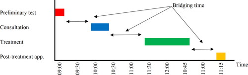
The general setting, we consider is that a patient’s trajectory or visit to the hospital consists of a single appointment or a number of consecutive appointments or stages to be completed on the same day. In a multi-appointment trajectory, the patient might for example first need preliminary testing, such as a blood test or a radiology examination. After this diagnostic test, the patient has a consultation at the outpatient clinic, followed by a second consultation with another physician, or for example by some type of treatment, such as a chemotherapy infusion in case of an oncology clinic or a visit to the plaster room in an orthopaedics department, see Figure 1 for a patient trajectory of four stages: ‘preliminary tests’, ‘consultation’, ‘treatment’ and ‘post-treatment appointment’. We will refer to the time between two consecutive appointments, for example the time between preliminary tests and the consultation and the time between the consultation and the treatment, as bridging time. Typically, a minimum duration applies for these bridging times, for example to cover the time to analyse the blood draw in the laboratory, to analyse test results by radiologists, or to prepare patient specific chemotherapy drugs in the pharmacy. Only after the testing results or drugs are available, the next appointment can take place. This means, for example, that if an oncology patient finishes preliminary tests at 9:15AM and the minimal bridging time equals 45 min, this patient’s consultation cannot start before 10AM. Similarly, if the consultation of this patient starts at 10AM and finishes at 10:30AM and preparation of chemotherapy drugs in the pharmacy takes one hour, the treatment cannot start before 11:30AM, i.e. a bridging time of an hour is minimally required between consultation and treatment. In addition to these bridging times, a preliminary data analysis in our case study clinics revealed that in times of COVID-19, patients who start their visit at the hospital with a consultation or treatment arrive to the waiting area on average 30 min before the planned start of their first consultation or treatment, referred to as early arrival time. Besides early arrival and bridging times, patients also experience waiting times before their scheduled appointments that occur as a consequence of randomness in arrival, consultation and treatment times. The approach proposed in this paper takes into account the combined effects of early arrival, bridging and waiting times in the design of an optimal appointment system.

Figure 1. Schematic depiction of a patient trajectory and timeline.

The physical location of patients during their early arrival, waiting and bridging times depends on the lay-out of the hospital. We assume a patient spends its early arrival, waiting and bridging time before an appointment in the waiting area of that appointment. Thus, during the bridging time between a preliminary test and consultation at the outpatient clinic, the patient is physically present in the waiting area of the outpatient clinic. Note that the waiting areas are typically not fully dedicated to a single consultation or treatment, but are shared over various specialties, e.g. multiple consultation types share the same waiting area, or shared in a carousel, e.g. (part of) the patient’s trajectory shares the same waiting area. Hospitals typically face a complicated case-mix with occupancy of waiting areas determined by a wide variety of patient types with different trajectories. At the time of the design of a blueprint schedule, the actual patients to be treated have not yet been revealed, but the statistical information on historical arrivals is available in the Hospital Information System. Pre-COVID-19 blueprint design approaches did not consider waiting area congestion as a limitation and restriction to the appointment system design, but typically focused on minimising patient waiting time, resource idle time, and overtime. However, under the restrictions due to COVID-19 on the capacity of waiting areas, when creating a blueprint schedule, we now have to take into account the minimum bridging times, as well as the maximum number of patients allowed in the waiting areas. In this paper, we develop an iterative simulation optimisation approach to maximise the number of consultations that can take place in the hospital, taking into account the minimum bridging times between every stage as well as the maximum number of patients allowed in the waiting area of each stage.

Our iterative simulation optimisation approach is designed as follows. First, using an Integer Linear Program (ILP) formulation we determine a deterministic blueprint schedule that maximises the number of in-person consultations taking into account the effect of early arrival and bridging times and the waiting area capacity restrictions. Second, we analyse the effects of waiting times due to randomness in patient arrivals and provider punctuality using a Monte Carlo simulation (MCS) model. Typically, the number of patients in the waiting area increases due to randomness, which may render a schedule that is feasible in the deterministic setting of the ILP infeasible under randomness. If the MCS model shows that occupancy of the waiting area exceeds the capacity of the waiting area, then based on the outcomes of the MCS model, the input parameters on waiting area capacity and number of appointments per appointment type in the ILP are adapted, the ILP is solved again and the resulting blueprint schedules are evaluated using the MCS model. We iteratively adapt our parameters and evaluate the blueprint schedules, until a solution is found for which the MCS model shows that the 90% confidence interval of the number of patients present in the waiting area does not exceed the waiting area capacity. The final ILP schedule is then used as blueprint schedule.

This research is inspired by requests from multiple hospitals in The Netherlands to help maintain patient volumes and help design appointment systems for non-COVID-19 related care. During the first COVID-19 wave, patient volumes in The Netherlands were drastically reduced for non-emergent care to almost zero. Up-scaling of outpatient clinic appointments was subsequently done primarily based on intuition and typically in a conservative way to safeguard patient safety. This led to inefficient use of capacities and typically empty waiting areas, except for clinics with high bridging times. Hospital staff identified a need for an appointment system that maximises the amount of possible in-person consultations and continuation of treatments in such a way that these hospital visits are safe for patients and staff. In this paper we consider two case studies: a rheumatology clinic and a medical oncology & haematology clinic. Sint Maartenskliniek (SMK) is a specialised hospital for orthopaedic surgery, rheumatology, and rehabilitation medicine. The rheumatology clinic of SMK serves 225 patients per working day on average. Patients typically follow a standardised trajectory. First patients take a blood test, followed by a consultation and tests with a nurse. Following a bridging time to analyse the results of the blood test, the patient has a consultation with a rheumatologist. Afterwards, some patients may need to have a blood test or radiology examination or visit the pharmacy to collect medication. Bridging times in the rheumatology clinic are typically between fifteen minutes and half an hour. Every patient who has to bridge time does this in a shared waiting area. University Medical Center Utrecht (UMCU) is a large academic hospital in The Netherlands. The medical oncology & haematology clinic of UMCU serves 194 patients per working day on average, with a shared waiting area, as well as chemotherapy, immunotherapy, and other drug therapies with an individual waiting area. A blood draw might be required for patients visiting the oncology clinic before their consultation or treatment, to ensure the patient is viable for obtaining the treatment. Bridging times in the oncology clinic are typically one hour or more, as blood draws need to be analysed before the consultation, and drugs need to be prepared on an individual basis for patients after the consultation. Due to the nature of the treatments, treatment times can take up to 8 h, restricting the possibilities for the appointment template design.

The contribution of our paper is twofold. First, we develop an iterative simulation optimisation approach, consisting of an ILP model and a MCS model, that optimises the blueprint schedule for a hospital, taking into account multi-appointment patient trajectories. The main assumption that makes our ILP model tractable is that early arrival times and appointment durations are deterministic. Although this assumption is common for the development of blueprint schedules, this assumption is clearly not realistic in practice. We therefore developed our MCS model to investigate the quality of the ILP schedule under randomness in early arrival times and appointment durations. Our iterative approach allows for inclusion of the effects of these random durations in the ILP blueprint schedule. Although blueprint optimisation in general is widely considered in literature, including the waiting room occupancy as the main restriction is not yet considered. Due to distancing measures induced by the COVID-19 pandemic, including this metric in blueprint optimisation, as proposed in this paper, became very relevant. Second, we show through our case studies that our approach is very generic and can be applied to outpatient clinics with various characteristics.

The remainder of this paper is organised as follows. Section 2 provides an overview of the literature on waiting area congestion and appointment planning under COVID-19. Section 3 introduces our model and simulation optimisation approach for the blueprint design of same-day multi-appointment systems, followed by our case study results in Section 4. Section 5 concludes with a summary of the main findings, discussions, and opportunities for future research directions.

2. Literature

Healthcare is under severe pressure from the COVID-19 pandemic, which is manifested in several ways: cancellations of elective treatments (COVIDSurg Collaborative, 2020; van Giessen et al., 2020); stress experienced by healthcare professionals (da Silva & Barbosa, 2021; González-Gil et al., 2021); reallocation of medical resources and staff to COVID-19 activities (Emanuel et al., 2020) and (the threat of) overcrowded ICU and wards due to a sudden increase in the number of infected patients (RIVM, 2020). Besides modelling disease spreading, e.g. (Wu et al., 2020), mathematical models may support decision making to allocate scarce resources, see (Currie et al., 2020), to help minimising the impact of COVID-19 related care and measures on non-COVID-19 patients. Outpatient clinics and day-treatment facilities are not affected by bed shortage at ICU or ward. However, these clinics are considerably affected by distancing measures as they typically include a waiting area with limited capacity, which restricts the number of patients simultaneously present (Zonderland, 2021). Replacing in-person appointments by digital ones might allow continuation the majority of appointments, however, this replacement is not always possible and is not preferred by patients and physicians (Wehrle et al., 2021). To support continuation of in-person care for a large share of non-COVID-19 patients, it is therefore of utmost importance to use the capacity of outpatient clinics at its maximum, which calls for appointment scheduling under restrictions on the capacity of the waiting area.

Appointment planning and scheduling is widely studied in healthcare (Ahmadi-Javid et al., 2017; Leeftink et al., 2018; Marynissen & Demeulemeester, 2019; Zonderland & Boucherie, 2021). However, the challenges incurred by the COVID-19 pandemic complicate the appointment planning practices, through constraining the use of waiting areas. Therefore, in the remainder of this section we will discuss relevant literature on outpatient clinic appointment planning with waiting room restrictions. We also include relevant literature focused on single-day multi-appointment settings, where bridging time between appointments results in increased pressure on waiting area congestion.

Multi-appointment scheduling focuses on performance measures from the perspective of the patient (e.g. waiting time), provider (e.g. overtime), and system (e.g. utilisation), or a combination thereof (Lamé et al., 2016). One-stop-shops and treatment carousels are examples of such same-day multi-appointment scheduling problems. The common approach in design of appointment systems is via blueprint schedules obtained via an Integer Linear Programming (ILP) approach (Leeftink et al., 2018; Marynissen & Demeulemeester, 2019). Such schedules typically assume ample capacity of the waiting area, and therefore do not include occupancy of the waiting area, that introduces a considerable restriction on the appointment schedule under COVID-19 distancing measures.

Outpatient clinics or day-treatment facilities with limited waiting area need to take waiting room congestion into account in their appointment system design, which might cause typically well performing appointment rules, such as the Dome rule (Yang & Cayirli, 2020), to be unsuitable for appointment planning. Waiting room congestion in appointment scheduling is primarily attributed to poor schedule execution and poor patient punctuality (Cox & Boyd, 2018). Congestion in the waiting area is known to affect patient and provider satisfaction. To mitigate amongst others these congestion effects, Lin et al. (2017) minimised the combination of waiting time, overtime and waiting area congestion by evaluating various appointment scheduling heuristics and strategies for resource allocation and appointment scheduling. The common approach to take randomness, due to the variability in the rate of referral and patient and provider punctuality, into account in appointment scheduling, is via queueing theory and Monte Carlo simulation (MCS) (Hulshof et al., 2012; Zonderland et al., 2021). (Kortbeek et al., 2017) consider a same-day multi-appointment setting and first use ILP to determine a blueprint schedule and subsequently use queueing theory and MCS to evaluate access times for children with neuromuscular diseases at the Academic Medical Center, Amsterdam. Same day waiting times are studied for an integrated emergency post in (Mes et al., 2021) via MCS, where focus is on evaluation of waiting times as a consequence of randomness in patient arrivals, but waiting area capacity restrictions are not included. A further example that illustrates that performance indicators do not take into account limited waiting area capacity is provided in (Dobish, 2003), that considers oncology clinic planning, a typical example of a multi-appointment planning situation where significant bridging times are required, due to the one-stop-shop setup requiring blood analysis and drug preparation time. In this context, it is empirically shown that same-day multi-appointment schedules have a significant effect on waiting times, compared to a next-day chemotherapy schedule. Although waiting times, patient flow, and provider workload are often included in literature, sharing of a limited waiting area over various specialties or stages in a patient trajectory is not included, leaving the impact of capacity sharing in a finite waiting room an open research direction.

Liang et al. (2015) developed a mathematical program to generate blueprints with a balanced workload for the practitioners in an oncology clinic, and evaluated the effect of the resulting blueprints using discrete event simulation. Given that practitioners are considered resources, just as waiting area space can be defined as a resource, this approach comes most close to our proposed method. However, where providers and treatment locations are related to scheduled appointments with fixed durations, waiting area usage is not scheduled with a fixed duration, as it depends on the appointment schedule. Furthermore, the waiting area is regularly a shared resource by multiple providers (e.g. multiple departments), which requires the joint optimisation of the appointment schedules of these providers in order to ensure the most efficient use of the restricted waiting space. These two aspects complicate the use of available methods in the literature, and are the motivator of our research. Bridging time in multi-appointment scheduling problems occurs when combination appointments or a series of appointments are scheduled on the same day, and patients have to wait between the subsequent appointments. Besides poor schedule execution and patient unpunctuality, we hypothesise that in same-day multi-appointment settings, the schedule design has a significant influence on waiting room congestion as well, due to bridging times. Therefore, research is needed to minimise the waiting room congestion in multi-appointment settings, to comply with the COVID-19 distance measures.

In the remainder of this paper, we will address the design of blueprint appointment schedules for same-day multi-disciplinary, multi-appointment settings with limited capacity in shared and dedicated waiting areas, using a simulation optimisation approach, that combines mathematical modelling and simulation modelling.

3. Model and simulation optimisation approach

This section presents our solution approach for developing a blueprint schedule that maximises the number of in-person consultations that can take place in a hospital taking into account the early arrival times, bridging times between stages and waiting times as well as the maximum number of patients allowed in the waiting area. Our iterative approach for developing the blueprint schedule is outlined in Section 3.1. We continue by introducing the notation in Section 3.2. Then, we present the Integer Linear Program problem formulation for the deterministic blueprint schedule design in Section 3.3. The Monte Carlo simulation model for evaluating the effects of randomness in the patients’ arrival times and the consultation and treatment times is discussed in Section 3.4.

To develop a generically applicable model, we consider a clinic with multiple stages, each stage corresponding to a set of possible appointment types. In accordance with the set up in our case study clinics, the first and last stage are designed as a walk-in system. The intermediate stages are designed as appointment based systems. For these intermediate stages, our aim is to design a blueprint schedule. Patient trajectories may consist of different subsets of the stages and may also consist of a single stage. Note that between stages minimum bridging times may be defined. As an example, patients might need to bridge time between their scheduled consultation or treatment appointment of Stage 3 and a final walk-in visit to the pharmacy in Stage 4, as they have to wait 15 min before going to the pharmacy due to drug preparation or information processing time.

3.1. Iterative simulation optimisation approach

To include waiting area capacity restrictions in blueprint schedule design, we first determine a deterministic blueprint schedule that takes into account the effect of early arrival and bridging times on waiting area capacity using an Integer Linear Program (ILP). As our literature study showed that waiting area occupancy in appointment scheduling is also attributed to poor schedule execution and patient punctuality, we use a Monte Carlo simulation (MCS) model to evaluate the effect of patient and provider punctuality on the performance of the blueprints resulting from the developed ILP. Based on the outcomes of the MCS, the input parameters on waiting area capacity and number of appointments per appointment type in the ILP are adapted, the ILP is solved again, and the resulting blueprint schedules are evaluated using the MCS. We iteratively adapt our parameters and evaluate the blueprint schedules, until a solution is found for which the MCS shows that the 95% confidence interval of the number of patients present in the waiting area does not exceed the waiting area capacity.

Parameter updating of our iterative approach has two elements: (1) the waiting area capacity, and (2) the number of appointments of each appointment type that may be scheduled in the blueprint schedule. In the first run of the ILP, the waiting area capacity parameter is set to the maximum available waiting area capacity of the considered instance and the ILP is solved with the desired case mix of appointments. Either this results in a feasible solution, or the number of appointments must be modified, e.g. by increasing the percentages of in-person consultations that can be performed by telephone or video consultations or by reducing the number of appointments. The resulting ILP schedule is then used in our MCS model to investigate the impact of randomness, as manifested by the waiting times, on the number of patients simultaneously present in the waiting area. Typically, the number of patients in the waiting area increases due to randomness, which may render a schedule that is feasible in the deterministic setting of the ILP infeasible under randomness. If the MCS model shows that the ILP schedule is also feasible under randomness, then this ILP schedule will be used as blueprint schedule. Otherwise, we reduce the capacity of the waiting area and solve the ILP once more, possibly also adjusting the case mix as described above. Subsequently, the new ILP schedule is used in our MCS model. We continue this iterative optimisation approach until we obtain an ILP schedule for which our MCS model gives a 95% confidence interval of the number of patients present in the waiting area that at all times does not exceed the waiting area capacity. The ILP schedule is then used as blueprint schedule.

The iterative approach described above reduces the capacity of the waiting area in the ILP to accommodate the additional patients in the waiting area due to randomness. We may reduce the capacity in a static or a dynamic way. Under static reduction, this reduction is the same for all time slots, if possible equal to the largest difference between the waiting area occupancy in the MCS and the deterministic ILP. Under dynamic reduction, we reduce the waiting area per time slot, if possible equal to the difference between the waiting area occupancy in the MCS and the deterministic ILP for each time slot. This dynamic reduction then forces the ILP to allocate more appointments in time slots that are less occupied in the MCS. Observe that the iterative approach may also modify the number of appointments by reducing the number of appointments or replacing in-person appointments by video consultations. The aim of the iterative approach is to obtain a blueprint schedule such that the 95% confidence interval of the number of patients present in the waiting area does not exceed the waiting area capacity.

Simulation optimisation refers to solving an ILP model with stochastic elements (Karatas et al., 2017; Santos et al., 2017). In many cases simulation is used to estimate the objective function (Fu, 2015). In our model, variability is introduced via the early arrival times and the duration of consultation. This variability does not affect the value of the objective function, but may cause the waiting area capacity constraints to be violated. Our MCS determines bounds for these constraints such that the probability that they are violated is less than 5%. Our approach therefore falls in the subcategory of Stochastic Constraints Simulation (Homem-de Mello & Bayraksan, 2015).

3.2. Sets, parameters, and variables

Consider a clinic setting with T time slots per day, indexed $t\in \mathcal{T}=\{1,\dots ,T\},$ in which patients are scheduled for single-day care trajectories consisting of at most S consecutive stages, labelled $s=1,\dots ,S.$ In each stage s specific appointment types ${\mathcal{J}}_s=\{1,\dots ,J_s\}$ can be scheduled, for which a limited amount of resources ${\mathcal{I}}_s=\{1,\dots ,I_s\}$ is available. In total, $c(j_s)$ appointments per appointment type j_s should be inserted in the blueprint. A subset of appointment types $\mathcal{J}{\prime }_s\subseteq {\mathcal{J}}_s$ can be scheduled either digitally or in-person, whereas the subset ${\tilde{\mathcal{J}}}_s={\mathcal{J}}_s\setminus \mathcal{J}{\prime }_s$ of the total set of appointment types has to strictly take place in-person. The case mix of patients visiting the clinic shows a variety of patient trajectories, $\mathcal{P}.$ Let trajectory $p\in \mathcal{P}$ consist of S_p stages, with appointment type $p_s\in {\mathcal{J}}_s$ in stage s, $s=1,\dots ,S_p.$

Based on a preliminary data analysis of our case study clinics, we observed that patients arrive in the hospital from home a significant amount of time before their scheduled appointment time. This increases the waiting area occupancy, and therefore we include an early arrival time $\tilde{b}(j_s)$ for the first appointment of type j_s in stage s of a patient trajectory, expressed in number of time slots. Appointment type j_s has duration $d(j_s)$ expressed in number of time slots. We define the minimum bridging time $b(j_{s-1},j_s)$ as the minimum required number of time slots between appointment types $j_{s-1}$ and j_s in stages s − 1 and s. The blueprint schedule design is limited by the size of the waiting area. We consider two types of waiting areas: A dedicated and a shared waiting area. In case of a dedicated waiting area, a set of resources of a single specialty in stage s has a dedicated waiting area. Let $w_{s,t}$ be the maximum number of patients allowed in this dedicated waiting area of stage s in time slot t. In case of a shared waiting area, let A be the number of shared waiting areas, and $w_{a,t}$ be the maximum number of patients allowed in shared waiting area a in time slot t, $a=1,\dots ,A.$ For each waiting area a, let ${\mathcal{S}}_a\subseteq \mathcal{S}=\{1,\dots ,S\}$ be the subset of stages of which patients share this waiting area, i.e. all patients that have an appointment in stage $s\in {\mathcal{S}}_a$ will wait in the shared waiting area a.

We aim to include as many in-person appointments as possible in the blueprint schedule. To differentiate in preference between in-person appointments of various types, or for example to ensure a fair comparison of appointment types of varying durations, we consider a reward $r(j_s)$ for including an appointment type j_s in the blueprint schedule. We consider two binary decision variables, $x_s(i_s,j_s,t)$ indicating whether appointment j_s is scheduled in-person at the start of time slot t using resource i_s at stage s ($x_s(i_s,j_s,t)=1$) or not ($x_s(i_s,j_s,t)=0$) and $y_s(i_s,j_s,t)$ indicating whether appointment j_s is scheduled digitally at the start of time slot t using resource i_s at stage s ($y_s(i_s,j_s,t)=1$) or not ($y_s(i_s,j_s,t)=0$). The notation is summarised in Table 1.

Table 1. Sets, parameters and variables.

Sets
$\mathcal{S}=\{1,\dots ,S\},$ indexed by s	stages
${\mathcal{I}}_s=\{1,\dots ,I_s\},$ indexed by is	available resources at stage s
${\mathcal{J}}_s=\{1,\dots ,J_s\},$ indexed by js	appointment types at stage s
$\mathcal{J}{\prime }_s\subseteq {\mathcal{J}}_s$	appointment types at stage s that can take place in-person or digitally
${\tilde{\mathcal{J}}}_s={\mathcal{J}}_s\setminus \mathcal{J}{\prime }_s$	appointment types at stage s that can only take place in-person
$\mathcal{P}\subseteq {\mathcal{J}}_1\times \cdots \times {\mathcal{J}}_S,$ indexed by $(j_1,\dots ,j_S)$	patient trajectories consisting of an appointment of type js at stage s, $s=1,\dots ,S$
${\mathcal{P}}_s\subseteq {\mathcal{J}}_s$	patient trajectory consisting only of a single appointment of type js at stage s
$\mathcal{T}=\{1,\dots ,T\},$ indexed by t	time slots
$\mathcal{A}=\{1,\dots ,A\},$ indexed by a	shared waiting areas
${\mathcal{S}}_a\subseteq \mathcal{S}$	stages of which patients wait in shared waiting area a before their appointment
Parameters
$c(j_s)$	demand of appointment type js
$d(j_s)$	duration of appointment js, expressed in number of time slots
$b(j_{s-1},j{\prime }_s)$	minimum bridging time between appointment $j_{s-1}$ at Stage 1 and $j{\prime }_s$ at stage 2
$\tilde{b}(j_s)$	early arrival time for appointment $j_s\in {\mathcal{P}}_s,$ i.e. the time a patient coming from home spends in the waiting area of stage s to have appointment js
$w_{s,t}$	maximum number of patients allowed in the waiting area of Stage s in time slot t
$w_{a,t}$	maximum number of patients allowed in the shared waiting area a in time slot t
$r(j_s)$	reward for planning appointment js
M	big-M
Variables
$x_s(i_s,j_s,t)\in \{0,1\}$	$x_s(i_s,j_s,t)=1$ if, at stage s, appointment js is scheduled in-person at the start of time slot t using resource is, $x_s(i_s,j_s,t)=0$ otherwise
$y_s(i_s,j_s,t)\in \{0,1\}$	$y_s(i_s,j_s,t)=1$ if, at stage s, appointment js is scheduled digitally at the start of time slot t using resource is, $y_s(i_s,j_s,t)=0$ otherwise

3.3. ILP Model

To develop a blueprint schedule that does not violate the waiting area restrictions while maximising the number of in-person scheduled appointments, we propose an ILP model. This model includes constraints, regarding demand, resource capacity, care trajectory timing and waiting area capacity. A description of these constraints and the objective function is provided following the ILP model. (1a) $$\underset{x_s(i_s,j_s,t)}{\max }\mathrm{\hspace{1em}}\mathrm{\hspace{1em}}\sum _{t=1}^T\sum _{s=2}^{S-1}\sum _{i_s=1}^{I_s}\sum _{j_s=1}^{J_s}r(j_s)x_s(i_s,j_s,t)$$(1a) (1b) $$\mathrm{s}.\mathrm{t}.\mathrm{\hspace{1em}}{x}_s(i_s,j_s,t)+y_s(i_s,j_s,t)=u_s(i_s,j_s,t)\hspace{1em}\forall t,i_s,j_s,s$$(1b) (1c) $$\mathrm{\hspace{1em}}\mathrm{\hspace{1em}}\sum _{t=1}^T\sum _{i_s=1}^{I_s}{u}_s(i_s,j_s,t)=c(j_s),\hspace{1em}\forall j_s,s$$(1c) (1d) $$\mathrm{\hspace{1em}}\mathrm{\hspace{1em}}\sum _{j_s=1}^{J_s}{u}_s(i_s,j_s,t)\le 1,\hspace{1em}\forall t,i_s,s=2,\dots ,S-1$$(1d) (1e) $$\mathrm{\hspace{1em}}\mathrm{\hspace{1em}}{u}_s(i_s,j_s,t)=0,\hspace{1em}\forall t\ge T-d(j_s),i_s,j_s,s$$(1e) (1f) $$\sum _{j_s^{*}\ne j_s}\sum _{n=t+1}^{t+d(j_s)}{u}_s(i_s,j_s^{*},n)\le (1-u_s(i_s,j_s,t))M,\hspace{1em}\forall t,i_s,j_s,s$$(1f) (1g) $$\mathrm{\hspace{1em}}\mathrm{\hspace{1em}}\sum _{n=1}^t\sum _{i_{s+1}=1}^{I_{s+1}}{u}_{s+1}(i_{s+1},j_{s+1},n)\le \sum _{n=1}^{t-b(j_s,j_{s+1})}\sum _{i_s=1}^{I_s}{u}_s(i_s,j_s,n),\forall (j_s,j_{s+1})\in \mathcal{P},s,t$$(1g) (1h) $$\sum _{t=1}^T\sum _{i_s=1}^{I_s}{x}_s(i_s,j_s,t)=\sum _{t=1}^T\sum _{i_{s+1}=1}^{I_{s+1}}{x}_{s+1}(i_{s+1},j_{s+1},t),\hspace{1em}\forall (j_s,j_{s+1})\in \mathcal{P},s$$(1h) (1i) $$z(t)\le w_{a,t},\hspace{1em}\forall t,a,$$(1i) (1j) $$\mathrm{\hspace{1em}}\mathrm{\hspace{1em}}x(i_s,j_s,t),y(i_s,j_s,t),u(i_s,j_s,t)\in \{0,1\}\hspace{1em}\forall t,i_s,j_s,s.$$(1j) The demand $d(j_s)\equiv 0$ for all appointment types j_s in stages $s=1,S$ and the auxiliary variable u is introduced in constraint (1 b) for notational convenience.

Demand: In a blueprint schedule, a preset number of appointments of each appointment type must be scheduled in order to meet all patient demand. This demand must be met for every appointment type j_s either in-person or in its digital counterpart (Constraint (1c)).

Resource capacity: All appointments should be scheduled within the available capacity and time slots. To this end, Constraint (1d) ensures that at most one appointment can be scheduled to start in each stage per resource at a certain time slot. Constraint (1e) restricts appointments to be scheduled in the available time slots, i.e. their starting time and duration must fit in the planning horizon of the time slots $1,\dots ,T.$ As the duration of an appointment can cover multiple time slots, Constraint (1f) ensures that the next appointment for a specific resource can only start after the duration of the previously scheduled appointment is completed, with M being a sufficiently large value.

Patient trajectory timing: The actual bridging time of a patient depends on the end time of the first appointment j_s (given this appointment is scheduled at time t this equals $t+d_s$) and the starting time of the subsequent appointment $j_{s+1}.$ The actual bridging time should exceed the minimum bridging time $b(j_s,j_{s+1}).$ Constraint (1 g) therefore requires for all subsequent appointments in the patient trajectories that the total number of stage s + 1 appointments at time t does not exceed the total number of stage s appointments at the minimal bridging time before time t. If a patient is physically present in the hospital for part of the care trajectory on a single day, we require all appointments of that trajectory to be scheduled in-person, as patients are present in the waiting area anyway. Therefore, Constraint (1 h) requires, per in-person appointment type, the total number of scheduled appointments to be equal.

Waiting area capacity: To ensure the waiting area capacity is at all times not exceeded, the sum of all patients that are waiting because they have their first appointment and all patients that are bridging between two subsequent appointments must not exceed the waiting area capacity for each individual time slot. In our model, we distinguish between two types of waiting areas: a shared waiting area for patients that visit resources of varying stages or specialties, and a dedicated waiting area for patients that visit resources of a single stage s.

Shared waiting area: First consider a shared waiting area for multiple stages. Let the integer-valued variable z(t), $t\in \mathcal{T},$ represent the total number of waiting patients in this shared waiting area in time slot t. If the capacity of this waiting area equals $w_{a,t},$ then the waiting area capacity constraint is $z(t)\le w_{a,t},$ for all t and a (Constraint (1i)). The total number of currently waiting patients equals the sum of (i) the number of patients coming from home or a preliminary test with an appointment that starts within $\tilde{b}(j_s)$ time slots from time slot t, and (ii) the number of patients bridging between two appointments in stage $s\prime$ and stage s. (i) The number of patients coming from home for a type j_s appointment that are waiting at time t, equals $$\sum _{i_s=1}^{I_s}\sum _{n=t+1}^{t+\tilde{b}(j_s)}{x}_s(i_s,j_s,n).$$

(ii) The number of patients bridging between two appointments, waiting for a type j_s appointment, equals $$\sum _{i_s=1}^{I_s}\sum _{n=1}^{t-d(j_s)}{x}_s(i_s,j_s,n)-\sum _{i_{s+1}=1}^{I_{s+1}}\sum _{j_{s+1}\in {\mathcal{P}}_{s+1}}\sum _{n=1}^t{x}_{s+1}(i_{s+1},j_{s+1},n)$$ if $(j_s,j_{s+1})$ is the considered patient trajectory. Combining these terms, the total number of waiting patients in the shared waiting area at time t is (2) $$\begin{array}{c}z(t)=\sum _{s=1}^S(\sum _{i_s=1}^{I_s}\sum _{n=t+1}^{t+\tilde{b}(j_s)}{x}_s(i_s,j_s,n)+\sum _{i_s=1}^{I_s}\sum _{n=1}^{t-d(j_s)}{x}_1(i_s,j_s,n)\\ -\sum _{i_{s+1}=1}^{I_{s+1}}\sum _{j_{s+1}\in {\mathcal{P}}_{s+1}}\sum _{n=1}^t{x}_{s+1}(i_{s+1},j_{s+1},n)).\end{array}$$(2)

Dedicated waiting area: For a dedicated waiting area, patients can again either enter the waiting area directly from home, or from a previous appointment. Similar to the derivation of Constraint (2), we thus obtain (3) $$\begin{array}{c}\sum _{i_s=1}^{I_s}\sum _{n=1}^{t-d(j_s)}{x}_s(i_s,j_s,n)-\sum _{i_{s+1}=1}^{I_{s+1}}\sum _{j_{s+1}\in {\mathcal{P}}_{s+1}}\sum _{n=1}^t{x}_{s+1}(i_{s+1},j_{s+1},n)\\ +\sum _{i_{s+1}=1}^{I_{s+1}}\sum _{j_{s+1}\in {\mathcal{P}}_{s+1}}\sum _{n=t+1}^{t+\tilde{b}(j_{s+1})}{x}_{s+1}(i_{s+1},j_{s+1},n)\le w_{s+1,t}\mathrm{\hspace{1em}}\mathrm{\hspace{1em}}\forall t,s=1,\dots ,S-1,\end{array}$$(3)

Objective function: The objective function (Constraint (1a)) maximises the reward of all in-person scheduled appointments in the planning horizon and results in a set of optimal solutions. Further optimisation possibilities exist within this set of optimal solutions, for example by considering patient or provider preferences. Two additional objectives include levelling of waiting area occupancy and spreading appointment types equally over resources.

Level waiting area occupancy: Instead of only addressing the worst-case waiting area occupancy by hard constraints (Constraint (3)), a levelled expected waiting area occupancy over the entire clinic opening hours might result in more stable occupancy under randomness. To this end, we define the auxiliary variable q and observe that the highest waiting area occupancy can be written as ${\max }_{t}z(t).$ Hence to level the waiting area occupancy, we want to $$\min \underset{t}{\max }z(t),$$ which can equivalently be modelled as $$\min \hspace{1em}q$$ $$\mathrm{s}.\mathrm{t}.\hspace{1em}q\ge z(t),\hspace{1em}\forall t.$$

We first want to maximise the number of in-person appointments and on a second, lower, hierarchical level we want to level the waiting area occupancy. To achieve this, the latter constraints should be added to the ILP and one could set the parameters $r(j_s)$ in an order of magnitude higher than α and let the objective be (4) $$ob{j}_{\mathit{level} \mathit{congestion}}=\max \sum _{t=1}^T\sum _{s=1}^{S-1}\sum _{i_s=1}^{I_s}\sum _{j_s=1}^{J_s}r(j_s)x_s(i_s,j_s,t)-\alpha q.$$(4)

Spread over resources: One of the symmetries in the optimal schedules is that appointment types can be interchanged for resources of the same resource type. This allows for further optimising the schedules taking patient preferences and equality into account. We propose to favour blueprint schedules in which appointment types are more evenly distributed over all resources. Recall that at stage s there are I_s available resources and that we need to schedule $c(j_s)$ appointments of type j_s. Hence, if the quotient $c(j_s)/I_s$ is integer, it would preferred to schedule $c(j_s)/I_s$ type j_s appointments at each resource $i_s=1,\dots ,I_s.$ In general we aim to minimise $$\left|\sum _{t=1}^T{x}_s(i_s,j_s,t)-\frac{c(j_s)}{I_s}\right|,\hspace{1em}\forall i_s,j_s.$$

To achieve this, we define the auxiliary variables $h(i_s,j_s)$ and the constraints (5) $$h(i_s,j_s)\le \sum _{t=1}^T{x}_s(i_s,j_s,t)-\frac{c(j_s)}{I_s},\hspace{1em}\forall i_s,j_s,$$(5) (6) $$h(i_s,j_s)\ge \sum _{t=1}^T{x}_s(i_s,j_s,t)-\frac{c(j_s)}{I_s},\hspace{1em}\forall i_s,j_s.$$(6)

By adding these constraints to the ILP and setting the objective function as $$ob{j}_{\mathit{resource} \mathit{spread}}=\max \sum _{t=1}^T\sum _{s=1}^{S-1}\sum _{i_s=1}^{I_s}\sum _{j_s=1}^{J_s}r(j_s)x_s(i_s,j_s,t)-\sum _{s=1}^{S-1}\sum _{i_s=1}^{I_s}\sum _{j_s=1}^{J_s}\beta (i_s,j_s)h(i_s,j_s)$$ we aim, at each stage s, to distribute appointments of all types equally over the available resources. Again, as the first interest is to maximise the number of in-person consultations, the parameters $r(j_s)$ are best set in an order of magnitude higher than $\beta (i_s,j_s).$ Note that this objective could be combined with $ob{j}_{\mathit{levelcongestion}}.$ In that case, the ratio between the variables $\beta (i_s,j_s)$ and α determines the hierarchy in the resulting objective. The ILP is implemented in Python version 3.9 and solved using Gurobi version 9.1.0.

3.4. Monte Carlo simulation model

To test the performance of the blueprint schedules in a stochastic environment, we develop a Monte Carlo simulation (MCS) model. The deterministic ILP model of Section 3.3 optimises the blueprint schedule under the assumption of deterministic arrival times and appointment durations. However, in practice patients arrive early or late and consultations and treatments may take more or less time than originally scheduled.

We use Monte Carlo simulation to quantify the effect of this randomness in the patients’ arrival times and the consultation and treatment times on the waiting area occupancy for a given blueprint schedule. The MCS model mimics the patient trajectories, i.e. it generates patient arrivals and patient trajectories. In this model, we make the following assumptions:

• The input blueprint schedule is entirely filled with patients of the corresponding types, that will all show up for their scheduled appointments.

• For an appointment in the input blueprint schedule of type j_s, both the patient arrival times (relative to their scheduled appointment time) as well as the appointment durations are normally distributed with mean their early arrival time $\tilde{b}(j_s)$ and scheduled appointment time $d(j_s),$ respectively, and variance equal to 1/3rd of their mean.

• The minimum bridging times $b(j_{s-1},j_s)$ are also observed in the realisation of the blueprint schedule, i.e., a physician that is ahead of schedule has to wait until the minimum bridging time of the next patient has elapsed before this appointment can start.

• The schedule is not adjusted during the day. A patient that is too late can therefore not be interchanged in the schedule with an already present patient.

The outline of the MCS is as follows. At initialisation, the blueprint schedule obtained from the ILP is loaded in the simulation and the early arrival, consultation and treatment times are generated for every patient of that arrive during the day. These randomly generated numbers are then used to obtain the effectuated schedule by determining the actual arrival times of the patients and the starting times of the consultations and treatments. Subsequently, the simulation determines for every time step if a patient is present in the system and if so whether or not that patient is currently in consultation or treatment. This determines, for each time step, the number of patients in the waiting area. After a predetermined number of repetitions, a 95% confidence interval is obtained. The MCS is detailed in Appendix A.

We simulate the realisation of the blueprint schedule for 1000 days to obtain a 95% confidence interval for the waiting area occupancy over time. As we consider a terminating system, there is no warm-up period included. The MCS model is implemented in Python version 3.9.

4. Case studies

This section presents the results of our iterative simulation optimisation approach for two case studies with pooled and dedicated waiting areas, respectively. In Section 4.1, we describe the case study experiment settings of the rheumatology clinic of Sint Maartenskliniek (SMK) and the medical oncology & haematology clinic of University Medical Center Utrecht (UMCU). In Section 4.2, we present the resulting blueprint schedules for these cases with their corresponding waiting room occupancy.

4.1. Experiment settings

4.1.1. Rheumatology clinic

During a typical day, the rheumatology clinic of SMK is operated by three nurses, seven physicians and three physician assistants (PAs). The morning shift starts for every employee at 8.30 h and ends at 12.00 h for nurses and at 12.30 h for physicians and PAs. The nurses’ afternoon shift starts at 12.30 h and ends at 16.00 h. Physicians and PAs work their afternoon shift from 13.00 h until 16.45 h.

A patient care trajectory consists of at least one and at most four stages. Every patient has at least a consultation with a nurse (Stage 2), a physician, or a PA (Stage 3). This can be preceded by a preliminary blood test (Stage 1) and can be followed by a visit to the pharmacy or a post-consultation blood test (Stage 4).

All patients bridging or waiting for an appointment in Stages 2 − 4 share a single waiting area with a capacity of 18 seats. This includes patients that require a preliminary blood test in Stage 1 that enter the waiting area upon completion of this test, as well as patients that require a visit to the pharmacy or a blood test in Stage 4.

Based on a data-analysis of historical clinic data, we identified 16 patient care trajectories that, on average, occur at least once a day. Tables 2 and 3 summarise the input parameters for the SMK case study. The appointment types at corresponding stages and duration are shown in Table 2. Table 3 shows the included appointment types in each care trajectory, whether it is possible schedule these appointment(s) digitally, the corresponding minimum bridging times (if applicable), and the number of times this care trajectory is included in the case mix. Observe that there is no minimum bridging time between the preliminary blood test and consultation with the nurse at Stage 2, because the blood test result are only needed upon the start of the consultation with the physician or PA at Stage 3. Note that trajectories A – G have counterparts, A-PA – G-PA, respectively, defined for PAs. The reason for this is twofold. First, although the trajectories may include the same type of appointments, e.g. trajectories A and A-PA both correspond to a new patient, the consultation time with a physician differs from the consultation time with a PA (see Table 2). Second, the distinction allows us to impose a division between the number of patients seen by a physician and a PA, e.g. from Table 3 we conclude that 28 new patients must be seen by a physician and the remaining 6 by a PA. If we simply would have defined trajectory A, which then was required to occur 34 times in the blueprint schedule and takes 30 min with a physician and 60 min with a PA, the ILP might, e.g. allocate 17 patients to physicians as well as to PAs. The data analysis showed that patients that arrive from home for an in-person appointment, arrive 15 min early on average.

Table 2. Appointment types rheumatology clinic SMK. Each appointment type is accompanied with its stage and duration (in minutes). The colour of a trajectory corresponds to the blueprint schedule from Figure 2(a).

Appointment type		Stage	Duration
	New patient	3 (consultation with physician)	30
	Follow-up type I	3 (consultation with physician)	15
	Follow-up type II	3 (consultation with physician)	15
	New patient - PA	3 (consultation with PA)	60
	Follow-up type I - PA	3 (consultation with PA)	15
	Follow-up type II - PA	3 (consultation with PA)	15
	New patient	2 (consultation with nurse)	60
	Follow-up	2 (consultation with nurse)	15

Table 3. Trajectories rheumatology clinic SMK. For each trajectory the appointment type per stage is denoted together with the option to replace a consultation with a digital consultation, the minimum bridging times (in minutes) and the number of occurrences required in the blueprint schedule. The duration of every appointment type can be found in Table 2. The colour of a trajectory corresponds to the blueprint schedules from Figures 2(b) – 7(a).

Trajectory		Stage 1	Stage 2	Stage 3	Stage 4	Digital consultation possible?	Bridging time before Stage 2	Bridging time before Stage 3	Bridging time before Stage 4	Number of occurrences in blueprint
	A			New patient		No	–	–	–	28
	B			Follow-up type I		Yes	–	–	–	28
	C			Follow-up type II	Pharmacy	No	–	–	15	26
	D			Follow-up type II	Blood test	No	–	–	15	34
	E			Follow-up type II		Yes	–	–	–	28
	F	Blood test	Follow-up	Follow-up type II		No	0	30	–	12
	G	Blood test	Follow-up	Follow-up type II	Pharmacy	No	0	30	15	26
	A-PA			New patient - PA		No	–	–	–	6
	B-PA			Follow-up type I - PA		Yes	–	–	–	6
	C-PA			Follow-up type II - PA	Pharmacy	No	–	–	15	12
	D-PA			Follow-up type II - PA	Blood test	No	–	–	15	16
	E-PA			Follow-up type II - PA		Yes	–	–	–	14
	F-PA	Blood test	Follow-up	Follow-up type II - PA		No	0	30	–	12
	G-PA	Blood test	Follow-up	Follow-up type II - PA	Pharmacy	No	0	30	15	6
	H		New patient			No	–	–	–	6
	I		Follow-up			Yes	–	–	–	4

Figure 2(a) shows the base case blueprint schedule used by the rheumatology clinic before the COVID-19 pandemic. This pre-COVID-19 blueprint schedule does not reserve slots for trajectories (from Table 3), but instead allocates slots to consultation types, and hence does not take into account the effect of previous and subsequent appointments in the care trajectories. Each rectangle depicts an appointment of type corresponding to its colour (for colour code see Table 2).

Figure 2. The pre-COVID-19 blueprint schedule (a) and its best-case realisation (b) for the rheumatology clinic of SMK. In both (a) and (b), at the top is the blueprint schedule for nurses (Stage 2) and at the bottom is the blueprint schedule for physicians and PAs (Stage 3). Along the x-axis is the time and along the y-axis is the resource (at the bottom resources 1 – 7 are the physicians and 8 – 10 the PAs). In (c) the waiting room occupancy corresponding to the blueprint schedule from (b) is depicted over time. Here the grey bars denote waiting area occupancy levels taking into account bridging and average early arrival times (result from the ILP) and the blue line, together with its 95% confidence interval as the shaded area, depicts the waiting area occupancy including randomness in early arrival and consultation times (result from the MCS).

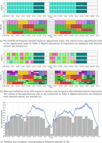
Figure 2(b) shows the best-case realisation of the base case blueprint schedule, which we obtained by optimally inserting the various trajectories in the base case blueprint schedule such that the expected waiting room occupancy is levelled. We determined this best-case realisation using the ILP with unlimited waiting room capacity, the levelling objective (as described in Section 3.3) and the subsequently described additional constraints. Observe from Table 3 that trajectories C – G and C-PA – G-PA have a similar colour tone, respectively, as their Stage 3 appointment type is identical. In the best-case realisation of the base case blueprint schedule these care trajectories are restricted to be scheduled into slots originally allocated to trajectories E and E-PA, respectively (hence the colours of E and E-PA already occurred in the blueprint schedule from Figure 2(a)).

4.1.2. Medical oncology & haematology clinic

During a typical day, the medical oncology & haematology clinic of UMCU is operated by four oncologists, one oncology PA, three haematologists and one haematology PA. The day-care department has 15 beds available for treatments (chemotherapy), operated by nurses. The morning shift starts at 8.30 h for physicians and at 9.00 h for PAs and ends at 12.00 h. Physicians and PAs both work their afternoon shift from 13.00 h until 17.00 h. Treatment is provided from 8.30 h until 17.00 h and appointments may be scheduled consecutively as staff members take lunch breaks in turn.

In the medical oncology & haematology clinic of UMCU a patient care trajectory consists of at least one and at most three stages. A patient has a scheduled consultation with a physician or PA (Stage 2), a treatment (Stage 3), or both. A consultation can be preceded by a blood test (Stage 1).

The clinic has two waiting areas. Patients bridging or waiting for an appointment with a physician or PA share a waiting room with 19 available seats. The waiting area at the day-care department, dedicated to patients waiting or bridging prior to treatment, has 16 available seats.

Based on a data-analysis of historical data, we identified 18 different patient care trajectories that occur, on average, at least once a day. Table 4 lists for every included trajectory the corresponding appointment type at each stage, whether it is possible to schedule these appointment(s) digitally, the corresponding minimum bridging times (if applicable), and the number of times this care trajectory is included in the case mix. Trajectories D – G belong to medical oncology, trajectories H – K belong to haematology and trajectories L – O represent single chemotherapy appointments (varying in duration) for which no specification of specialty is required. Both medical oncologists and haematologists distinguish two types of consultations (i.e. at Stage 2 there are two appointment types): new patients that take 40 min and follow-up consultations that take 20 min, all independent of whether a patient is seen by a physician or a PA. For duration of the chemotherapy treatments is included in Table 4. Note that only trajectories consisting of a single appointment at Stage 2 may be replaced with a digital appointment and that treatments always have to be performed in-person. The data analysis showed that patients that arrive from outside the clinic for an in-person appointment arrive 15 min early on average.

Table 4. Trajectories medical oncology & haematology clinic UMCU. For each trajectory the appointment type per stage is denoted together with the option to replace a consultation with a digital consultation, the minimum bridging times (in minutes) and the number of occurrences required in the blueprint schedule. The colour of a trajectory corresponds to the blueprint schedules in Figure 8(a) – 9(b).

Trajectory		Stage 1	Stage 2	Stage 3	Digital consultation possible?	Bridging time before Stage 2	Bridging time before Stage 3	Number of occurrences in blueprint
	A – oncology		New patient		Yes	–	–	10
	B – oncology		Follow-up		Yes	–	–	28
	C – oncology	Blood test	Follow-up		No	60	–	40
	D	Blood test	Follow-up	Chemo 60 min.	No	60	60	6
	E	Blood test	Follow-up	Chemo 90 min.	No	60	60	11
	F	Blood test	Follow-up	Chemo 120 min.	No	60	60	10
	G	Blood test	Follow-up	Chemo 210 min.	No	60	60	3
	A – haematology		New patient		Yes	–	–	8
	B – haematology		Follow-up		Yes	–	–	21
	C – haematology	Blood test	Follow-up		No	60	–	30
	H	Blood test	Follow-up	Chemo 30 min.	No	60	45	10
	I	Blood test	Follow-up	Chemo 60 min.	No	60	45	10
	J	Blood test	Follow-up	Chemo 120 min.	No	60	45	4
	K	Blood test	Follow-up	Chemo 180 min.	No	60	45	3
	L			Chemo 30 min.	No	–		3
	M			Chemo 60 min.	No	–	–	3
	N			Chemo 120 min.	No	–	–	3
	O			Chemo 210 min.	No	–	–	2

4.2. Case study results

4.2.1. Rheumatology clinic

To compare the outcomes of our results, we first analysed the expected waiting occupancy outcomes of the pre-COVID-19 best-case base case blueprint schedule of the rheumatology clinic of SMK. Figure 2(c) shows the predicted waiting room occupancy. In this figure, the peaks around 8.30 h and 13.00 h show the start of the new clinic sessions, and the peaks around 11.00 h and 16.00 h clearly shows the impac of bridging patients.

The blueprint schedule and waiting room occupancy for the SMK case study resulting from the ILP (1a) – (1i) with no additional objective functions is shown in Figure 3(a). For the given waiting room capacity of 18 seats, all patient trajectories are scheduled without replacing in-person appointments by digital appointments. The expected maximum waiting room occupancy is 17.

Figure 3. Optimal blueprint schedule (a) for the rheumatology clinic of SMK when only the number of in-person consultations is maximised; and the corresponding waiting room occupancy (b) for three variability settings. We refer to the caption of Figure 2 for a more detailed explanation of the figure.

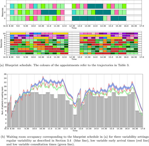
Figure 3(b) depicts the simulated waiting room occupancy of this blueprint schedule. To analyse the impact of reducing variability in patient punctuality and consultation duration, we simulated three variability settings: (1) regular variability, as described in Section 3.4; (2) low variable arrival times; and (3) low variable appointment durations. We observe that although the deterministic waiting room occupancy is below the maximum of 18 at all times, the simulated waiting room occupancy violates this considerably in case of regular variability, with peaks up to 24 patients. Furthermore we observe that reducing the variability in the arrival times does not significantly influence the maximum waiting room occupancy over time if the variability in appointment duration is not reduced as well. However, reducing the variability of the appointment durations reduces the maximum waiting room occupancy by approximately 10%.

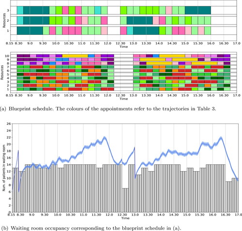
The deterministic waiting room occupancy for the blueprint schedule in Figure 3(a) varies considerably during the day. This suggests that the blueprint schedule can be adjusted to level the waiting room occupancy. Figure A depicts the blueprint schedule when the levelling objective (4) is considered. The ILP results show that all patient trajectories can be scheduled in-person. The expected maximum waiting room occupancy is reduced to 14. The simulated occupancy for this blueprint schedule is shown in Figure 4(a). Although the waiting room occupancy is reduced compared to the no-levelling blueprint schedule, the occupancy still exceeds the maximum of 18 for more than 2.5 h a day.

Figure 4. Optimal blueprint schedule (a) and waiting room occupancy (b) for the rheumatology clinic of SMK when the number of in-person consultations is maximised; the waiting room occupancy is levelled; and appointment types are evenly distributed over all resources. We refer to the caption of Figure 2 for a more detailed explanation of the figure.

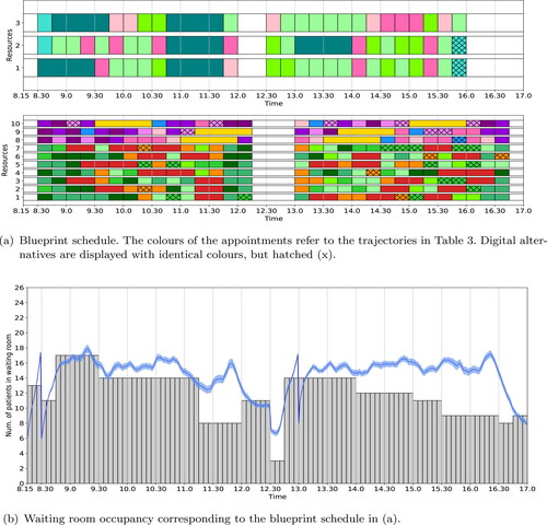
The next step in the iterative simulation optimisation approach is to reduce the waiting room capacity input parameters in the ILP, as mentioned in Section 3.1. If we reduce in a static way, iteratively solving the ILP shows that a minimal waiting area capacity of 11 seats is necessary to schedule all the patient care trajectories given the possibilities for digital consultations. Figure 5(a) shows the blueprint schedule and waiting room occupancy for this case with a waiting area capacity of 11. Here 25% of the previously scheduled in-person appointments are now replaced by digital appointments. The corresponding simulated waiting room occupancy is shown in Figure 5(b). Although the waiting room occupancy is further reduced, it is still exceeding the maximum capacity of 18 seats for approximately 60 min a day.

Figure 5. Optimal blueprint schedule (a) and waiting room occupancy (b) for the rheumatology clinic of SMK when the waiting room capacity is set to its minimum necessary to schedule all required occurrence for each trajectory. We refer to the caption of Figure 2 for a more detailed explanation of the figure.

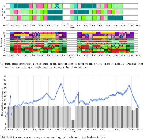
Comparing the simulated waiting room occupancy results for the various scenarios considered so far, shows an increase in waiting room occupancy deviation from the deterministically determined value as the clinic session progresses, both for the morning as well as afternoon sessions. Therefore, we expect that a time-dependent maximum waiting room capacity input that restricts the number of in-person appointments during these hours will reduce the actual waiting room occupancy. Therefore, we perform an experiment in which the available waiting room capacity is time-dependent, with the following settings: from 8.15 h-9.30h, 17 seats; 9.30 h-11.15h, 14 seats; 11.15 h-12.00h, 8 seats; 12.00 h-14.00h, 14 seats; 14.00 h-15.30h, 12 seats; 15.30 h-16.30h, 9 seats; and from 16.30h onwards, 17 seats. The resulting blueprint schedule is depicted in Figure 6(a), in which only 12% of the appointments are scheduled digitally. The simulated waiting room occupancy, as shown in Figure 6(b), never exceeds the maximum capacity of 18 seats.

Figure 6. Optimal blueprint schedule (a) and waiting room occupancy (b) for the rheumatology clinic of SMK with time-dependent restrictions on the number of patients simultaneously allowed in the waiting room. We refer to the caption of Figure 2 for a more detailed explanation of the figure.

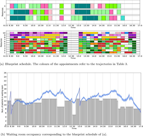
From Figure 6 it can be observed that it is a necessity to schedule in-person and digital appointments in an alternating fashion. If this is impossible to facilitate, an alternative approach for reducing the waiting room occupancy is to reduce the number of trajectories that are scheduled in the blueprint schedule. Figure 7(a) shows the blueprint schedule for the rheumatology department when the number of trajectories is reduced to 90% of the total case mix. This blueprint schedule is again created with time-dependent waiting room capacity restrictions, which determines where to leave an empty slot. Digital appointments are not necessary to meet the waiting room’s capacity restriction. The simulated waiting room occupancy is depicted in Figure 7(b). This result shows that reducing the case mix to 90% of its the total, reduces the waiting room occupancy in such a way that the maximum capacity is not exceeded. This is caused by reducing the number of care trajectories that have to be performed in-person, reducing the number of bridging patients.

Figure 7. Optimal blueprint schedule (a) and waiting room occupancy (b) for the rheumatology clinic of SMK when the number of trajectories is reduced to 90% of the total case mix. We refer to the caption of Figure 2 for a more detailed explanation of the figure.

In conclusion, the rheumatology clinic of SMK can continue to deliver 100% of their required daily appointments in times of COVID-19, given the restrictions to their shared waiting area. Their pre-COVID-19 best-case base case blueprint schedule results in peaks up to 25 patients in the waiting area, given that all patients are seen in-person. However, by introducing time-dependent waiting room capacity input restrictions our approach improves the waiting room occupancy such that the maximum capacity is no longer exceeded. As a consequence, 12% of the appointments is scheduled digitally and those digital appointments take place alternating with in-person appointments. If, for any reason, the rheumatology cannot this facilitate such sessions, or is not willing to perform this amount of appointments digitally, it is also possible to reduce the number of appointments in the case mix. If we reduce the number of appointments to 90% of the total case mix, Figure 7(a) shows a blueprint schedule, based on time-dependent waiting room capacity restrictions, that also ensures the maximum waiting room capacity is not exceeded and no digital appointments have to be scheduled.

4.2.2. Medical oncology & haematology clinic

The medical oncology & haematology clinic case study considers the situation with dedicated waiting areas for each stage. Solving the ILP (1a) – (1i) with no additional objectives, results in the blueprint schedules of Figures 8(a) and (b). For the given waiting room capacity of 19 seats at the outpatient clinic and 16 seats at the day-care department, a feasible schedule can be found in which none of the appointments are scheduled digitally. Figures 8(c) and (d) depict the simulated waiting room occupancy at the outpatient clinic and day-care department, respectively. From Figure 8(c) we conclude that the outpatient clinic waiting room is overcrowded for the majority of the day and only around the lunch break there is a period when the occupancy is acceptable. From Figure 8(d) we conclude that during the start of the day the waiting room occupancy at the day-care department is satisfactory and the difference between the deterministic waiting room occupancy and its simulated counterpart is small, while later during the day the occupancy is close to capacity (and even some short periods over capacity with at most one patient) and the difference between the deterministic waiting room occupancy and its simulated counterpart is increased. The increased difference between deterministic and simulated waiting room occupancy is because during the beginning of the day there are more idle periods and exclusively patients coming directly from home, hence treatment can start immediately upon arrival of the patient. Patients coming from the outpatient clinic are scheduled later during the day and must bridge a minimum amount of time between consultation and treatment. Hence, any delay at the outpatient clinic causes delay at the day-care department, which results in a increased difference between deterministic and simulated waiting room occupancy.

Figure 8. Optimal blueprint schedule of the outpatient clinic (a) and day-care department (b) for the medical oncology & haematology clinic in UMCU when only the number of in-person consultations is maximised. Along the x-axis is the time and along the y-axis is the resource (in (a) resources 1 – 4 and 5 represent the oncologists and oncology PA, resp., and resources 6 – 8 and 9 represent the haematologists and haematology PA, resp.). In (c) and (d) the waiting room occupancy for the outpatient clinic and day-care department, resp., is depicted over time. Here the grey bars denote waiting room occupancy levels taking into account bridging and average early arrival times (result from the ILP) and the blue line, together with its 95% confidence interval as the shaded area, depicts the waiting room occupancy including randomness in early arrival and consultation times (result form the MCS).

In the second iteration of our iterative simulation optimisation approach, we restrict the waiting area capacity input parameters during the hours the simulated waiting room occupancy peaks and used the levelling objective (4). The characteristics of the clinic cause that the waiting room capacity cannot easily be defined per 15 min or half an hour, but that it must be done for irregular time-intervals, sometimes even for just a single time-slot of 5 min. We omit the list of waiting room capacity over time, as the set capacity is attained by the resulting deterministic waiting room occupancy and, hence, can be observed from Figure 9(c). We will discuss below how we defined the waiting room capacity at the day-care department.

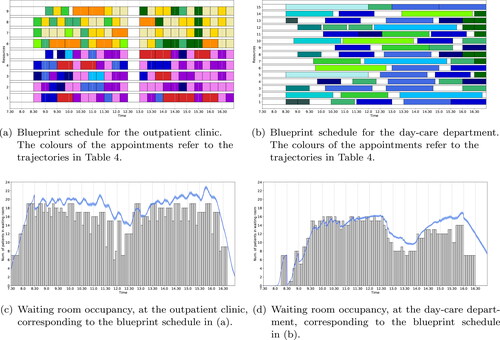
Figure 9. Optimal blueprint schedule of the outpatient clinic (a) and day-care department (b) for the medical oncology & haematology clinic in UMCU with time-dependent restrictions on the number of patients simultaneously allowed in the waiting rooms. The corresponding waiting room occupancy is shown in (c) and (d), resp. We refer to the caption of Figure 8 for a more detailed explanation of the figure.

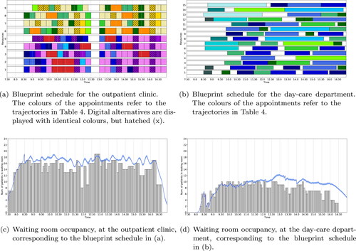
The resulting blueprint schedules are shown in Figures 9(a) and (b), where 22% of the appointments at the outpatient clinic are scheduled digitally (of all appointments a maximum of 35% could be scheduled digitally). In particular, 89% of C – oncology appointments and 81% of C – haematology appointments are scheduled digitally. The corresponding simulated waiting room occupancy at the outpatient clinic, respectively the day-care department is depicted in Figure 9(c) and (d). From Figure 9(c), it can be observed that, although during the peak moments the occupancy is really close to capacity, the waiting room occupancy at the outpatient clinic never violates its capacity of 19 seats. Furthermore, in Figure 8(d), we observe the waiting room occupancy at the day-care department to be around eight patients at 17.00 h, which may cause the day-care department to finish the session in overtime. Hence, in the second iteration of our iterative simulation optimisation approach we set the waiting room capacity at the day-care department time-dependently to its minimum required to get a feasible blueprint schedule that also satisfies the capacity restriction at the outpatient clinic. This resulted in the following settings: from 7.30h-14.30h, 10 seats; 14.30h-16.00h, 7 seats; 16.00h-16.15h, 4 seats; and from 16.15h onwards, 3 seats. With this settings, we observe from Figure 9(d) the waiting room at the day-care capacity never violates its capacity and the occupancy at 17.00 h is reduced to approximately five patients. This suggest the session still resorts to overtime to finish and it would be preferred to even further reduce the waiting room capacity at particularly the end of the day. By experimenting we observed that this preferred capacity reduction results in either infeasibility of the ILP (because treatments need to be scheduled near the end of the day in order to meet the waiting room capacity restriction at the outpatient clinic); or in overcrowding the waiting room occupancy at the outpatient clinic during periods of the day.

In conclusion, the medical oncology & haematology clinic of UMCU can continue to deliver 100% of their required daily appointments in times of COVID-19, given the restrictions to their dedicate waiting rooms. As a consequence, 22% of the appointments at the outpatient clinic is scheduled digitally and those digital appointments take place alternating with in-person appointments. At the day-care department, the afternoon session might need to be extended.

5. Conclusion

In this paper, we have proposed an iterative simulation optimisation approach, combining Integer Linear Programming (ILP) and Monte Carlo simulation (MCS), to develop a blueprint schedule for appointment systems, taking into account capacity restrictions in waiting areas and care trajectories. Although blueprint optimisation is widely considered in literature, including the waiting room occupancy as the main restriction is not yet considered. Due to distancing measures induced by the COVID-19 pandemic, including this metric in blueprint optimisation, as proposed in this paper, became very relevant. Besides positioning appointments in the blueprint schedule, our model also determines which appointments need to be scheduled digitally to meet the waiting area capacity restrictions under COVID-19 distancing measures.

The main assumption that makes our ILP model tractable is that early arrival times and appointment durations are deterministic. Although this assumption is common for development of blueprint schedules, it is not realistic in practice. Therefore, our MCS model investigates the quality of the ILP schedule under randomness in early arrival times and appointment durations. Furthermore, our iterative approach allows for inclusion of the effects of these random durations and early arrival times in the ILP blueprint schedule by adapting the available waiting area capacity in certain time slots, enforcing the ILP to schedule appointments in slots that reduce the occupancy of the waiting area. The new schedule is investigated using our MCS model, and if required further adapted.

Our approach is very generic and can be applied to outpatient clinics with various characteristics, as we show by our case studies. For our case study clinics, all patient appointments of the case mixes can be scheduled, while meeting the capacity restrictions, by scheduling at most 12% and 22% of the appointments digitally. We also showed that for our case study clinics, a focus on reducing the variability of appointment durations is preferred over reducing patient arrival variability, when considering waiting room occupancy as our main restriction.

Our ILP model can be easily extended to determine the optimal number of appointments, given a desired number of appointments per type. Our MCS model can also be used on an operational level of control for waiting room occupancy steering. Instead of evaluating a blueprint with patient types, actual scheduled patients and the characteristics of their pathways can be evaluated with the same model, to determine the expected occupancy on a short term (today/tomorrow). Our results may also reveal the impact on waiting area occupancy of interventions such as improving schedule execution, and patient and provider punctuality. Other interventions might further reduce the bridging time. For example, in advance drug preparation might decrease the patient bridging times, at the cost of occasionally wasting medications (Masselink et al., 2012). Introducing next-day appointment schedules, for example when patients have their diagnostic tests one day before the outpatient clinic appointments (Dobish, 2003), decouples the same-day appointments and may also reduce waiting area occupancy as it avoids bridging times. The impact of such interventions on waiting area occupancy may be characterised using our method.

Patients requiring non-COVID-19 care in times of COVID-19 are typically requested to visit the hospital unaccompanied. However, for specific patient types, such as children and elderly, patients with physical discomfort or consultations to discuss unfavourable outcomes, an accompanying person will join the patient during the hospital visit. This puts additional pressure on the waiting area, even in the case this accompanying person is allowed within 1.5 meters of the patient. In setting the waiting area capacity limits for the blueprint design, the impact of accompanying people has to be taken into account. If a patient wants to bring an accompanying person, the MCS results of the blueprint schedule may give more insight in which slot to select such that the waiting area occupancy does not exceed its limits.

Besides well performing blueprint schedules that incorporate waiting area restrictions, our approach also provides hospitals with more insight in the decisions they make regarding their case-mix and care trajectory design. Besides medically relevant same-day trajectories, most same-day multi-appointment trajectories that hospitals pre-COVID-19 used to offer are considered a service to their patients, for example to limit the amount of hospital visits. Our research shows that the choice for coupled (same-day) instead of decoupled (multi-day) patient trajectories, or same-day trajectories with large minimum bridging times compared to no minimum bridging times, may come at a cost of reduced patient volume in times of COVID-19. Our methods therefore aided decision makers of our case study hospitals in finding the mix of same-day and multi-day trajectories that allowed them to safely serve their patients in times of COVID-19.

Additional information

Funding

This project is partly financed by the Netherlands Organisation for Health Research and Development (ZonMw) under grant number 10430042010015.

Appendix A.

Monte Carlo simulation

Simulation optimisation refers to solving an ILP model with stochastic elements (Karatas et al., 2017; Santos et al., 2017). In many cases simulation is used to estimate the objective function (Fu, 2015). In our model, variability is introduced via the early arrival times and the duration of consultation. This variability does not affect the value of the objective function, but may cause the waiting area capacity constraints to be violated. Our MCS determines bounds for these constraints such that the probability that they are violated is less than 5%. Our approach therefore falls in the subcategory of Stochastic Constraints Simulation (Homem-de Mello & Bayraksan, 2015).

The outline of the MCS is as follows. At initialisation, the blueprint schedule obtained from the ILP is loaded in the simulation and the early arrival, consultation and treatment times are generated for every patient of that arrive during the day. These randomly generated numbers are then used to obtain the effectuated schedule by determining the actual arrival times of the patients and the starting times of the consultations and treatments. Subsequently, the simulation determines for every time step if a patient is present in the system and if so whether or not that patient is currently in consultation or treatment. This determines, for each time step, the number of patients in the waiting area. After a predetermined number of repetitions a 95% confidence interval is obtained. The pseudo code of the MCS is as follows:

Table

Algorithm 1: Monte Carlo simulation to evaluate waiting area occupancy of blueprint schedule

References

- Ahmadi-Javid, A., Jalali, Z., & Klassen, K. J. (2017). Outpatient appointment systems in healthcare: A review of optimization studies. European Journal of Operational Research, 258(1), 3–34. https://doi.org/10.1016/j.ejor.2016.06.064
- COVIDSurg Collaborative. (2020). Elective surgery cancellations due to the COVID-19 pandemic: Global predictive modelling to inform surgical recovery plans. British Journal of Surgery, 107(11), 1440–1449.
- Cox, J. F., III, & Boyd, L. H. (2018). Using the theory of constraints' processes of ongoing improvement to address the provider appointment scheduling system design problem. Health Systems (Basingstoke, England), 9(2), 124–158. https://doi.org/10.1080/20476965.2018.1471439
- Currie, C. S., Fowler, J. W., Kotiadis, K., Monks, T., Onggo, B. S., Robertson, D. A., & Tako, A. A. (2020). How simulation modelling can help reduce the impact of COVID-19. Journal of Simulation, 14(2), 83–15. pageshttps://doi.org/10.1080/17477778.2020.1751570
- da Silva, F. C. T., & Barbosa, C. P. (2021). The impact of the COVID-19 pandemic in an intensive care unit (ICU): Psychiatric symptoms in healthcare professionals. Progress in Neuro-Psychopharmacology and Biological Psychiatry, 110, 110299. https://doi.org/10.1016/j.pnpbp.2021.110299
- Dobish, R. (2003). Next-day chemotherapy scheduling: A multidisciplinary approach to solving workload issues in a tertiary oncology center. Journal of Oncology Pharmacy Practice, 9(1), 37–42. https://doi.org/10.1191/1078155203jp105oa
- Emanuel, E. J., Persad, G., Upshur, R., Thome, B., Parker, M., Glickman, A., Zhang, C., Boyle, C., Smith, M., & Phillips, J. P. (2020). Fair allocation of scarce medical resources in the time of covid-19. The New England Journal of Medicine, 382(21), 2049–2055. https://doi.org/10.1056/NEJMsb2005114
- Fu, M. C. (2015). Handbook of simulation optimization. Springer International Publishing.
- González-Gil, M. T., González-Blázquez, C., Parro-Moreno, A. I., Pedraz-Marcos, A., Palmar-Santos, A., Otero-García, L., Navarta-Sánchez, M. V., Alcolea-Cosín, M. T., Argüello-López, M. T., Canalejas-Pérez, C., Carrillo-Camacho, M. E., Casillas-Santana, M. L., Díaz-Martínez, M. L., García-González, A., García-Perea, E., Martínez-Marcos, M., Martínez-Martín, M. L., del Pilar Palazuelos-Puerta, M., Sellán-Soto, C., & Oter-Quintana, C. (2021). Nurses’ perceptions and demands regarding COVID-19 care delivery in critical care units and hospital emergency services. Intensive & Critical Care Nursing, 62, 102966.
- Homem-de Mello, T., & Bayraksan, G. (2015). Stochastic constraints and variance reduction techniques. In M. C. Fu (Ed.), Handbook of simulation optimization (chapter 9, pp. 245–276). Springer International Publishing.
- Hulshof, P. J. H., Kortbeek, N., Boucherie, R. J., Hans, E. W., & Bakker, P. J. M. (2012). Taxonomic classification of planning decisions in health care: A structured review of the state of the art in or/ms. Health Systems, 1(2), 129–175. https://doi.org/10.1057/hs.2012.18
- Karatas, M., Razi, N., & Gunal, M. M. (2017). An ILP and simulation model to optimize search and rescue helicopter operations. Journal of the Operational Research Society, 68(11), 1335–1351. https://doi.org/10.1057/s41274-016-0154-7
- Kortbeek, N., van der Velde, M., & Litvak, N. (2017). Organizing multidisciplinary care for children with neuromuscular diseases at the academic medical center, Amsterdam. Health Systems, 6(3), 209–225. https://doi.org/10.1057/s41306-016-0020-5
- Lamé, G., Jouini, O., & Stal-Le Cardinal, J. (2016). Outpatient chemotherapy planning: A literature review with insights from a case study. IIE Transactions on Healthcare Systems Engineering, 6(3), 127–139. https://doi.org/10.1080/19488300.2016.1189469
- Leeftink, A., Bikker, I., Vliegen, I., & Boucherie, R. (2018). Multi-disciplinary planning in health care: A review. Health Systems (Basingstoke, England), 9(2), 95–118. https://doi.org/10.1080/20476965.2018.1436909
- Liang, B., Turkcan, A., Ceyhan, M. E., & Stuart, K. (2015). Improvement of chemotherapy patient flow and scheduling in an outpatient oncology clinic. International Journal of Production Research, 53(24), 7177–7190. https://doi.org/10.1080/00207543.2014.988891
- Lin, C. K. Y., Ling, T. W. C., & Yeung, W. K. (2017). Resource allocation and outpatient appointment scheduling using simulation optimization. Journal of Healthcare Engineering, 2017, 9034737. https://doi.org/10.1155/2017/9034737
- Marynissen, J., & Demeulemeester, E. (2019). Literature review on multi-appointment scheduling problems in hospitals. European Journal of Operational Research, 272(2), 407–419. https://doi.org/10.1016/j.ejor.2018.03.001
- Masselink, I. H., van der Mijden, T. L., Litvak, N., & Vanberkel, P. T. (2012). Preparation of chemotherapy drugs: Planning policy for reduced waiting times. Omega, 40(2), 181–187. https://doi.org/10.1016/j.omega.2011.05.003
- Mes, M. R. K., Vliegen, I. M. H., & Doggen, C. J. M. (2021). A quantative analysis of integrated emergency posts. In M. E. Zonderland, R. J. Boucherie, E. Hans, & N. Kortbeek (Eds.), Handbook of healthcare logistics, bridging the gap between theory and practice (chapter 11, pp. 201–230). Springer International Publishing.
- RIVM. (2020). Major increase in hospital admissions and ICU admissions due to covid-19. Retrieved April 14, 2021, from https://www.rivm.nl/en/news/Major-increase-in-hospital-admissions-and-ICU-admissions-due-to-COVID-19.
- Santos, N., Tubertini, P., Viana, A., & Pedroso, J. P. (2017). Kidney exchange simulation and optimization. Journal of the Operational Research Society, 68(12), 1521–1532. https://doi.org/10.1057/s41274-016-0174-3
- van Giessen, A., de Wit, A., van den Brink, C., Degeling, K., Deuning, C., Eeuwijk, J., van den Ende, C., van Gestel, I., Gijsen, R., van Gils, P., IJzerman, M., de Kok, I., Kommer, G., Kregting, L., Over, E., Rotteveel, A., Schreuder, K., Stadhouders, N., & Suijkerbuijk, A. (2020). Impact van de eerste COVID-19 golf op de reguliere zorg en gezondheid: Inventarisatie van de omvang van het probleem en eerste schatting van gezondheidseffecten. Rijksinstituut voor Volksgezondheid en Milieu (RIVM). [Report in Dutch; English abstract provided].
- Wehrle, C. J., Lee, S. W., Devarakonda, A. K., & Arora, T. K. (2021). Patient and physician attitudes toward telemedicine in cancer clinics following the COVID-19 Pandemic. JCO Clinical Cancer Informatics, 5(5), 394–400. PMID: 33822651.
- Wu, K., Darcet, D., Wang, Q., & Sornette, D. (2020). Generalized logistic growth modeling of the COVID-19 outbreak: Comparing the dynamics in the 29 provinces in China and in the rest of the world. Nonlinear dynamics, 101(3), 1561–1581.
- Yang, K.-K., & Cayirli, T. (2020). Managing clinic variability with same-day scheduling, intervention for no-shows, and seasonal capacity adjustments. Journal of the Operational Research Society, 71(1), 133–152. https://doi.org/10.1080/01605682.2018.1557023
- Zonderland, M. E. (2021). Theoretical and practical aspects of outpatient clinic optimization. In M. E. Zonderland, R. J. Boucherie, E. Hans, & N. Kortbeek (Eds.), Handbook of healthcare logistics, bridging the gap between theory and practice (chapter 3, pp 25–36). Springer International Publishing.
- Zonderland, M. E., & Boucherie, R. J. (2021). A survey of literature reviews on patient planning and scheduling in healthcare. In M. E. Zonderland, R. J. Boucherie, E. Hans, & N. Kortbeek (Eds.), Handbook of healthcare logistics, bridging the gap between theory and practice (chapter 2, pp. 17–24). Springer International Publishing.
- Zonderland, M. E., Boucherie, R. J., Hans, E., & Kortbeek, N. (2021). Handbook of healthcare logistics. Bridging the gap between theory and practice. Springer International Publishing.