Choosing where to set the threshold between low- and high-risk patients: Evaluating a classification tool within a simulation

Abstract

Health service providers must balance the needs of high-risk patients who require urgent medical attention against those of lower-risk patients who require reassurance or less urgent medical care. Based on their characteristics, we developed a tool to classify patients as low- or high-risk, with correspondingly different patient pathways through a service. Rather than choosing the threshold between low- and high-risk patients solely considering classification accuracy, we demonstrate the use of discrete-event simulation to find the best threshold from an operational perspective as well. Moreover, the predictors in classification tools are often categorical, and may be inter-dependent. Defining joint distributions of these variables from empirical data assumes that missing combinations are impossible. Our new approach involves using Poisson regression to estimate the joint distributions in the underlying population. We demonstrate our methods on a practical example: setting the threshold between low- and high-risk patients with proposed different pathways through a breast diagnostic clinic.

Keywords:

• Simulation
• health services
• risk
• credit scoring
• regression

1. Introduction

Healthcare budgets constantly have to address the increased demand for the array of diagnostic tests and treatments for patients with cancer because the successes of research and development in care and diagnostics have led to more people living longer. Health service providers must balance the needs of high-risk patients who require urgent medical attention against those of lower-risk patients who require reassurance or less urgent medical care. Classification methods, for example logistic regression or decision trees, can be used to predict whether a patient is at low or high risk of a disease. Then these patients can be routed along low- or high-risk pathways through health services, recognising the different needs of these two patient groups.

When using these classification methods, managers must choose where to set the threshold between low- and high-risk patients. Solely basing this decision on classification accuracy (for example sensitivity or specificity measures), neglects the operational impact of implementing risk-based pathways (for example waiting times or resource use). In this paper, we propose using discrete-event simulation, in addition to estimating classification accuracy, to help choose the threshold that provides the best results from an operational perspective.

When evaluating risk-based patient management strategies in discrete-event simulation models, the way in which patient characteristics are modelled requires careful consideration. Patient characteristics affect not only the patient’s risk group, but also the patient’s route through the simulation, as well as potentially their priority in queues and service times. Patient characteristics are often categorical and inter-dependent. Some possible combinations of characteristics may not appear in a data sample, but may exist in the wider population. We propose an approach using Poisson loglinear (regression) models for generating combinations of dependent categorical characteristics, allowing generation of missing combinations.

We demonstrate our approach with a case study of a breast diagnostic clinic. The classification tools developed, in this case logistic regression scorecards, are built from data extracted from forms completed by general practitioners (GPs) referring patients to the clinic. Currently all patients follow the same pathway through the clinic; we investigate a proposal for patients classified as being at high risk of an abnormal result, and thus needing diagnostic tests, to take a different pathway from low-risk patients. Our method evaluates the classification tools in a simulation which routes patients along low- and high-risk pathways through the clinic. Our aim is to find appropriate threshold risk scores (cut-off scores) above which patients should be considered high-risk. As this is a preliminary study, with data from a limited number (n = 179) of patients, not all the possible combinations of patient characteristics are present in the data. We therefore use our method of Poisson regression to generate combinations of characteristics within the simulation. We compare results in terms of clinic efficiency (proportion of time spent in consultations or tests) and patients’ total time at the clinic.

Although many researchers have applied operational research techniques to cancer care, operational research studies addressing cancer diagnostic services are rare (Saville et al., 2019), aside from tools for predicting cancer risk. Also, limited research spans both primary and secondary cancer care services (Saville et al., 2019).

The main contributions of this paper from a theoretical and practical perspective are

• Combining classification and discrete-event simulation to find the best result considering both predictive accuracy and operational performance

• Poisson regression for modelling combinations of characteristics that do not necessarily appear in the sample

• Showing how GP referral information can be used to triage patients while still giving all patients the chance to have tests if a clinician decides they are needed

The paper proceeds as follows. In Section 2, we present a brief overview of relevant literature. In Section 3 we describe the healthcare background and the case study setting. Section 4 details the approach used, including the development of the logistic regression scorecards, a description of the simulation model and our method for generating patient labels for simulation. In Section 5, we present the classification accuracy and operational performance of different cut-off scores. In Section 6, we discuss the contributions and limitations of the study, with future research directions. The conclusion is given in Section 7.

2. Literature review

Over the last two decades, several authors have combined patient classification techniques with discrete-event simulation (Bhattacharjee & Ray, 2016; Cannon et al., 2013; Harper, 2002; Harper et al., 2003; Huang & Hanauer, 2016). Some of these researchers used classification to model patient pathways accurately, by generating groups of similar patients as simulation inputs (Harper, 2002) or predicting the occurrence of health-related events during the simulation (Cannon et al., 2013; Harper et al., 2003). On the other hand, Bhattacharjee and Ray (2016) classified patients using a Classification and Regression Tree and then used discrete-event simulation to evaluate the potential impact of sequencing appointments based on the patient classes. Huang and Hanauer (2016) present a series of logistic regression models to predict no-shows. Each model contains information about one more prior attendance, and can be used to decide to what extent to overbook appointments. Here, discrete-event simulation was used to evaluate the cost (waiting time plus overtime plus idle time) per patient for these different models, and so to decide how many prior attendance variables should be included. Unlike these papers, we describe how discrete-event simulation can help choose the threshold score above which patients should be classified as high-risk.

Another relevant body of literature relates to setting thresholds in classification algorithms when there are asymmetric costs (Pazzani et al., 1994, Zhao, 2008). This is the case when misclassifying is worse in one direction than the other, so sensitivity may be more important than specificity or vice versa. Many papers have built classification models for predicting breast cancer, for example Ayer et al. (2010), Mangasarian et al. (1995), and Pendharkar et al. (1999). Unlike these, we are using classification models for predicting any kind of abnormal result, including but not limited to cancer, from imperfect information (GP referrals). This is to help with identifying which patients are likely to need imaging tests. In our context, the cost of a missed abnormal result is also not as extreme as missing a cancer case – these misclassified patients are sent to see a clinician who is still able to send the patient for imaging tests (as today).

In simulation models of pathways through healthcare services, researchers have modelled patient characteristics in three main ways (sometimes in combination). One way is grouping patients with similar characteristics, either by specifying the probability of belonging to each group (Bayer et al., 2010; Chemweno et al., 2014; Crawford et al., 2014), or by using group-specific arrival rates (Cooper et al., 2002; Gillespie et al., 2016; Monks et al., 2016). The relative numbers of patients in each group are sometimes based on expert opinion (Chemweno et al., 2014) or assumed to be the same as in data samples (Cooper et al., 2002; Crawford et al., 2014). When the choice of groups is not obvious, patient data can be analysed to find appropriate groups, for example Gillespie et al. (2016) group patients with similar lengths of stay using Kaplan-Meier and log-rank tests. Elsewhere, different clustering (Ceglowski et al., 2007; Isken & Rajagopalan, 2002) and classification (Harper, 2002) techniques have been used to group similar patients. These approaches provide insufficiently detailed characteristics for our situation.

A second way of modelling patient characteristics is inputting empirical data, either by putting each real patient’s information directly into the discrete-event simulation (Eatock et al., 2011; Khanna et al., 2016), bootstrapping (Lord et al., 2013) or generating copies of each patient's set of characteristics to compare different treatment strategies on the same cohort (Revankar et al., 2014). The drawback of directly using empirical data is that it only includes those patients seen in reality. This approach is therefore most suitable when the data sample is deemed large enough to closely resemble the underlying population.

A third approach to this problem is using statistical distributions, either assuming independence between characteristics (Burr et al., 2012; Crane et al., 2013; Tran-Duy et al., 2014), or relationships between some characteristics (Cooper et al., 2002; Lord et al., 2013; Pilgrim et al., 2009; Vataire et al., 2014; Wang et al., 2017). These papers either use the empirical conditional distributions present in their data or make assumptions about the relationships when data are unavailable. Using the empirical conditional distribution relies on the relationships present in the sample being representative of the wider population; combinations of characteristics not present in the sample will not be simulated. In contrast, we propose an approach for generating combinations of dependent, categorical characteristics, where combinations not present in the data sample may be simulated.

3. Healthcare background and case study

Breast cancer is the most common cancer in the UK, making up 15% of new cancer cases, with 99% of cases affecting women (Cancer Research UK, 2016b). Survival is improving, with 85% of women diagnosed in England and Wales surviving the disease for at least five years. However, the stage at which a cancer is detected greatly impacts chances of survival, with only 26% of women with final stage disease surviving beyond 5 years (Cancer Research UK, 2018).

The most common route to breast cancer diagnosis is via referral by a General Practitioner (GP) to a specialist diagnostic clinic, accounting for 60% of diagnoses (Cancer Research UK, 2016a). These clinics are under strain; the covid-19 pandemic has caused a backlog for cancer diagnostic services (Hanna et al., 2020).

Currently, diagnostic clinics are organised as follows. A two-week wait target between when a patient is referred and their attendance in clinic (Keogh, 2009) recognises the urgency of confirming or eliminating a cancer diagnosis for both physical and mental reasons. One-stop clinics are recommended, i.e., they should offer all necessary diagnostic tests on a single day (Willett et al., 2010). Two main options exist for organising the sequence of services within the day. In some clinics, staff use information provided by GPs on referral to identify those patients who should be sent straight for imaging tests. The remaining patients are sent to see a clinician who decides whether to request imaging. In other clinics, all patients see a clinician first. In this case, the information provided by GPs may not be used at all.

All patients visiting breast diagnostic clinics will be worrying about the possibility of cancer, although only a small proportion will receive a breast cancer diagnosis, for example 4% of patients included in this study. Cancer is the most feared serious illness, with women fearing breast cancer second most after brain cancer, according to a survey commissioned by Cancer Research UK (2011). Clinic visits involve multiple stages, meaning patients may wait multiple times, with little distraction from contemplating their potential diagnosis. Thus, it is important that the proportion of time patients spend in consultations and tests (where appropriate), as opposed to waiting between stages and queuing, should be as high as possible. Moreover, it is critical that patients receive a diagnosis confirming or excluding cancer as quickly as possible on the day of their clinic visit.

The case study is based at the Whittington Health NHS Trust in North London, which provides hospital and community services to a population of 500,000 in Islington, Haringey, Barnet, and Camden (Whittington Health NHS, 2019a). The Whittington Hospital runs a one-stop clinic for diagnosis of patients with breast symptoms (Whittington Health NHS, 2019b). In this clinic, all patients see a clinician first. We model the potential operational impact of implementing risk-based pathways at this clinic.

4. Materials and methods

Our methods and data sources are outlined here; further details are available in the supplemental material.

4.1. Data sources

Between November 2015 and December 2016, patients were asked to fill in questionnaires about the time they spent in different stages of their appointment (n = 99). This was complemented with a time and motion study where service and turnaround times were measured by the PhD student.

Separately, between January and March 2016, we asked for patients’ consent to use their anonymised records to create a unique dataset linking GP referral information to clinic tests and results. This dataset (n = 179) was used both for developing the scorecards and for generating patient labels to determine each patient’s route through the simulation.

4.2. Logistic regression scorecards to predict patient risk

As classification tools, we develop two alternative logistic regression models that use GP referral information to separate patients into groups at low and high risk of having an abnormal result. For ease of interpretability, we transform the logistic regression models into scorecards, using the “weights of evidence” approach common in credit scoring applications (Thomas, 2009). Scorecards can be represented on an arbitrary linear scale, are particularly suitable when the concept of risk is involved and make the same predictions as the original logistic regression models. In this last respect scorecards differ from the points system method proposed by Sullivan et al. (2004), used for example as a breast cancer prediction rule (McCowan et al., 2011), where the points system provides an approximation to the original model.

We considered the following seven commonly-reported characteristics for inclusion as predictors in our model: “family history of cancer,” “lump,” “unilateral pain” (one-sided pain), “other symptom,” “urgency,” “duration of symptoms,” and “age.” The characteristic “other symptom” refers to rarer symptoms (those present in 15 or fewer cases).

The outcome, a “normal” (Y = 1) or “abnormal” (Y = 0) diagnostic result, was derived from patients’ test results. A normal result means the patient has healthy breasts or does not require imaging. Abnormal results cover both cancer and benign breast diseases, including benign breast lumps such as cysts and fibroadenomas, infections (for example mastitis and abscesses), and congenital problems, which cause the breast to have an abnormal external appearance (Harvey et al., 2014). Distinguishing between cancer and non-cancerous diseases without imaging is difficult (Harvey et al., 2014), which is why we propose routing patients at high risk of having an abnormal result to imaging first.

A binary logistic regression model predicts the probability, p, of a normal result from patient-specific variables, X₁, X₂, … X_n, obtained from GP referral information, as given in Equation 1(1) $$\begin{array}{c}p≔\mathit{Prob}\left(Y=1\right|X_1,X_2,\dots ,X_n)=\frac{1}{1+e^{-\left({\beta }_0+{\sum }_{i=1}^n{\beta }_i{X}_i\right)}}\end{array}$$(1) . The parameters β₁, β₂, … β_n show the relative importance of each characteristic in the prediction and β₀ is the intercept. These parameters are obtained from maximum likelihood estimates. In reality, there is some error, ε, that is not captured by the model. (1) $$\begin{array}{c}p≔\mathit{Prob}\left(Y=1\right|X_1,X_2,\dots ,X_n)=\frac{1}{1+e^{-\left({\beta }_0+{\sum }_{i=1}^n{\beta }_i{X}_i\right)}}\end{array}$$(1)

The weight of evidence, W, of a particular grouped attribute j, for example “young,” of a characteristic i, for example “age,” is the strength of evidence that patients who have the attribute will have an abnormal result. Let the number of normal (abnormal) results with attribute j be n_j (a_j) and the total number of normal (abnormal) results be n_total (a_total). Then the weight of evidence variable, W_ij, is given by the following. (2) $$\begin{array}{c}{W}_{ij}=\ln \left(\frac{a_j}{a_{\mathit{total}}}÷\frac{n_j}{n_{\mathit{total}}}\right)\end{array}$$(2)

The scaled score, S, which is calculated from a scorecard, is related to the unscaled score, ${\beta }_0+{\sum }_{i=1}^n{\beta }_i{X}_i,$ which appears in the logistic regression, as follows. (3) $$\begin{array}{c}S=\left({\beta }_0+{\sum }_{i=1}^n{\beta }_i{X}_i\right)\cdot \text{factor}+\text{offset}\end{array}$$(3)

The factor and offset are the solution to the following system of linear equations. This follows since the unscaled score is equal to the log odds. The pair (Score, Odds) is the alignment point, e.g., it is assumed that the score 300 corresponds to odds of 12(:1) of having an abnormal result. The PDO is the specified number of points to double the odds, e.g., if PDO is 20, then the odds double for every increase in 20 points. (4) $$\begin{array}{c}\text{Score}=\ln \left(\text{Odds}\right)\cdot \text{factor}+\text{offset}\end{array}$$(4) (5) $$\begin{array}{c}\text{Score}+\text{PDO}=\ln \left(2\cdot \text{Odds}\right)\cdot \text{factor}+\text{offset}\end{array}$$(5)

Using the weights of evidence codings as the X variables, the scaled score for a particular patient becomes (6) $$\begin{array}{c}S=\left({\beta }_0+\sum _{i=1}^n{\beta }_i{W}_{ij}\right)\cdot \text{factor}+\text{offset}\end{array}$$(6) where n is the number of variables and j is the attribute that this patient has for characteristic i.

The points of the scaled score can be split between the characteristics by dividing the parts of the score that are not characteristic-specific between them. (7) $$\begin{array}{c}\text{Points for characteristic }i=\left(\frac{{\beta }_0}{n}+{\beta }_i{W}_{ij}\right)\cdot \text{factor}+\frac{\text{offset}}{n}\end{array}$$(7) Finally, to find the total score for a particular patient, the points for each of the patient's attributes are added up.

Models were developed in SAS Enterprise Miner 14.1 software. We developed two models: a full scorecard containing seven characteristics and a simple scorecard containing fewer characteristics. We selected variables for inclusion in the simple scorecard based on their information values, which measure how much each variable contributes to the abnormality prediction (Thomas, 2009). The simple scorecard contains only the two most predictive characteristics, “lump” and “age” which are strong and medium predictors of abnormal results, respectively (SAS, 2013). Values of the two continuous characteristics, “duration of symptoms” and “age” were grouped into attributes using the Interactive Grouping feature. This feature automatically generates groups using a decision tree algorithm aiming to maximise patient similarity (in terms of diagnostic results) within groups. For example, perfect similarity (technically, zero entropy) would mean that all patients in a group had the same diagnostic result. Such grouping helps build more parsimonious and robust models that can capture non-monotonic relationships. For the simple scorecard, the age groups were adapted to 10-year brackets for ease of use.

Since the sample size is relatively small (n = 179 patients), the scorecards were estimated using the entire dataset to make use of all the available data, rather than removing some to use in validation. Instead, a bootstrapping technique (sampling with replacement), implemented in Microsoft Excel, was used to internally validate the models.

4.3. Simulation modelling

The simulation models patients' visits to the clinic, from arrival to discharge (see Figure 1). Waits are omitted from the figure but are potentially present between each stage. Patients who are predicted abnormal results (have scores at least as high as the cut-off score) are sent straight for imaging tests; otherwise patients see a clinician first. In the simulation, we ignored the small numbers of patients who are ineligible for the scorecard (males and non-GP referrals), and assumed referral information would be provided for all patients.

Figure 1. Simulation process map. DNA = Did not attend.

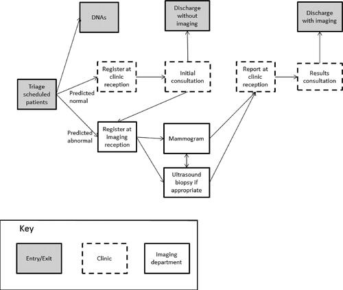
Patients have the following imaging tests. It is assumed that imaging first patients (those that are predicted an abnormal result) are given the same imaging tests as those patients with actual abnormal results in our data, dependent on age (see Table 3 in the Supplemental material). For the clinician first patients (those patients predicted normal results), we assume clinician behaviour in requesting tests remains unchanged from current behaviour. That is, we assume the same test proportions as in the data, dependent on age and actual result (see Tables 3 and 4 in the Supplemental material). It is assumed that patients with actual normal results never have a biopsy. Of those patients with actual abnormal results who have an ultrasound, we assume 44% also have a biopsy, as in our dataset.

Patients are prioritised for tests in the simulation in the following way. For mammograms, patients who have had an ultrasound are prioritised in order of waiting time. Then other patients are seen in order of their waiting time, regardless of whether they have come from a consultation or straight for imaging. Similarly, for ultrasound, patients who have had a mammogram are prioritised in order of waiting time. Then other patients are seen in order of their waiting time, again regardless of whether they visited a clinician or imaging first. In terms of prioritising patients to see a clinician, we observed different prioritisation behaviours, so experimented with these in the simulation. It was found that the choice of prioritisation rule has little effect on the mean average wait for the initial consultation. However, the mean average waiting time for a results consultation is about 12 min shorter if results consultations are prioritised than if initial consultations are prioritised.

The objective of building the simulation model is to test alternative scenarios that differ in the scorecard used (simple or full) and the cut-off score between low- and high- risk patients. For the simple scorecard, the following scores are possible: 5, 10, 12, 14, 16, 21, 23, and 25. There are seven ways of dividing the scores into two groups at higher and lower risk, for example using the cut-off scores 24, 22, 17, 15, 13, 11 and 6. It is also possible to predict that all patients will have a normal result (for example with cut-off 26), or that all patients will have an abnormal result (for example with cut-off 4). Therefore, there are nine possible cut-off scores. For the full scorecard, possible scores range from 167 to 299. We test cut-off scores at intervals of five.

At the start of the simulation, a set of initial patient labels is assigned to each new patient. These patient labels are age divide, predicted result, and actual result, which all influence progress through the simulation of breast diagnostic services. Our novel approach of using simulation to test the operational impact of alternative cut-off scores involves changing the proportions of patients with abnormal and normal predicted results between scenarios. Since the predicted result depends on the cut-off score, and we want to test different cut-offs, we need to know how patients are likely to be distributed between combinations of risk scores, age divide, and actual result.

The age divide label takes one of two values: below 35 years old or at least 35 years old. This label affects which imaging tests are required, as explained earlier. The predicted result label (either normal or abnormal) is calculated from a scorecard and depends on the cut-off score. When using the simple scorecard, only two referral characteristics are needed to calculate the predicted result, but for the full scorecard, seven referral characteristics are needed. The actual result label indicates whether the clinical assessment and optional imaging tests show a normal or abnormal result.

In order to test the impact of using the simple scorecard to predict abnormal results and route patients accordingly, we generate the patient labels in the following way. For the 179 patients in our sample, we calculated the age divide and actual result labels. From the lump and age group characteristics, we calculated each patient's risk score according to the simple scorecard. Each possible combination of the age divide, actual result and risk score was present in our dataset. In the simulation, combinations of patient labels are sampled from the empirical joint distributions (see Table 5 in the Supplementary material).

For testing the impact of using the full scorecard, we also need a joint distribution of the age divide, actual result and predicted result for different cut-off scores. In this case, the risk score is calculated from seven characteristics, including the age group. By splitting the 29–42-year-old age group category at age 35, these amended age groups can also be used to generate the age divide label value. Thus, we need the joint distribution of the seven (amended) scorecard characteristics plus the actual result. There are 2880 possible combinations of levels (attribute scores), with only 166 unique combinations present in our data sample (see Table 6 in Supplementary material for the number of levels). Thus, using empirical proportions would not fully capture the likely joint distribution present in the population of patients attending the breast diagnostic clinic, so we use an alternative approach.

4.4. Poisson regression for generating patient labels in the simulation

Instead, our approach is fitting a Poisson loglinear model (also known as Poisson regression), a generalised linear model to predict counts in a contingency table with these eight factors (Agresti, 2013). Next, the expected counts are converted to the expected proportions of patients with each label combination, by dividing by the sample size. In the simulation, when a new patient is generated, their initial label combination is sampled from this distribution. A computational advantage is that only one sample is drawn per patient, as opposed to one sample for each patient label.

We introduce some notation to represent Poisson loglinear models for ease of exposition. A purely illustrative two-way contingency table for the factors lump (L) and urgency (U) is shown in Table 1. Here ${\mu }_{LU}$ is the expected count for the cell in row i and column j of the contingency table. For instance, ${\mu }_{00}$ is the expected number of patients with no lump who are symptomatic. The Poisson loglinear model that includes row effects, column effects and the row-column interaction can be summarised as (L, U, LU) and is written in full as shown in Equation 8(8) $$\begin{array}{c}\ln \left({\mathrm{\mu }}_{LU}\right)=\lambda +{\mathrm{\lambda }}_1^L{L}_1+{\mathrm{\lambda }}_1^U{U}_1+{\mathrm{\lambda }}_2^U{U}_2+{\mathrm{\lambda }}_{11}^{LU}{L}_1{U}_1+{\mathrm{\lambda }}_{12}^{LU}{L}_1{U}_2\end{array}$$(8) . (8) $$\begin{array}{c}\ln \left({\mathrm{\mu }}_{LU}\right)=\lambda +{\mathrm{\lambda }}_1^L{L}_1+{\mathrm{\lambda }}_1^U{U}_1+{\mathrm{\lambda }}_2^U{U}_2+{\mathrm{\lambda }}_{11}^{LU}{L}_1{U}_1+{\mathrm{\lambda }}_{12}^{LU}{L}_1{U}_2\end{array}$$(8)

Table 1. Illustrative two-way contingency table of lump (L) and urgency (U).

	Column j	0	1	2
Row i		Symptomatic	Suspected cancer	Other
0	No lump	μ00	μ01	μ02
1	Lump present	μ10	μ11	μ12

In the above equation, λ is the offset parameter and dummy variables are used to code the factor levels. Since lump has two levels, lump present and no lump, this is coded using one dummy variable, L₁. Urgency has three levels, symptomatic, suspected cancer, and other, so is coded using two dummy variables U₁ and U₂. The dummy variable codings are given in Equations 9–11. The parameter ${\mathrm{\lambda }}_1^L$ represents the effect of the level lump present, compared to no lump, on the expected count. Similarly ${\mathrm{\lambda }}_1^U$ and ${\mathrm{\lambda }}_2^U$ estimate the effects of suspected cancer and other urgency compared to the reference level, symptomatic. The dependence between lump and urgency is captured by the row-column interaction effects, ${\lambda }_{11}^{LU}$ and ${\lambda }_{12}^{LU}.$ (9) $$\begin{array}{c}{L}_1=\{\begin{array}{l}0 \mathit{\text{ if no }}\mathit{lump},\\ 1 \mathit{\text{ if }}\mathit{lump} \mathit{present}\end{array}\end{array}$$(9) (10) $$\begin{array}{c}{U}_1=\{\begin{array}{l}0 \mathit{\text{ if }}\mathit{symptomatic}\mathit{\text{ or }}\mathit{other},\\ 1 \mathit{\text{ if }}\mathit{suspected} \mathit{cancer}\end{array}\end{array}$$(10) (11) $$\begin{array}{c}{U}_2=\{\begin{array}{l}0 \mathit{\text{ if }}\mathit{symptomatic}\mathit{\text{ or }}\mathit{suspected},\\ 1 \mathit{\text{ if }}\mathit{other}\end{array}\end{array}$$(11)

Alternative Poisson loglinear models for the same dataset differ in which interaction effects they include, and consequently also how many parameters must be estimated. Using dummy variables means that the number of parameters for each single variable effect is equal to the number of levels −1. For each two-way interaction included, the number of parameters to estimate is equal to the product of the number of dummy variables for the two factors. Inclusion of higher-order interactions is also possible, but the feasibility of estimating the associated parameters depends on the size of the dataset (Agresti, 2013).

We fitted two alternative models to predict counts in our 8-way contingency table (see Supplementary material Table 6) using the glm() command in the stats package in R. This command performs maximum likelihood estimation using iteratively reweighted least squares (Quick-R, 2017). We fitted firstly Model 1 which contained single variable effects only, (A, F, L, P, O, D, U, R), and secondly Model 2 which contained single variable effects, as well as all two-way interactions (A, F, L, P, O, D, U, R, AF, AL, AP, AO, AD, AU, AR, FL, FP, FO, FD, FU, FR, LP, LO, LD, LU, LR, PO, PD, PU, OD, OU, OR, DU, DR, UR). Fitting Model 1 using dummy variables involved estimating 17 parameters (for single effects) while Model 2 had 120 parameters (for both single effects and interactions).

To test how well the models fit the data, we simulated Pearson goodness-of-fit statistics for 3000 samples from the model distributions, in R software. This large number of iterations gave stable results. The simulated p-values are 0.39 for Model 1 and 0.59 for Model 2, so at the 0.05 level, we do not reject the null hypotheses that the models fit the data. We want a model that provides good estimates of expected counts. Given that both models fit well, we chose Model 2 because, in reality, characteristics are dependent; for example, older women are more likely to have a lump. Table 7 in the Supplementary material shows the Model 2 joint distribution of label combinations for the full scorecard with some different cut-off scores.

4.5. Measuring classification and operational performance of the scorecards

We first consider the classification performance of the scorecards for different cut-off scores. True positives (TP) and true negatives (TN) are patients who were correctly classified with normal and abnormal results, respectively. On the other hand, false positives (FP) and false negatives (FN) are patients who were wrongly predicted normal and abnormal results, respectively. Sensitivity and specificity are the proportions of normal and abnormal results that were correctly predicted, respectively. Finally, classification accuracy is the proportion of all results that were correctly predicted.

Next we look at the operational performance of the simulated clinic when using the scorecards with different cut-off scores. The goal is to maximise the clinic efficiency, defined as the average proportion of patients' time at the clinic that is value-added, over a set of cut-off score scenarios. Value-added activities are consultations and tests, as opposed to waiting and queuing. In the case of ties, we prefer the cut-off score leading to the lowest average patient total time spent in the clinic.

To define clinic efficiency and total time mathematically, first we define a patient's start time as the time at which the clinic's performance for that patient begins to be measured. For a patient arriving on time, the start time is the scheduled appointment time, which is the same as the registration time. For a late patient, the start time is the registration time, since the delay between the scheduled time and the registration time is caused by the patient not the clinic. For early patients there are two possibilities. If an early patient is seen early, their start time is the actual appointment time. If an early patient is seen late, the start time is the scheduled appointment time. This corresponds to how waiting times for unpunctual patients are dealt with in the literature (see for example Santibáñez et al., 2009). This allows us to define a patient's total time as the period from the start time until the end time, when the patient leaves the clinic. (12) $$\begin{array}{c}\text{Total time}=\text{End time }-\text{ Start time}\end{array}$$(12)

For each day (run) of the simulation, we calculate the average total time. The mean average total time is the tie-breaker when clinic efficiency is equal for several scenarios.

We define the value-added time as the time during which a patient is in a consultation or having tests done. (13) $$\begin{array}{c}\text{Value}-\text{added time}=\text{Time in consultations }+\text{time in mammogram room }+\text{time in ultrasound room}\end{array}$$(13)

Hence efficiency is the proportion of time at the clinic during which a patient is in a consultation or having tests done. (14) $$\begin{array}{c}\text{Efficiency}=\frac{\text{Value}-\text{added}\mathrm{ }\text{time}}{\text{Total}\mathrm{ }\text{time}}\end{array}$$(14)

The overall clinic efficiency is the average efficiency over all patients, so can be used as a performance measure on a particular day. (15) $$\begin{array}{c}\text{Clinic efficiency}=\frac{{\sum }_{\mathit{patients}}\text{Efficiency}}{\text{Number}\mathrm{ }\text{patients}}\end{array}$$(15)

Following the method suggested by Banks et al. (2010), the simulation model was run many times to obtain a 95% confidence interval for the mean value of each operational performance measure. The trial run calculator feature of Simul8 was used to find the number of runs required for the 95% confidence limits to be within 10% of the estimate of the mean (the “precision”). Since each day is independent with no patients staying overnight, the simulation was run from empty with no warm-up period, and the run length was one day.

5. Results

5.1. Scorecards

The simple and full scorecards are shown in Tables 2 and 3. The scorecards work by adding up the points corresponding to a patient's attributes (as recorded in their referral). The higher the total risk score, the greater the chance that the patient will receive an abnormal result.

Table 2. Simple scorecard.

	Scorecard points
Age
Age < 30	10
30 < = Age < 40	3
40 < = Age < 50	8
50 < = Age	12
Lump
Yes	13
No or not recorded	2

Table 3. Full scorecard.

	Scorecard points
Age
Age < 29	43
29 < = Age < 42	16
42 < = Age < 47	33
47 < = Age < 52	21
52 < = Age	64
Duration of symptoms
Not applicable or not recorded	29
Less than 2 weeks	42
2 weeks–2 months	35
2–5 months	26
Over 5 months	35
Family history of cancer
No or not recorded	29
Yes	38
Lump
No or not recorded	5
Yes	54
Other symptom
No or not recorded	29
Yes	36
Unilateral pain
No or not recorded	31
Yes	33
Urgency
Suspected cancer	32
Symptomatic	31
Other or not recorded	32

5.2. Classification performance for different cut-off scores

Table 4 shows how well the simple scorecard separates normal and abnormal results in the training data for each cut-off. The best classification accuracy is 68% and is achieved when the cut-off is set at 17. (Currently, all patients are sent to a clinician first, which corresponds to a cut-off of 4 and classification accuracy of 45%; that is, for 45% of people abnormal results are found and imaging is needed.) Both sensitivity and specificity are greater than 60% when the cut-off is 15. Therefore, if the only consideration is that sensitivity and specificity are equally important, then 15 would be the best choice of cut-off. However, before finalising our choice of cut-off, we also need to consider the classification performance of the full scorecard, as well as operational measures for both scorecards.

Table 4. Classification performance of simple scorecard for different cut-off scores.

Cut-off score	True positives	True negatives	False positives	False negatives	Sensitivity	Specificity	Classification accuracy
26	98	0	81	0	100%	0%	55%
24	93	11	70	5	95%	14%	58%
22	83	31	50	15	85%	38%	64%
17	77	45	36	21	79%	56%	68%
15	61	58	23	37	62%	72%	66%
13	50	68	13	48	51%	84%	66%
11	37	72	9	61	38%	89%	61%
8	19	78	3	79	19%	96%	54%
4	0	81	0	98	0%	100%	45%

For the full scorecard, there are a large number of possible scores, so in Table 5 we present classification performance measures for a selection of cut-off scores only. Here, the best classification accuracy among the cut-off scores considered is 70%, which is achieved when the cut-off score is 220. This cut-off also achieves the best balance between specificity and sensitivity, with both greater than 60%. The best classification accuracy from the full scorecard offers a marginal improvement over the simple scorecard (70% versus 68%), and the cut-off with the best balance between specificity and sensitivity improves the specificity substantially (81% versus 72%) with a small decrease in sensitivity (61% versus 62%).

Table 5. Classification performance of full scorecard for different cut-off scores.

Cut-off score	True positives	True negatives	False positives	False negatives	Sensitivity	Specificity	Classification accuracy
290	98	0	81	0	100%	0%	55%
280	96	3	78	2	98%	4%	55%
270	95	7	74	3	97%	9%	57%
260	94	15	66	4	96%	19%	61%
250	90	24	57	8	92%	30%	64%
240	85	37	44	13	87%	46%	68%
230	76	45	36	22	78%	56%	68%
220	60	66	15	38	61%	81%	70%
210	51	69	12	47	52%	85%	67%
200	38	73	8	60	39%	90%	62%
190	28	74	7	70	29%	91%	57%
180	16	79	2	82	16%	98%	53%
170	0	81	0	98	0%	100%	45%
160	0	81	0	98	0%	100%	45%

5.3. Operational performance for different cut-off scores

When choosing the cut-off score in this situation, the proportion of time patients are in consultations/tests and how long they spend in the clinic are also of importance. Initial experiments showed that under the current appointment schedule, with two clinicians working simultaneously, patients arrive at the ultrasound area at a faster rate than they can be processed. Therefore, we experimented with alternative set-ups. The best results from preliminary simulation experiments (see Supplementary material, Tables 9 and 10) were achieved using 15-minute gaps between appointments and one clinician working at a time, so we use that set-up in our experiments below.

Simulation results using the simple scorecard and a subset of cut-offs are shown in Table 6. The best clinic efficiency is 0.27 and is achieved with cut-off scores 15 (where both sensitivity and specificity are higher than 60%), 17 (where the classification accuracy is highest), and 22. The worst clinic efficiency is achieved when all patients are sent straight to imaging (0% sensitivity and 100% specificity). The shortest average total time is 107 min, when the cut-off score is 15, which corresponds to sending 53% of patients straight to imaging. A further benefit of using 15 as the cut-off would be that it simplifies use of the scorecard, since it is equivalent to sending patients with a lump recorded straight to imaging, and patients without a lump recorded to a clinician first. A cut-off score of 15 was also the best choice to ensure that both sensitivity and specificity were over 60%.

Table 6. Operational performance of simple scorecard for different cut-off scores.

	Clinic efficiency		Average total time (minutes)
Cut-off score	Number runs for 5% precision	Mean [95% confidence interval]	Number runs for 10% precision	Mean [95% confidence interval]
26	48	0.24 [0.23,0.25]	18	143 [129,156]
24	60	0.26 [0.24,0.27]	29	134 [121,147]
22	59	0.27 [0.25,0.28]	35	124 [111,136]
17	69	0.27 [0.26,0.29]	42	116 [105,128]
15	106	0.27 [0.26,0.28]	47	107 [97,118]
13	112	0.26 [0.24, 0.27]	46	109 [98,119]
11	132	0.25 [0.24,0.26]	52	110 [99,121]
6	150	0.23 [0.22,0.24]	65	116 [104,127]
4	166	0.20 [0.19,0.22]	61	123 [110,135]

The tied best results for clinic efficiency are highlighted in bold, with the best average total time among these also highlighted in bold.

Next, we investigate whether by using the full scorecard we could further improve clinic efficiency. The results are shown in Table 7. The highest average clinic efficiency is 0.28 compared to 0.27 with the simple scorecard. This is achieved with a cut-off score of 235, which corresponds to sending 32% of patients straight to imaging, compared to 53% with the simple scorecard. This approach has classification accuracy of 68% compared to 66% with the simple scorecard. The average total time at the clinic is 113 min, slightly longer than for the simple scorecard (107 min). Since the full scorecard is more complicated to use in practice, involving assessing seven characteristics per patient rather than two, the simple scorecard is more promising for practical use, particularly while referral forms are on paper rather than electronic.

Table 7. Operational performance of full scorecard for different cut-off scores.

	Clinic efficiency		Average total time (minutes)
Cut-off score	Number runs for 5% precision	Mean [95% confidence interval]	Number runs for 10% precision	Mean [95% confidence interval]
165	166	0.20 [0.19,0.22]	61	123 [110,135]
170	162	0.21 [0.20,0.22]	61	123 [111,135]
175	158	0.21 [0.20,0.22]	61	123 [111,135]
180	147	0.22 [0.21,0.23]	66	117 [105,128]
185	140	0.23 [0.22,0.24]	59	115 [104,127]
190	141	0.24 [0.23,0.25]	66	113 [102,124]
195	132	0.25 [0.24,0.26]	57	113 [102,125]
200	123	0.25 [0.24,0.26]	47	105 [95,116]
205	120	0.26 [0.24,0.27]	47	107 [96,117]
210	116	0.26 [0.25,0.27]	46	106 [95,116]
215	112	0.26 [0.25,0.27]	46	108 [97,118]
220	112	0.26 [0.25,0.28]	52	109 [98,119]
225	83	0.27 [0.25,0.28]	43	110 [99,121]
230	71	0.27 [0.26,0.29]	35	114 [103,126]
235	63	0.28 [0.26,0.29]	41	113 [102,124]
240	64	0.27 [0.26,0.29]	37	120 [108,131]
245	54	0.27 [0.26,0.28]	34	125 [112,137]
250	51	0.26 [0.25,0.28]	33	131 [118,144]
255	52	0.26 [0.25,0.28]	24	127 [115,139]
260	62	0.26 [0.25,0.27]	24	132 [119,144]
265	45	0.25 [0.24,0.27]	24	134 [121,147]
270	49	0.25 [0.24,0.27]	20	138 [124,151]
275	48	0.25 [0.23,0.26]	19	141 [127,155]
280	43	0.24 [0.23,0.25]	16	142 [128,156]
285	44	0.24 [0.23,0.25]	18	143 [129,156]
290	44	0.24 [0.23,0.25]	18	143 [129,156]
295	48	0.24 [0.23,0.25]	18	143 [129,156]
300	48	0.24 [0.23,0.25]	18	143 [129,156]

The best result for clinic efficiency is highlighted in bold.

6. Discussion

We have demonstrated the construction of a risk classification tool and shown how discrete-event simulation could be used to guide decisions on where to set a cut-off score between low- and high-risk patients. This enables the best cut-off to be chosen from both classification accuracy and operational perspectives. Our unique approach combining logistic regression for classification and simulation to select a cut-off score allows decision makers to consider the wider implications of their choice of cut-off. This approach is more versatile than considering solely predictive performance measures; any measure that can be simulated can be used to compare cut-off scores. The practical impact of the cut-off score may be more important than the predictive accuracy, particularly where the classification model is being used to sequence or prioritise services rather than deciding whether to offer a service.

The Poisson approach for generating combinations of categorical patient characteristics that we propose in this paper provides a statistically sound solution to a general problem. When there are many characteristics, small samples will not contain all the combinations that may be present in the population. Poisson regression is a well-established tool for modelling count data, which we apply to model counts of combinations of characteristics. It enables the inclusion of inter-dependencies between characteristics, and is appropriate for categorical data (by using dummy variables). Unlike using empirical distributions, the Poisson approach is able to generate unseen combinations.

Comparing our results to previous studies, we have generated a scorecard that allows clinicians to add up each patients’ risk score based on a small number of characteristics. Alternative classification models would have provided results in a different format, but the best model depends on the context. Classification and regression trees, used for example by Bhattacharjee and Ray (2016) and Harper (2002) are useful in situations where patients are grouped based on a continuous variable, e.g., service time or operation time, rather than a binary variable, e.g., normal or abnormal result.

There were several limitations to this study which could point the way to future research. When simulating the impacts of using scorecards to triage patients, we focused our attention on just two operational performance measures: clinic efficiency and average total time. The research could be extended by performing a cost-effectiveness analysis and by considering additional performance measures, perhaps in a weighted function. Another extension could be looking at the range in performance across different patients and across different days, for example by calculating percentiles rather than average measures.

A limitation of the Poisson approach is that the number of parameters to estimate increases substantially when additional interactions are included. In our example we were limited to including two-way interactions since there were insufficient data to estimate three-way interactions. It would be useful to know in what situations applying the Poisson approach is worthwhile and in which it makes little difference to estimates of operational performance. Future work could compare recommendations obtained from using the Poisson model distribution to the empirical distribution, for a series of case studies. We suspect that situations where the rarer combinations of characteristics correspond to higher service use will particularly benefit from the Poisson approach.

The problem under study can be generalised to other contexts outside diagnostic clinics, and even outside healthcare: Is information provided by a non-specialist (or a patient or customer themselves) complete and accurate enough to make decisions related to the patient or customer (e.g., assign resources or allow access), without first performing a specialist assessment? The classification-discrete-event simulation approach allows different operational measures to be considered depending on the context.

7. Conclusion

We have demonstrated the evaluation of classification tools within a discrete-event simulation model and choice of a cut-off score based on operational performance measures. Moreover, we have proposed the use of Poisson regression to generate patient labels for simulation when data is limited.

A simple scorecard based on just the two most predictive patient characteristics, lump, and age, has the advantage of simplicity of use in the clinic, and improved accuracy and efficiency compared to current practice. The full scorecard based on seven characteristics only slightly improved accuracy and efficiency, but with more complexity in use. Using a scorecard, patients (in the simulation) spend a higher proportion of their time in tests and consultations, rather than waiting, compared to current practice. Also, overall, the total time that patients spend at the clinic is reduced because high-risk patients have one less consultation, being expedited straight to test, and waiting times are reduced.

The feasibility of using GP referral information to plan breast clinic diagnostics has also been demonstrated for the first time to the best of our knowledge. Based on this analysis, a larger-scale study is recommended to validate the accuracy and efficiency of using a classification tool, namely a scorecard, to direct patients on risk-based pathways through the clinic. As part of this, the best cut-off in different clinics and situations should be compared to find out whether and how this varies, and patients should be involved in discussions about the fairness of routing patients differently.

Note however that using a scorecard to route patients does not prevent them having tests: if the scorecard misclassifies a patient as likely to have an abnormal result, they may have tests that were unnecessary, and vice versa, if the scorecard misclassifies a patient as likely to have a normal result, the clinician can correct the assessment and send them for tests (as is the case for all patients today). Simulation offers a starting point for the discussion as different scenarios can be compared without affecting real patients. Some clinics already operate a split system with some patients being sent straight to test and others to a clinician first. The potential benefits are better use of resources (GP, clinician, and imaging), as well as reductions in patients’ non-value-added time, such as on-the-day waiting and answering questions for a second time.

There has already been practical impact for the Whittington clinic from this research project, which has benefitted from close collaboration with clinic staff from initial stages onwards. Suggestions for a more efficient discharge system were tested in preliminary simulation modelling and found to be efficient for all types of patients (those with both normal and abnormal results). This change has already been fully embedded by clinic staff. Practical suggestions on numbers of appointments offered each day have also been made, and on balancing numbers of clinicians working at any time with the availability of diagnostic tests.

Ethics approval and consent to participate

Ethical approval was granted by the London-Bromley NRES Committee (reference number 15/LO/1335). The linked data used in this study were obtained from patients who provided informed consent.

Acknowledgements

We acknowledge all the patients who kindly allowed us to use their records in the study, as well as the Whittington clinic and imaging staff for their help and patience. This article follows STRESS-DES reporting guidelines (Monks et al., 2019).

Disclosure statement

No potential conflict of interest was reported by the authors.

Availability of data and material

The dataset generated and analysed during the current study is not publicly available because this was a condition of patient consent. However, an anonymised version is available from the corresponding author on reasonable request.

Additional information

Funding

This research was funded as part of an EPSRC PhD studentship from a block grant. EPSRC had no role in the design of the study nor in the collection, analysis, and the interpretation of data, nor in writing the manuscript.

References

- Agresti, A. (2013). Categorical data analysis (3rd ed.) John Wiley & Sons.
- Ayer, T., Chhatwal, J., Alagoz, O., Kahn, C. E., Woods, R. W., & Burnside, E. S. (2010). Comparison of logistic regression and artificial neural network models in breast cancer risk estimation. Radiographics, 30(1), 13–22.
- Banks, J., Carson, J. S., II, Nelson, B. L., & Nicol, D. M. (2010). Introduction to simulation. In W. J. Fabrycky & J. H. Mize (Eds.), Discrete-event system simulation (5th ed., pp. 1–22). Pearson Prentice Hall.
- Bayer, S., Petsoulas, C., Cox, B., Honeyman, A., & Barlow, J. (2010). Facilitating stroke care planning through simulation modelling. Health Informatics Journal, 16(2), 129–143. https://doi.org/10.1177/1460458209361142
- Bhattacharjee, P., & Ray, P. K. (2016). Simulation modelling and analysis of appointment system performance for multiple classes of patients in a hospital: A case study. Operations Research for Health Care, 8, 71–84. https://doi.org/10.1016/j.orhc.2015.07.005
- Burr, J. M., Botello-Pinzon, P., Takwoingi, Y., Hernández, R., Vazquez-Montes, M., Elders, A., Asaoka, R., Banister, K., van der Schoot, J., Fraser, C., King, A., Lemij, H., Sanders, R., Vernon, S., Tuulonen, A., Kotecha, A., Glasziou, P., Garway-Heath, D., Crabb, D., … Cook, J. (2012). Surveillance for ocular hypertension: An evidence synthesis and economic evaluation. Health Technology Assessment, 16(29), 1–271. https://doi.org/10.3310/hta16290
- Cancer Research UK. (2011). People fear cancer more than other serious illness.
- Cancer Research UK. (2016a). Breast cancer diagnosis and treatment statistics. Retrieved October 11, 2016, from http://www.cancerresearchuk.org/health-professional/cancer-statistics/statistics-by-cancer-type/breast-cancer/diagnosis-and-treatment#heading-Zero
- Cancer Research UK. (2016b). Breast cancer statistics. Retrieved October 11, 2016, from http://www.cancerresearchuk.org/health-professional/cancer-statistics/statistics-by-cancer-type/breast-cancer#heading-Zero
- Cancer Research UK. (2018). Breast cancer survival by stage at diagnosis.
- Cannon, J. W., Mueller, U. A., Hornbuckle, J., Larson, A., Simmer, K., Newnham, J. P., & Doherty, D. A. (2013). Economic implications of poor access to antenatal care in rural and remote Western Australian Aboriginal communities: An individual sampling model of pregnancy. European Journal of Operational Research, 226(2), 313–324. https://doi.org/10.1016/j.ejor.2012.10.041
- Ceglowski, R., Churilov, L., & Wasserthiel, J. (2007). Combining data mining and discrete event simulation for a value-added view of a hospital emergency department. Journal of the Operational Research Society, 58(2), 246–254. https://doi.org/10.1057/palgrave.jors.2602270
- Chemweno, P., Thijs, V., Pintelon, L., & van Horenbeek, A. (2014). Discrete event simulation case study: Diagnostic path for stroke patients in a stroke unit. Simulation Modelling Practice and Theory, 48, 45–57. https://doi.org/10.1016/j.simpat.2014.07.006
- Cooper, K., Davies, R., Roderick, P., Chase, D., & Raftery, J. (2002). The development of a simulation model of the treatment of coronary heart disease. Health Care Management Science, 5(4), 259–267. https://doi.org/10.1023/a:1020378022303
- Crane, G. J., Kymes, S. M., Hiller, J. E., Casson, R., & Karnon, J. D. (2013). Development and calibration of a constrained resource health outcomes simulation model of hospital-based glaucoma services. Health Systems, 2(3), 181–197. https://doi.org/10.1057/hs.2013.5
- Crawford, E. A., Parikh, P. J., Kong, N., & Thakar, C. V. (2014). Analyzing discharge strategies during acute care: A discrete-event simulation study. Medical Decision Making, 34(2), 231–241. https://doi.org/10.1177/0272989X13503500
- Eatock, J., Clarke, M., Picton, C., & Young, T. (2011). Meeting the four-hour deadline in an A&E department. Journal of Health Organization and Management, 25(6), 606–624. https://doi.org/10.1108/14777261111178510
- Gillespie, J., McClean, S., Garg, L., Barton, M., Scotney, B., & Fullerton, K. (2016). A multi-phase DES modelling framework for patient-centred care. Journal of the Operational Research Society, 67(10), 1239–1249. https://doi.org/10.1057/jors.2016.8
- Hanna, T. P., Aggarwal, A., Booth, C. M., & Sullivan, R. (2020). Counting the invisible costs of covid-19: The cancer pandemic. The BMJ Opinion.
- Harper, P. R. (2002). A framework for operational modelling of hospital resources. Health Care Management Science, 5(3), 165–173. https://doi.org/10.1023/A:1019767900627
- Harper, P. R., Sayyad, M. G., De Senna, V., Shahani, A. K., Yajnik, C. S., & Shelgikar, K. M. (2003). A systems modelling approach for the prevention and treatment of diabetic retinopathy. European Journal of Operational Research, 150(1), 81–91. https://doi.org/10.1016/S0377-2217(02)00787-7
- Harvey, J., Down, S., Bright-Thomas, R., Winstanley, J., & Bishop, H. (2014). Breast disease management: A multidisciplinary manual. Oxford University Press.
- Huang, Y.-L., & Hanauer, D. A. (2016). Time dependent patient no-show predictive modelling development. International Journal of Health Care Quality Assurance, 29(4), 475–488. https://doi.org/10.1108/09526860710819440
- Isken, M. W., & Rajagopalan, B. (2002). Data mining to support simulation modeling of patient flow in hospitals. Journal of Medical Systems, 26(2), 179–197.
- Keogh, B. (2009). Operational standards for the cancer waiting times commitments. https://webarchive.nationalarchives.gov.uk/ukgwa/20111116004920/http://www.sph.nhs.uk/ebc/sph-qarc/sph-files/cervical-screening-files/operational-standards-for-the-cancer-waiting-times-cimmitments/at_download/file
- Khanna, S., Sier, D., Boyle, J., & Zeitz, K. (2016). Discharge timeliness and its impact on hospital crowding and emergency department flow performance. Emergency Medicine Australasia, 28(2), 164–170. https://doi.org/10.1111/1742-6723.12543
- Lord, J., Willis, S., Eatock, J., Tappenden, P., Trapero-Bertran, M., Miners, A., Crossan, C., Westby, M., Anagnostou, A., Taylor, S., Mavranezouli, I., Wonderling, D., Alderson, P., & Ruiz, F. (2013). Economic modelling of diagnostic and treatment pathways in National Institute for Health and Care Excellence clinical guidelines: The Modelling Algorithm Pathways in Guidelines (MAPGuide) project. Health Technology Assessment, 17(58), 1–150. https://doi.org/10.3310/hta17580
- Mangasarian, O. L., Street, W. N., & Wolberg, H. (1995). Breast cancer diagnosis and prognosis via linear programming. Operations Research, 43(4), 570–577. https://doi.org/10.1287/opre.43.4.570
- McCowan, C., Donnan, P. T., Dewar, J., Thompson, A., & Fahey, T. (2011). Identifying suspected breast cancer: Development and validation of a clinical prediction rule. The British Journal of General Practice, 61(586), e205–e214. https://doi.org/10.3399/bjgp11X572661
- Monks, T., Currie, C. S. M., Onggo, B. S., Robinson, S., Kunc, M., & Taylor, S. J. E. (2019). Strengthening the reporting of empirical simulation studies: Introducing the STRESS guidelines. Journal of Simulation, 13(1), 55–67. https://doi.org/10.1080/17477778.2018.1442155
- Monks, T., Worthington, D., Allen, M., Pitt, M., Stein, K., & James, M. A. (2016). A modelling tool for capacity planning in acute and community stroke services. BMC Health Services Research, 16(1), 1–8. https://doi.org/10.1186/s12913-016-1789-4
- Pazzani, M., Merz, C., Murphy, P., Ali, K., Hume, T., & Brunk, C. (1994). Reducing misclassification costs [Paper presentation]. In Proceedings of the Eleventh International Conference on Machine Learning (pp. 217–225).
- Pendharkar, P. C., Rodger, J. A., Yaverbaum, G. J., Herman, N., & Benner, M. (1999). Association, statistical, mathematical and neural approaches for mining breast cancer patterns. Expert Systems with Applications, 17(3), 223–232. https://doi.org/10.1016/S0957-4174(99)00036-6
- Pilgrim, H., Tappenden, P., Chilcott, J., Bending, M., Trueman, P., Shorthouse, A., & Tappenden, J. (2009). The costs and benefits of bowel cancer service developments using discrete event simulation. Journal of the Operational Research Society, 60(10), 1305–1314. https://doi.org/10.1057/jors.2008.109
- Revankar, N., Ward, A. J., Pelligra, C. G., Kongnakorn, T., Fan, W., & LaPensee, K. T. (2014). Modeling economic implications of alternative treatment strategies for acute bacterial skin and skin structure infections. Journal of Medical Economics, 17(10), 730–740. https://doi.org/10.3111/13696998.2014.941065
- Santibáñez, P., Chow, V. S., French, J., Puterman, M. L., & Tyldesley, S. (2009). Reducing patient wait times and improving resource utilization at British Columbia Cancer Agency’s ambulatory care unit through simulation. Health Care Management Science, 12(4), 392–407. https://doi.org/10.1007/s10729-009-9103-1
- SAS. (2013). Developing credit scorecards using credit scoring for SAS® Enterprise MinerTM 13.1. https://support.sas.com/documentation/cdl/en/emcsgs/66024/HTML/default/viewer.htm#bookinfo.htm
- Saville, C., Smith, H., & Bijak, K. (2019). Operational research techniques applied throughout cancer care services: A review. Health Systems (Basingstoke, England), 8(1), 52–73. https://doi.org/10.1080/20476965.2017.1414741
- Sullivan, L. M., Massaro, J. M., & D’Agostino, R. B. (2004). Presentation of multivariate data for clinical use: The Framingham Study risk score functions. Statistics in Medicine, 23(10), 1631–1660. https://doi.org/10.1002/sim.1742
- Thomas, L. C. (2009). Using logistic regression to build scorecards. In Consumer credit models: Pricing, profit and portfolios (1st ed., pp. 79–84). Oxford University Press.
- Tran-Duy, A., Boonen, A., Kievit, W., van Riel, P. L. C. M., van de Laar, M. A. F. J., & Severens, J. L. (2014). Modelling outcomes of complex treatment strategies following a clinical guideline for treatment decisions in patients with rheumatoid arthritis. PharmacoEconomics, 32(10), 1015–1028. https://doi.org/10.1007/s40273-014-0184-4
- Vataire, A.-L., Aballéa, S., Antonanzas, F., Roijen, L. H-v., Lam, R. W., McCrone, P., Persson, U., & Toumi, M. (2014). Core discrete event simulation model for the evaluation of health care technologies in major depressive disorder. Value in Health, 17(2), 183–195. https://doi.org/10.1016/j.jval.2013.11.012
- Wang, H.-I., Smith, A., Aas, E., Roman, E., Crouch, S., Burton, C., & Patmore, R. (2017). Treatment cost and life expectancy of diffuse large B-cell lymphoma (DLBCL): A discrete event simulation model on a UK population-based observational cohort. The European Journal of Health Economics, 18(2), 255–267. https://doi.org/10.1007/s10198-016-0775-4
- Whittington Health NHS. (2019a). About us. Retrieved August 9, 2019, from http://www.whittington.nhs.uk/default.asp?c=3920
- Whittington Health NHS. (2019b). Breast cancer. Retrieved August 9, 2019, from https://www.whittington.nhs.uk/default.asp?c=27104
- Willett, A. M., Michell, M. J., & Lee, M. J. R. (2010). Best practice diagnostic guidelines for patients presenting with breast symptoms. Department of Health, London. https://associationofbreastsurgery.org.uk/media/1416/best-practice-diagnostic-guidelines-for-patients-presenting-with-breast-symptoms.pdf
- Zhao, H. (2008). Instance weighting versus threshold adjusting for cost-sensitive classification. Knowledge and Information Systems, 15(3), 321–334. https://doi.org/10.1007/s10115-007-0079-1