Designing empirical experiments to compare interactive multiobjective optimization methods

Abstract

Interactive multiobjective optimization methods operate iteratively so that a decision maker directs the solution process by providing preference information, and only solutions of interest are generated. These methods limit the amount of information considered in each iteration and support the decision maker in learning about the trade-offs. Many interactive methods have been developed, and they differ in technical aspects and the type of preference information used. Finding the most appropriate method for a problem to be solved is challenging, and supporting the selection is crucial. Published research lacks information on the conducted experiments’ specifics (e.g. questions asked), making it impossible to replicate them. We discuss the challenges of conducting experiments and offer realistic means to compare interactive methods. We propose a novel questionnaire and experimental design and, as proof of concept, apply them in comparing two methods. We also develop user interfaces for these methods and introduce a sustainability problem with multiple objectives. The proposed experimental setup is reusable, enabling further experiments.

Keywords:

• Multiple objective programming
• interactive methods
• performance comparison
• experimental study
• human decision makers

1. Introduction

Multiobjective optimization methods help decision makers (DMs) find the best balance among conflicting objectives to be optimised simultaneously. So-called Pareto optimal solutions represent different trade-offs and the DM’s preference information is needed to identify the most preferred solution. Multiobjective optimization methods can be classified according to the DM’s role in the solution process as no-preference, a priori, a posteriori and interactive methods (Hwang & Masud, 1979; Miettinen, 1999). In them, the DM is either not taking part, provides preferences before, after or during the solution process, respectively.

Interactive methods (Miettinen et al., 2016; Miettinen et al., 2008) have gained popularity, where the DM iteratively participates in the solution process. The DM sees which solutions best match preferences, can update preferences between iterations, and learn about the trade-offs among objectives and the feasibility of the preferences. Besides, generating only solutions of interest implies computational savings. The amount of information per iteration is limited, keeping the cognitive load manageable.

Many interactive methods have been developed, and they differ, e.g. in the type of preferences, information provided to the DM, and how new solutions are generated. When selecting an appropriate method, assessment and comparison are important. According to Afsar et al. (2021b), comparisons can be divided into those involving human DMs (e.g. Chen et al., 2017; López-Jaimes & Coello, 2014; Narukawa et al., 2016) and those replacing humans by either utility functions (Battiti & Passerini, 2010; López-Ibáñez & Knowles, 2015; Sinha et al., 2010) or artificial DMs (Afsar et al., 2021a; Afsar, Ruiz, & Miettinen, 2021; Huber et al., 2015; Podkopaev et al., 2021).

Experiments with human DMs are essential for capturing human characteristics. However, such comparisons have not been reported in recent years, and older articles have shortcomings (Afsar et al., 2021b). Most of them are not reproducible since many important aspects of experiments have not been reported, e.g. questionnaires used. Furthermore, many methods are tested with one author simulating the DM’s responses, assuming DMs can provide technical details. Besides, assumptions are deduced, e.g. why iterating was stopped. Thus, empirical research with real DMs is essential.

These previously reported experiments have separately studied some interesting aspects of interactive methods. Cognitive load was assessed with five methods in (Kok, 1986) concluding that two methods had a higher information load than the others. The ability to capture preferences was assessed in (Buchanan, 1994; Narasimhan & Vickery, 1988) by asking rating questions (on a numerical scale). Finally, in several experiments (Brockhoff, 1985; Buchanan, 1994; Buchanan & Daellenbach, 1987; Korhonen & Wallenius, 1989; Narasimhan & Vickery, 1988; Wallenius, 1975), DM’s satisfaction in the final solution was assessed using similar questions (e.g. using a numerical scale). Typically, students acted as DMs. However, the exact questions asked in experiments were not shared, and only means (or medians) of numerical results were reported. Thus, published studies lack information on how the studied phenomena were operationalized to be measured. Therefore, the experiments cannot be reproduced.

To fill a gap in the literature, we propose a design for comparing interactive methods with human participants. We report the experimental setup to make experiments reproducible. Our motivation is to provide realistic means to compare interactive methods in terms of cognitive load, capturing preferences, and DM’s satisfaction. This is the first study reporting the complete questionnaire and design to measure the aforementioned aspects of interactive methods. Besides proposing an experimental setup, we measure desirable properties of interactive methods (c.f., Afsar et al. (2021b)). As a proof of concept, we report an experiment where we compare the reference point method (RPM) (Wierzbicki, 1980) and synchronous NIMBUS (NIMBUS) (Miettinen & Mäkelä, 2006) on a problem related to sustainability. We also develop user interfaces (UIs) for the methods. Our design is reusable for further experiments.

In what follows, we outline background concepts and the problem solved in the experiment in Sections 2 and 3, respectively. In Section 4, we propose our questionnaire addressing our research questions. We then introduce our experimental design, UIs, the proof of concept experiment, and its analysis in Section 5. We discuss our findings in Section 6 and conclude in Section 7.

2. Background

A multiobjective optimization problem means simultaneous optimization of k objective functions ($k\ge 2$) over a feasible set of solutions S formed by decision vectors $\mathbf{x}=(x_1,\dots ,x_n)\in {\mathbb{R}}^n.$ We call the vector of objective function values at $\mathbf{x}\in S$ an objective vector. A solution optimising all objectives simultaneously is nonexistent because of the conflict among objectives. Therefore, so-called Pareto optimal solutions exist. Pareto optimal solutions represent different trade-offs among objectives, and no objective can be improved without degrading at least one of the others. Furthermore, we define nadir and ideal points representing worst and best possible objective function values among Pareto optimal solutions, respectively.

Pareto optimal solutions are mathematically incomparable and a DM must participate in the solution process to find the most preferred solution. There are different ways of expressing preferences (Luque et al., 2011; Miettinen, 1999; Ruiz et al., 2012), e.g. desirability of local trade-offs, pairwise comparisons, selecting desired solution(s) among a set, classifying objectives, or providing a reference point of aspiration levels (desirable objective functions values).

We can often distinguish two phases in an interactive solution process (Miettinen et al., 2008). In a learning phase, the DM explores Pareto optimal solutions and learns about the problem and implications of preferences until a region of interest, a subset of Pareto optimal solutions, is identified. The DM further explores this region in a decision phase by fine-tuning preferences and finally stops with the most preferred solution. However, in practice, establishing a clear frontier between the phases is not always straightforward.

To assess and compare interactive methods, we must first define the “performance” of an interactive method, i.e. how well the method supports the DM in finding the most preferred solution. The performance is characterised by different aspects, identified in (Afsar et al., 2021b). While general guidelines for assessing interactive methods by experimenting with human DMs were provided in (Afsar et al., 2021b), measuring many desirable properties remains an open question.

A crucial desirable property is a low cognitive load. The method should keep it manageable, not tiring or confusing the DM during the solution process. The information shown to the DM must be clear and presented via efficient visualisations. The DM should not be kept waiting for solutions and find the most preferred solution in a reasonable number of iterations. Another important aspect is how well the interactive method captures preferences, which may influence cognitive load. The method should capture preferences sufficiently and respond as expected.

As mentioned, the primary purpose of interactive methods is to support the DM in finding the most preferred solution. According to Afsar et al. (2021b), a common stopping criterion is the DM’s satisfaction. Therefore, satisfaction characterises performance. This means gaining sufficient insights into the problem by learning about trade-offs among conflicting objectives. The DM can be fully convinced of having reached the most preferred solution if it best reflects preferences.

Experiments must be designed to avoid cognitive biases like learning and anchoring since they may affect the solution process (final solution) (Stewart, 2005; Tversky & Kahneman, 1974). Learning bias refers to knowledge transfer from one solution process to another. This is inherent when comparing multiple methods with a DM. Anchoring occurs when humans stick with the first knowledge and fail to modify thinking with fresh information. Anchoring bias is the tendency to prefer starting information (Buchanan & Corner, 1997). Participants should apply methods in a different order to avoid these effects.

Validated measurements (e.g. NASA-TLX for cognitive load (Hart & Staveland, 1988)) ensure that the measurement’s constructs actually measure the studied phenomenon (Cook & Campbell, 1979). However, they are created for specific contexts such as human-computer interaction in aviation and driving, where physical demand also contributes to cognitive load. To the best of our knowledge, existing validated measurements are not applicable in our context.

The DESDEO framework (Misitano et al., 2021) includes implementations of the methods utilised in our experiment. DESDEO is a Python-based modular, open-source software framework for interactive methods. For this study, we developed appropriate UIs.

3. Test problem

The problem considered in our experiment is novel and analyses the sustainability situation of European countries. We measure the sustainable development of territory with social, economic, and environmental dimensions. Since they are conflicting, achieving sustainability is not straightforward (Saisana & Philippas, 2012).

We consider the sustainability situation in Finland because the participants are in Finland. We developed composite indicators based on Ricciolini et al. (2022), using 40 individual indicators¹ corresponding to years 2007, 2012 and 2017.

Ricciolini et al. (2022) studied 28 European Union (EU) countries (before Brexit), considering objectives of the 2030 Agenda for Sustainable Development (United Nations, 2015). Composite indicators take values 0–1 if a country’s overall performance is between the worst value and percentile 25 of EU countries; 1–2 if the overall performance is between percentiles 25 and 50 of EU countries; 2–3 if it is between percentiles 50 and 75 of EU countries; and 3–4 if it is between percentile 75 and the best value of EU countries. The composite indicators values for Finland are given in Table 1 in 2017, with the best and the worst values. Note that the situation can be improved, as the indicators did not reach their best values. However, can they all be improved simultaneously?

Table 1. Composite indicator values for sustainability dimensions in Finland.

	Social	Economic	Environmental
Ideal values	2.3209	2.5932	4.0000
Current values	2.3142	1.8395	2.0546
Nadir values	2.3107	1.6207	1.7377

We regressed the composite indicators as functions of a set of individual indicators, and finally, chose 11 of them that were statistically significant for at least two dimensions. As a result, we formulated a multiobjective optimization to determine Finland’s best sustainability situation as follows: (1) $$\begin{array}{cc}\text{maximize}\mathrm{ }& \{f_1(\mathbf{x}),f_2(\mathbf{x}),f_3(\mathbf{x})\}\\ \text{subject}\mathrm{ }\text{to}& \mathbf{x}\in S,\end{array}$$(1) where $f_j(\mathbf{x}),$ with $j=1\mathrm{ }\mathrm{(}\text{social}\mathrm{)},\mathrm{ }2\mathrm{ }\mathrm{(}\text{economic}\mathrm{)},3\mathrm{ }\mathrm{(}\text{environmental}\mathrm{)},$ denote the three composite indicators and $\mathbf{x}={(x_1,\dots ,x_{11})}^T$ is the decision vector of 11 indicators. The feasible set S assures meaningful and realistic indicator values (according to the data used). For details about problem (1)(1) $$\begin{array}{cc}\text{maximize}\mathrm{ }& \{f_1(\mathbf{x}),f_2(\mathbf{x}),f_3(\mathbf{x})\}\\ \text{subject}\mathrm{ }\text{to}& \mathbf{x}\in S,\end{array}$$(1) , see the Supplementary Material². Problem (1)(1) $$\begin{array}{cc}\text{maximize}\mathrm{ }& \{f_1(\mathbf{x}),f_2(\mathbf{x}),f_3(\mathbf{x})\}\\ \text{subject}\mathrm{ }\text{to}& \mathbf{x}\in S,\end{array}$$(1) aims at identifying the best balance among the three sustainability dimensions. In the experiment, the participants are in the role of a Finnish policymaker. They must learn what is and is not possible and trade-offs among objectives.

4. Questionnaire design

We first outline our research questions detailing their reasoning. Then, we describe the proposed questionnaire and discuss connections to the research questions and existing validated measurements.

4.1. Research questions

We have selected some desirable properties of (Afsar et al., 2021b), see Table 2, and connected the following research questions to them on cognitive load, capturing preferences, and DM’s satisfaction:

Table 2. Selected desirable properties from (Afsar et al., 2021b) with the corresponding research questions.

Selected desirable properties	Research questions
“The method sets as low cognitive burden on the DM as possible.”	RQ1
“The method allows the DM to fine-tune solutions in a reasonable number of iterations and/or reasonable waiting time.”	RQ2
“The method captures the preferences of the DM.”	RQ3
“The DM feels being in control while interacting with the method.”	RQ3
“The method allows the DM to learn about the conflict degree and trade-offs among the objectives in each part of the Pareto optimal set explored.”	RQ4
“The method allows the DM to be fully convinced that (s)he has reached the best possible solution at the end of the solution process.”	RQ4

• RQ1 - Cognitive load I: How extensive is cognitive load of the whole solution process?

• RQ2 - Cognitive load II: How does the number of iterations and/or waiting time affect the DM’s cognitive load?

• RQ3 - Capturing preferences: How well does the method respond to the DM’s preferences?

• RQ4 - Satisfaction: Is the DM satisfied with the overall solution process?

Many factors may cause DM’s cognitive load. Some necessitate subjective evaluations (e.g. mental demand, effort, frustration level), while others (e.g. the number of iterations or waiting time) can be quantified numerically. Therefore, we measure cognitive load with two research questions (subjective and numerically quantifiable factors). Table 2 shows the connection between the desirable properties and research questions.

4.2. Questionnaire

We designed our questionnaire based on the research questions and desirable properties of Section 4.1. Our experiment has a within-subjects design, where each participant solves the same problem with different methods. We have two types of questionnaire items: those to be answered after completing the solution process with a single method (Table 3) and those to be answered after completing solution processes with all methods (Table 4). The questionnaire has statements (graded on a scale) and questions (multiple-choice and open-ended). We refer to them as items for short. Most items are to be answered using a 7-point Likert scale (Joshi et al., 2015; Likert, 1932), each participant indicating the degree of agreement (strongly disagree (1)(1) $$\begin{array}{cc}\text{maximize}\mathrm{ }& \{f_1(\mathbf{x}),f_2(\mathbf{x}),f_3(\mathbf{x})\}\\ \text{subject}\mathrm{ }\text{to}& \mathbf{x}\in S,\end{array}$$(1) —strongly agree (7)). This enables performing quantitative analysis. We also have multiple-choice items, complemented with open-ended answers, where participants must select one of the options and indicate the reasoning behind their choice. Furthermore, one item is to be answered using a semantic differential from 1 (very low) to 5 (very high).

Table 3. Items to be answered after applying each method.

Purpose of questions	Questionnaire items	Answer type
RQ1	1) A lot of mental activity was required (e.g. thinking, deciding, and remembering).	Likert scale
	2) Finding the preferred solution was simple.	Likert scale
	3) I had to work hard to find my preferred solution.	Likert scale
	4) I felt frustrated in the solution process (e.g. insecure, discouraged, irritated, stressed).	Likert scale
RQ2	5) It took too many iterations to arrive to the acceptable solution.	Likert scale
	6) I felt tired.	Likert scale
RQ3	7) The preference information was easy to provide.	Likert scale
	8) I was able to express my preferences as I wanted.	Likert scale
	9) It was easy to learn to use this method.	Likert scale
RQ4	10) Why did you stop iterating?	Open-ended
	11) I am satisfied with the final solution.	Likert scale
	12) I think that the solution I found is the best one.	Likert scale
	13) What degree of conflict do you think exists among each pair of objectives? a) Among f1 and f2 b) Among f1 and f3 c) Among f2 and f3	Semantic differential: Very low (1)– Very high (5)

Table 4. Concluding items after all methods are applied.

Purpose of questions	Questionnaire items	Answer type
Comparative questions	1) Which method was the easiest one to use? Please describe why	Multiple-choice, Open-ended
	2) Which method allowed you to learn most about the problem? Please describe why	Multiple-choice, Open-ended
	3) Which method would you like to use again? Please describe why	Multiple-choice, Open-ended
	4) Which solution do you like most? Please describe why	Multiple-choice, Open-ended
Involvement of the participants as DMs	5) The problem was easy to understand. Please describe why	Likert scale, Open-ended
	6) The problem was important for me to solve. Please describe why	Likert scale, Open-ended

We explored validated measurements in the literature for assessing our desirable properties. For RQ1 and RQ2, we studied the NASA-TLX (Hart, 2006; Hart & Staveland, 1988). It is widely used for assessing cognitive load with six subjective scales: mental, physical and temporal demand, performance, effort, and frustration. However, some questions are inapplicable for interactive methods, e.g. no physical activity is required. Therefore, we created our own questions inspired by some NASA-TLX’s scales. Specifically, items 1, 2 and 6 of Table 3 assess mental demand and items 3, 5 and 6 in Table 3 measure the DM’s effort. Finally, item 4 in Table 3 measures the DM’s frustration level. Items related to RQ1 and RQ2 are to be answered on a 7-point Likert scale.

As mentioned in Section 2, interactive methods differ, e.g. in preference types employed. Providing preferences may have varying effects on DMs; some may be comfortable and/or familiar with particular preference types, while others are not. Therefore, capturing preferences (RQ3) is important, affecting the DM’s cognitive load. Items 7, 8, and 9 in Table 3 assess quantitatively whether a DM could articulate preferences well during the solution process.

As the primary goal of interactive methods, DM’s satisfaction is important. Generally, a DM stops iterating when satisfied with the solution(s) found (Afsar et al., 2021b). First, we provide an open-ended item (item 10 in Table 3) regarding the rationale for stopping the solution process by asking the degree of satisfaction. Then, we ask how satisfied the DM is with the final solution (items 11 and 12 in Table 3). If the DM believes the solution found is the best, the DM must have learned enough of trade-offs among objectives (item 13 in Table 3; a 5-point semantic differential).

As mentioned, besides questions after applying each method, items in Table 4 are asked after completing all solution processes. The first four items are for pairwise comparisons of methods, including open-ended why questions. They enable gaining an understanding of the differences between methods and qualitative comparison. Finally, items 5 and 6 in Table 4 assess the participants’ involvement as DMs. They are used to understand whether participants take the experiment seriously, ensuring the reliability of the results.

5. Experiment and findings

We demonstrate our questionnaire with an experiment. We first describe the UIs of RPM and NIMBUS and then provide details of participants and procedure. Finally, we analyze the results quantitatively and qualitatively.

5.1. UI design

We designed visually and functionally as similar UIs as possible for the two methods to control possible effects of visual aspects and usability on the participants. We assumed that during the experiments, the variations of the participants’ stimuli were attributed to the method and not the UI. The UIs for RPM and NIMBUS are shown in Figures 1 and 2, respectively. (The methods are described in the Supplementary Material³.)

Figure 1. The UI for RPM.

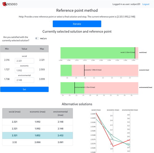
Figure 2. The UI for NIMBUS.

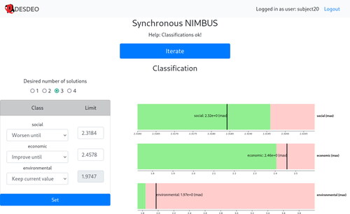
We offer two ways to specify preferences. The reference point in RPM can be set as numerical values in the form on the left in Figure 1, or by clicking on the bars on the right. Likewise, the classification for each objective in NIMBUS can be set manually by selecting classes and numerical values using the form on the left in Figure 2, or by clicking on the bars on the right, in which case the classification is inferred based on the value selected. Bars show currently set aspiration levels or bounds (vertical black lines) and current solution to be classified (lengths of pink bars). For RPM, pink bars represents currently selected solution. Additional method-specific controls are provided above the form. For NIMBUS, this means selecting the number of desired solutions to be calculated based on the classifications, and for RPM, specifying whether to stop the method or not. Moreover, the form and the bars are linked, i.e. changes in either are reflected in the other.

In RPM, below the form and bars, a table of solutions and a parallel coordinate plot enable selecting a solution (Figure 1). In NIMBUS, a similar table and a parallel coordinate plot are used to select a solution from previously computed ones; to select two solutions between which intermediate solutions are computed; to select previously computed solutions to be saved in an archive; and to select a preferred solution for classification or as the final solution. The table and the parallel coordinate plot are also linked.

Both UIs have a large blue button “Iterate” but the text changes depending on the context. For instance, in NIMBUS, the text is “Save” when solutions have been selected, and “Continue” when no solutions have been selected. The help text above the button is similarly dynamic, reflecting the current situation. If a method cannot continue, the blue button is disabled, and the help text provides a reason.

5.2. Participants and procedure

We recruited students and researchers as participants (N = 16). Half had a master’s, five a bachelor’s, and three a doctoral degree. One week before the experiment, we presented the sustainability problem and the interactive methods applied (see the Supplementary Material³). We also gave a 1-page summary of the problem to recall its details during the experiment.

A pilot study was conducted with the co-authors (one as an experimenter, one as an observer, two as participants) before the actual experiment to check the procedure and online environment (Zoom). The approximated length of the experiment was also then estimated. The experimenter first presented the informed consent and described the study. UIs were then demonstrated. All this took approximately 20 min.

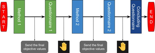
Next, the experimenter shared the Web address of the system introduced in Section 5.1 and credentials of the participants to log in. The experimenter and participants communicated via private chat. The same message templates were used to provide the necessary information without individual discussions. The method order was assigned at random: a half applied NIMBUS first, while the other half applied RPM. Each participant was given the name of the first method and the Web address of the related questionnaire. The participants were asked to solve the problem, send the objective values of their final solution, and fill out the first questionnaire. They were then asked to use “raise hand” button in Zoom, to get details of the second method.

The participants followed the same procedure for the second method. Finally, the experimenter provided the Web address of the concluding questionnaire. All participants completed it, i.e. they completed the experimental study. Figure 3 depicts the experiment procedure, which lasted approximately 60 min.

Figure 3. Procedure of the experiment.

5.3. Analysis and results

Next, we analyze quantitatively and qualitatively the participants’ responses to the items of Section 4. Our questionnaires used Webropol⁴. Participants used radio buttons for the Likert scale and semantic differential answers, and typed responses to open-ended questions in the text fields provided.

We applied Webropol’s internal statistical tools for average scores and standard deviations of the responses in the Likert scale and semantic differential and the Wilcoxon signed-rank test. The significance level was 0.05 for the p-values. Differences were statistically insignificant. Therefore, we do not report the p-values.

Textual data of the open-ended questions were analyzed with qualitative content analysis. A data-driven approach to qualitative content analysis (Weber, 1990) was conducted to identify semantic units and, through iterative analysis, create categories. The goal was to understand the reasons behind participants’ differences in the methods utilised.

Analyzing textual data with qualitative content analysis includes an in-depth reading of textual descriptions and numerous iterations to create content categories representing the data. Although qualitative content analysis can be laborious, it is beneficial when descriptions of participants’ experiences are needed. Textual data was important in understanding the reasons behind numerical Likert scale ratings and in concluding comparative items for a detailed understanding of why methods were preferred differently for different purposes and how participants acted as DMs. Next, we provide quantitative and qualitative findings answering research questions introduced in Section 4.1.

Cognitive load: As can be seen in Table 5, the responses to cognitive load were mostly similar for both methods. From the 1st item, NIMBUS required more mental activity (average = 4.88; standard deviaion (SD)=1.45) than RPM (average = 3.81; SD = 1.97). For finding the preferred solution (2nd item), the participants found RPM easier (average = 4.44; SD = 1.63) than NIMBUS (average = 4.00; SD = 1.59), which supports the results of the 1st item. Furthermore, the participants reported similar efforts (3rd item) for finding their preferred solutions, and frustration levels (4th item) were close to each other as well. Although they conducted a few more iterations with NIMBUS (based on the 5th item), tiredness was nearly the same (6th item).

Table 5. Responses as average scores for measuring cognitive load.

Questionnaire items	Average scores (SD)
	RPM	NIMBUS
1) A lot of mental activity was required (e.g. thinking, deciding, and remembering).	3.81 (1.97)	4.88 (1.45)
2) Finding the preferred solution was simple.	4.44 (1.63)	4.00 (1.59)
3) I had to work hard to find my preferred solution.	4.31 (1.49)	4.50 (1.59)
4) I felt frustrated in the solution process (e.g. insecure, discouraged, irritated, stressed).	3.31 (1.78)	3.56 (1.86)
5) It took too many iterations to arrive at an acceptable solution.	3.94 (1.57)	4.19 (1.68)
6) I felt tired.	2.63 (1.41)	2.75 (1.53)

Capturing preferences: Table 6 collects answers to capturing preferences. The scores and deviations of the easiness of providing preferences were the same for both methods (average = 6.00; SD = 1.03), indicating that the participants provided preferences easily. They could express preferences as they desired better in NIMBUS (average = 6.00; SD = 1.03) than in RPM (average = 5.31; SD = 1.14). Moreover, the participants learned to use RPM a bit more easily (average = 6.19; SD = 1.22) than NIMBUS (average = 5.88; SD = 1.15).

Table 6. Responses as average scores for capturing preferences.

Questionnaire items	Average scores (SD)
	RPM	NIMBUS
The preference information was easy to provide.	6.00 (1.03)	6.00 (1.03)
I was able to express my preferences as I wanted.	5.31 (1.14)	6.00 (1.03)
It was easy to learn to use this method.	6.19 (1.22)	5.88 (1.15)

Satisfaction: As can be seen in Table 7, the participants were satisfied with the final solution and convinced that it was the best one regardless of the method. Furthermore, with each method, they learned that the second and the third objectives conflict with each other.

Table 7. Responses as average scores for measuring satisfaction.

Questionnaire items	Average scores (SD)
	RPM	NIMBUS
I am satisfied with the final solution.	5.13 (1.09)	5.25 (1.00)
I think that the solution I found is the best one.	4.56 (1.15)	4.69 (1.35)
What degree of conflict do you think exists among each pair of objectives?:
Among f1 and f2	2.63 (1.09)	2.81 (1.22)
Among f1 and f3	2.44 (1.21)	2.13 (1.15)
Among f2 and f3	4.50 (0.73)	4.63 (0.81)

To assess satisfaction, an open-ended question was asked about why the solution process was terminated. The corresponding textual analyses are presented in Table 8. For both methods, not finding better solutions was the main reason to stop iterating. For NIMBUS, the sub-category of no further improvements was the main reason, and for RPM, it was the sub-category of maintaining the preferred objective values. Two participants also reported frustration with RPM that led them to stop, which was not the case with NIMBUS.

Table 8. Why did participants stop iterating?.

Why did you stop iterating?	NIMBUS (N = 16)	Example statements	RPM (N = 16)	Example statements
Compromise: no further improvements	n = 11	“I realised I could not achieve my overly optimistic results and stopped when found a decent compromise”.	n = 6	“I found the solution quite satisfactory for me and I am afraid the next solution is worse and I can’t go back”
Compromise: maintaining preferred objective	n = 4	“Was unable to further improve environmental objective without sacrificing the economic objective”.	n = 8	“I tried to improve the economic and environmental objectives and impair the social one but was not able to do it satisfactory so settled on this solution”.
Frustration	n = 0	–	n = 2	“The iteration felt like random generation that does not obey my reference point and I got frustrated”
Matching solution to previous method	n = 1	“I found a solution close to the solution I found with a previous method”	n = 0	–

Comparative questions: Analyzing comparative open-ended textual data followed the same procedure as the previous question. The responses are presented in Table 9.

Table 9. Results of the comparative items asked after completing both methods.

Questionnaire items	Number of participants (N = 16)
	RPM	NIMBUS
Which method was the easiest one to use?	9	7
Which method allowed you to learn most about the problem?	3	13
Which method would you like to use again?	3	13
Which solution do you like most?	6	10

RPM was regarded easier to use (n = 9) due to the easiness in providing preference information (5/9: e.g. “RPM is simple with just one type of input required. NIMBUS has a bit of a learning curve”) and simplicity of functionalities (2/9: “There is less functionality and choices with RPM and I feel it is easier to focus on trying new reference points because there are less steps (choices) between each iteration”).

On the other hand, the participants learned most about the problem with NIMBUS (n = 13). Preferring NIMBUS was due to the visibility of trade-offs and the possibility of saving solutions (5/13: e.g. “It was easier to see the trade-off and I didn’t have to think about the reference point that much so it was easier to focus on the solution process”) and due to an increasing understanding of the relations between the objectives (5/13: e.g. “It allowed me to explore the solutions in a more understandable way. As it has more options, I could compute similar solutions to the preferred one”). RPM was chosen by three participants due to simplicity (2/3: e.g. “Many ‘simple’ iterations — it felt like playing with the ‘knobs’. NIMBUS I got stuck and saw often solution sets narrowed down (many polylines were exactly the same) and I could not move it out of this zone”).

Almost all the participants (n = 13) stated NIMBUS as the method they wanted to use again. Preferring NIMBUS was based on functionalities (6/13), learnability (4/13), and interactivity (3/13). The main functionalities mentioned were a better way of setting preferences, an archive, and intermediate solutions (e.g. “In NIMBUS we can set view the archive of solutions and set preferences in a better way”). Learnability was described, e.g. as follows: “To know more about the conflict among the objectives of the problem”. The interactivity of NIMBUS was also considered a way to enhance the feeling of control.

The participants were also asked which final solution they liked most and why. Solutions with NIMBUS were preferred more (n = 10) than those of RPM (n = 6) due to the ability to follow preferences better with NIMBUS (3/10) and the feeling of control enabled by the functionalities of NIMBUS (7/10). The appreciated functionalities enabling to reach a desired solution with NIMBUS were the possibility of saving solutions for later comparison, finding intermediate solutions, and fine-tuning the solution (e.g. “Saving solutions for later comparison, more options for single objectives instead of just giving a ref.point”). Four participants preferred RPM solutions because of reaching more balanced and better solutions (4/6). RPM solutions were also preferred due to the possibility of maintaining desired values of pre-selected objectives (2/6). This revealed an anchoring effect, as the preferred solution with RPM was selected because it allowed participants to hold on to pre-decided trade-offs between objectives, favouring an objective over others.

Involvement of the participants as DMs: Finally, the participants were asked to respond to two items in Table 10. We wanted to ensure that they felt involved in acting as DMs while solving the problem. The overall credibility of the results depends on the participants’ understanding of the problem and perceived importance of solving it. Furthermore, to get reliable data, it is also important to design the experiment and present the problem engaging participants to act as real DMs.

Table 10. Responses as average scores on involvement levels of participants as DMs.

Questionnaire items	Average scores (SD)
The problem was easy to understand.	5.44 (1.41)
The problem was important for me to solve.	5.63 (0.96)

Overall, all participants understood the problem well and found it important to be solved (see Table 10). Three participants strongly agreed on understandability (e.g. “It was simple, and the objectives are understandable. I felt a connection and could imagine myself as a real DM”). A majority (n = 7) found the problem easy to understand due to few objective functions (e.g. “Even though the problem is very complex and demanding, the formulation that had only 3 objectives was simple enough to understand and work with”). Three participants considered the problem somewhat understandable, but the objective values seemed abstract due to compound objectives (e.g. “The problem is fairly understandable, but because of the compound objectives it is bit hard to interpret what does it mean to decrease value of the social objective function”). Lower scores (neither agree nor disagree (n = 1), somewhat disagree (n = 1), and disagree (n = 1)) were only selected by three participants.

Nine participants found the problem important due to its timeliness and essentiality (e.g. “I felt a connection to the problem and wanted to compare the trade-offs and find the most preferred one to me as a DM to find a sustainable solution”). Participants who felt strongly about the importance (n = 2) were concerned about our future, and on the other hand, participants who had no firm opinion (neither agree nor disagree, n = 3), commented that the government should address decisions concerning sustainability (n = 1), or the problem was not something they think of (n = 1).

6. Discussion

As mentioned in the introduction, our aim was to provide realistic means of comparing interactive methods from the aspects of cognitive load, capturing preferences, and DM’s satisfaction. Next, we discuss our experimental results and the limitations of the study design and analysis.

As demonstrated in Section 5.3, our results reveal that quantitative and qualitative analyses serve various purposes. The responses to items asked after using each method were nearly identical for both methods. While there was no apparent winner based on the quantitative analysis, the opinion on the preferred methods became clearer after they had used both methods.

NIMBUS was found cognitively more demanding based on the quantitative analysis while the participants found RPM easier to use. However, when asked which method they would use again, most participants (n = 13) chose NIMBUS. Although they found RPM easy to learn and simple to use, they thought NIMBUS allowed gaining more insights about the problem as it provides more functionalities enabling capturing preferences better. We can conclude that NIMBUS responded better to the provided preferences, which positively affected the participants’ learning about the problem.

The participants were satisfied with the final solution found using both methods and believed it was the best they could find. This means they were able to find a satisfactory balance between objectives. Most of them (n = 10) preferred the NIMBUS solution. As mentioned, NIMBUS offers more functionalities allowing the participants to feel in control and provide preferences more effectively, which may help reach a satisfactory solution.

Overall, the participants found the problem understandable and important since its objectives had real meanings. We emphasize that the relevance of the problem and its description are crucial to get reliable data, since it makes the participants take the experiment seriously and act as real DMs. In this, questions about participants’ involvement as DMs could capture the issues. Therefore, it is recommended to include these questions to validate the participants’ understanding of the problem and their involvement in solving it.

A within-subjects design allowed asking comparative open-ended questions and comparing satisfaction with the final solutions of different methods. But we had to limit the number of questionnaire items since the participants used both methods. It is important to avoid tiring participants with excessive amounts of questions per method. Having a too laborious experiment for the participants affects the quality and reliability of the results.

If a higher number of interactive methods is to be compared, a between-subject design with more participants is justifiable (even though comparing the abovementioned satisfaction will not be possible). A between-subject design may also allow assessing more aspects because participants only use one method, allowing more questions to be asked. Although this experiment was a proof of concept, our questionnaire design offers possibilities for further research towards investigating more aspects of interactive methods and considering different cognitive biases affecting interactive solution processes.

As in any experiment, also this study has limitations. One of them is the number of participants. It was a conscious choice because of the proof of concept nature. However, we considered the diversity of our participants’ educational degrees, and they all were instructed on the basics of the interactive methods and the problem. Having a limited number of participants could be one of the reasons why the quantitative results were not statistically significant.

7. Conclusions

We have proposed an experimental design and a questionnaire to compare interactive methods in cognitive load, capturing preferences, and DM’s satisfaction. Unlike earlier publications, our approach is reproducible with sufficient information so that experiments can be conducted to compare different methods.

We conducted an experiment and analyzed the results to show the applicability of the proposed questionnaire and design as proof of concept. The proposed questionnaire and design allowed us to compare several crucial aspects of interactive methods. We shared details to make this experiment reusable, reproducible, and extendable.

This is the initial step in a more extensive research agenda to identify ways to compare interactive methods. We plan future studies with more participants and extended questionnaires to assess additional aspects of interactive methods. Furthermore, the questionnaire items could be developed into validated measurements. Existing validated measurements are here inapplicable, as stated before. Therefore, further studies are needed.

Acknowledgements

We thank Professor Theodor Stewart for helpful comments. This research was partly supported by the Academy of Finland (grants 311877 and 322221) and the Vilho, Yrjö and Kalle Väisälä Foundation (grant 200033) and is related to the thematic research area DEMO (Decision Analytics utilizing Causal Models and Multiobjective Optimization, jyu.fi/demo) at the University of Jyvaskyla; the Spanish Ministry of Science (projects PID2019-104263RB-C42 and PID2020-115429GB-I00); the Regional Government of Andalucía (projects SEJ-532, P18-RT-1566 and UMA18-FEDERJA-065); and the University of Málaga (grant B1-2020-18).

Disclosure statement

No potential conflict of interest was reported by the authors.

Notes

1 https://ec.europa.eu/eurostat/web/sdi/main-tables

2 https://nextcloud.jyu.fi/index.php/s/KLJ4o6WLgABdWTJ

3 http://www.mit.jyu.fi/optgroup/extramaterial.html#2021-1

4 https://webropol.com/

References

- Afsar, B., Miettinen, K., & Ruiz, A. B. (2021a). An artificial decision maker for comparing reference point based interactive evolutionary multiobjective optimization methods. In H. Ishibuchi (Eds.), Evolutionary multi-criterion optimization, 11th International Conference, EMO 2021, Proceedings (pp. 619–631). Springer.
- Afsar, B., Miettinen, K., & Ruiz, F. (2021b). Assessing the performance of interactive multiobjective optimization methods: A survey. ACM Computing Surveys, 54(4):85, 1–27. https://doi.org/10.1145/3448301
- Afsar, B., Ruiz, A. B., & Miettinen, K. (2021). Comparing interactive evolutionary multiobjective optimization methods with an artificial decision maker. Complex & Intelligent Systems. https://doi.org/10.1007/s40747-021-00586-5
- Battiti, R., & Passerini, A. (2010). Brain-computer evolutionary multiobjective optimization: A genetic algorithm adapting to the decision maker. IEEE Transactions on Evolutionary Computation, 14(5), 671–687. https://doi.org/10.1109/TEVC.2010.2058118
- Brockhoff, K. (1985). Experimental test of MCDM algorithms in a modular approach. European Journal of Operational Research, 22(2), 159–166. https://doi.org/10.1016/0377-2217(85)90224-3
- Buchanan, J. T. (1994). An experimental evaluation of interactive MCDM methods and the decision making process. Journal of the Operational Research Society, 45(9), 1050–1059. https://doi.org/10.1057/jors.1994.170
- Buchanan, J. T., & Corner, J. (1997). The effects of anchoring in interactive MCDM solution methods. Computers & Operations Research, 24(10), 907–918. https://doi.org/10.1016/S0305-0548(97)00014-2
- Buchanan, J. T., & Daellenbach, H. G. (1987). A comparative evaluation of interactive solution methods for multiple objective decision models. European Journal of Operational Research, 29(3), 353–359. https://doi.org/10.1016/0377-2217(87)90248-7
- Chen, L., Xin, B., & Chen, J. (2017). A tradeoff-based interactive multi-objective optimization method driven by evolutionary algorithms. Journal of Advanced Computational Intelligence and Intelligent Informatics, 21(2), 284–292. https://doi.org/10.20965/jaciii.2017.p0284
- Cook, T. D., & Campbell, D. T. (1979). Quasi-experimentation: Design and analysis issues for field settings. Houghton Mifflin Company.
- Hart, S. G. (2006). NASA-task load index (NASA-TLX); 20 years later. In Proceedings of the Human Factors and Ergonomics Society Annual Meeting, 50(9), 904–908. https://doi.org/10.1177/154193120605000909
- Hart, S. G., & Staveland, L. E. (1988). Development of NASA-TLX (task load index): Results of empirical and theoretical research. In Advances in psychology (Vol. 52, pp. 139–183). Elsevier.
- Huber, S., Geiger, M. J., & Sevaux, M. (2015). Simulation of preference information in an interactive reference point-based method for the bi-objective inventory routing problem. Journal of Multi-Criteria Decision Analysis, 22(1–2), 17–35. https://doi.org/10.1002/mcda.1534
- Hwang, C.-L., & Masud, A. (1979). Multiple objective decision making – Methods and applications: A state-of-the-art survey. Springer.
- Joshi, A., Kale, S., Chandel, S., & Pal, D. K. (2015). Likert scale: Explored and explained. British Journal of Applied Science & Technology, 7(4), 396–403. https://doi.org/10.9734/BJAST/2015/14975
- Kok, M. (1986). The interface with decision makers and some experimental results in interactive multiple objective programming methods. European Journal of Operational Research, 26(1), 96–107. https://doi.org/10.1016/0377-2217(86)90162-1
- Korhonen, P., & Wallenius, J. (1989). Observations regarding choice behaviour in interactive multiple criteria decision-making environments: An experimental investigation. In A. Lewandowski & I. Stanchev (Eds.), Methodology and software for interactive decision support (pp. 163–170). Springer.
- Likert, R. (1932). A technique for the measurement of attitudes. Archives of Psychology, 22(140), 5–55.
- López-Ibáñez, M., & Knowles, J. (2015). Machine decision makers as a laboratory for interactive EMO. In A. Gaspar-Cunha, C. Henggeler Antunes, & C. C. Coello (Eds.), Evolutionary multi-criterion optimization, 8th International Conference, Proceedings, Part II (pp. 295–309). Springer.
- López-Jaimes, A., & Coello, C. A. (2014). Including preferences into a multiobjective evolutionary algorithm to deal with many-objective engineering optimization problems. Information Sciences, 277, 1–20. https://doi.org/10.1016/j.ins.2014.04.023
- Luque, M., Ruiz, F., & Miettinen, K. (2011). Global formulation for interactive multiobjective optimization. Or Spectrum, 33(1), 27–48. https://doi.org/10.1007/s00291-008-0154-3
- Miettinen, K. (1999). Nonlinear multiobjective optimization. Kluwer Academic Publishers.
- Miettinen, K., Hakanen, J., & Podkopaev, D. (2016). Interactive nonlinear multiobjective optimization methods. In S. Greco, M. Ehrgott, & J. Figueira (Eds.), Multiple criteria decision analysis: State of the art surveys (Vol. 2, pp. 931–980). Springer.
- Miettinen, K., & Mäkelä, M. (2006). Synchronous approach in interactive multiobjective optimization. European Journal of Operational Research, 170(3), 909–922. https://doi.org/10.1016/j.ejor.2004.07.052
- Miettinen, K., Ruiz, F., & Wierzbicki, A. P. (2008). Introduction to multiobjective optimization: Interactive approaches. In J. Branke, K. Deb, K. Miettinen, & R. Słowiński (Eds.), Multiobjective optimization: Interactive and evolutionary approaches (pp. 27–57). Springer.
- Misitano, G., Saini, B. S., Afsar, B., Shavazipour, B., & Miettinen, K. (2021). DESDEO: The modular and open source framework for interactive multiobjective optimization. IEEE Access, 9, 148277–148295. https://doi.org/10.1109/ACCESS.2021.3123825
- Narasimhan, R., & Vickery, S. K. (1988). An experimental evaluation of articulation of preferences in multiple criterion decision-making (MCDM) methods. Decision Sciences, 19(4), 880–888. https://doi.org/10.1111/j.1540-5915.1988.tb00309.x
- Narukawa, K., Setoguchi, Y., Tanigaki, Y., Olhofer, M., Sendhoff, B., & Ishibuchi, H. (2016). Preference representation using Gaussian functions on a hyperplane in evolutionary multi-objective optimization. Soft Computing, 20(7), 2733–2757. https://doi.org/10.1007/s00500-015-1674-9
- Podkopaev, D., Miettinen, K., & Ojalehto, V. (2021). An approach to the automatic comparison of reference point-based interactive methods for multiobjective optimization. IEEE Access, 9, 150037–150048. https://doi.org/10.1109/ACCESS.2021.3123432
- Ricciolini, E., Rocchi, L., Cardinali, M., Paolotti, L., Ruiz, F., Cabello, J. M., & Boggia, A. (2022). Assessing progress towards SDGs implementation using multiple reference point based multicriteria methods: The case study of the European countries. Social Indicators Research, 162(3), 1233–1260. https://doi.org/10.1007/s11205-022-02886-w
- Ruiz, F., Luque, M., & Miettinen, K. (2012). Improving the computational efficiency in a global formulation (GLIDE) for interactive multiobjective optimization. Annals of Operations Research, 197(1), 47–70. https://doi.org/10.1007/s10479-010-0831-x
- Saisana, M., & Philippas, D. (2012). Sustainable society index (SII): Taking societies’ pulse along social, environmental and economic issues. The Joint Research Centre audit on the SSI (Vol. JRC76108; Tech. Rep.) Publications Office of the European Union.
- Sinha, A., Korhonen, P., Wallenius, J., & Deb, K. (2010). An interactive evolutionary multi-objective optimization method based on polyhedral cones. In C. Blum & R. Battiti (Eds.), Learning and intelligent optimization (pp. 318–332). Springer.
- Stewart, T. J. (2005). Goal programming and cognitive biases in decision-making. Journal of the Operational Research Society, 56(10), 1166–1175. https://doi.org/10.1057/palgrave.jors.2601948
- Tversky, A., & Kahneman, D. (1974). Judgment under uncertainty: Heuristics and biases. Science (New York, N.Y.), 185(4157), 1124–1131.
- United Nations. (2015). Transforming our world: The 2030 agenda for sustainable development. https://sustainabledevelopment.un.org/post2015/transformingourworld
- Wallenius, J. (1975). Comparative evaluation of some interactive approaches to multicriterion optimization. Management Science, 21(12), 1387–1396. https://doi.org/10.1287/mnsc.21.12.1387
- Weber, R. P. (1990). Basic content analysis. Sage.
- Wierzbicki, A. P. (1980). The use of reference objectives in multiobjective optimization. In G. Fandel & T. Gal (Eds.), Multiple criteria decision making, theory and applications (pp. 468–486). Springer.