Goal programming duality revisited: Formulation of a set of variant duals

Abstract

The formulation of the duals of the original goal programming variants took place in the decades following its introduction, principally for computational purposes. However the development of more recent Goal Programming variants has not been matched by the formulation and analysis of their associated duals. This paper furthers the topic of goal programming duality by formulating the duals of a progressive sequence of up to the most recent Goal Programming models: Weighted, Chebyshev, Extended and Extended Network Goal Programming models. It interprets the results and shows the insights that the duals can provide, principally by providing an understanding of the interactions between the multiple objectives in each case. The paper concludes with a comparison of the results and shows how the sequence of duals mirrors the sequence of the associated primals.

Keywords:

• Goal programming
• duality
• multiple criteria decision making

1. Introduction

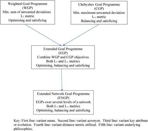
The concept of Goal Programming (GP) - that is, the minimisation in some sense of the unwanted deviations from a set of desirable, decision-maker-set goals - was first introduced for a specific application by Charnes et al. (1955) and later expanded by Charnes and Cooper as a more general theory (1961). The original goal programming models were based on the minimisation of an L₁ distance of the unwanted deviations from the goals, whether in a pre-emptive (lexicographic) or non-pre-emptive (weighted) form. A series of variants of the Goal Programming model has been formulated in the intervening decades to allow more accurate modelling of the decision makers’ preferences via the incorporation of different underlying philosophies (Jones & Oliveira, 2022). The Chebyshev goal programming variant (CGP) was introduced by Flavell (1976) to allow for the consideration of the $L_{\infty }$ distance, representing balance between goals. The extended goal programming variant (EGP - Romero, 2001) introduces a parametric mix of L₁ and $L_{\infty }$ distances, and hence optimises a parametrically controlled mix of efficiency and balance. Jones et al. (2016) expand the extended goal programming to consider centralisation, balance between objectives and balance between stakeholders over a multi-objective, multi-stakeholder network, termed extended network goal programming (ENGP). There are also other variants, the most recent including Multi-choice GP (Chang, 2007), Revised Multi-choice GP (Chang, 2007a and Paksoy & Chang, 2010) and Meta-goal programming (Uria et al., 2002). However the WGP, CGP, EGP and ENGP variants form a key sequence because they take the two fundamental models - the L₁ WGP and the $L_{\infty }$ CGP - and combine them first in the EGP variant and then the ENGP variant. This developmental relationship is shown in Figure 1. A recent mapping of goal programming variants can be be found in Jones and Romero (2019).

Figure 1. Goal programming variant evolution.

The early goal programming variants tended to use the lexicographic variant, with solution as a series of linear or integer programming models, dependent on the presence of discrete decision variables or not (Ignizio, 1976). The earliest goal programming dual models were hence formulated in the context of enhanced lexicographic solution, for instance Markowski and Ignizio (1983) and Ignizio (1985) present a multi-dimensional dual solution methodology for the lexicographic variants which allows more rapid solution than the augmentation solution methods used prior to this advance. Ogryczak (1988) presents an alternative lexicographic dual, with the property that the dual of the dual is the primal. Pourkarimi and Zarepisheh (2007) present a dual-based solution for a more general class of of lexicographic multiple objective programmes, concentrating on the solution-enhancing aspects of the dual formulation.

The recent trend in goal programming is towards non-pre-emptive models, due to their enhanced preferential flexibility and exploration of trade-offs (Jones & Oliveira, 2022). Recent examples, for instance, are in Healthcare (Arik et al., 2020; Razavi et al., 2021; Wang, 2019) and in security (Dillenburger et al., 2019). Gong et al. ( 2020) formulate the dual of a type of weighted goal programme for group decision-making with interval judgements, and draw some economic conclusions regarding the compensation required for consensus. This result has given rise to a considerable work in the field of group decision making, with Wang and Wu (2021), Zhang et al. (2020), Gong et al. (2020) and Chao et al. (2022) providing recent contributions.

However, there remain significant gaps in the formulation of the duals of the non-pre-emptive goal programming variants, with no dual formulations for recent variants available to date. As detailed above, the work of Gong et al. (2020) looked at duality in a specific context. Apart from this example there has been a dearth of exploration of the meaning of the duals for goal programming modelling and the interpretation of results. This paper aims to fill these research gaps by:

1. Developing the duals of the key sequence of non-pre-emptive goal programming variants described in Figure 1: WGP; CGP; EGP and ENGP.

2. Demonstrating linkages beween the four formulated variant duals.

3. Providing the basis for further research that will give economic and modelling insight into the significance of the key extended GP variant dual by examination of its duality properties.

The remainder of this paper is divided into four sections. Section 2 formulates the WGP, CGP, EGP and ENGP dual models; Section 3 demonstrates the linkages between them; and Section 4 provides a summary and outlines some possible further analysis.

2. Goal programming variant duals

A generic Goal Programme (Jones & Tamiz, 2010) may be represented as:

Minimise (1) $$a=h(\mathbf{n},\mathbf{p})$$(1)

Subject to: (2) $$f_q(\mathbf{x})+{\mathrm{n}}_{\mathrm{q}}-{\mathrm{p}}_{\mathrm{q}}=b_q q=1,\dots ,Q$$(2) (3) $$\mathbf{x} \epsilon R$$(3) (4) $$n_q, p_q\ge 0 q=1,\dots ,Q.$$(4)

The generic Goal Programme has Q goals involving n decision variables $\mathbf{x}={\mathrm{x}}_1,{\mathrm{x}}_2,\dots ,{\mathrm{x}}_{\mathrm{n}}.$ Each goal q has a target value b_q and an achieved value $f_q(x).$ Each goal then has positive or negative deviational variables p_q and n_q respectively. p_q and n_q are non-negative and cannot both be non-zero simultaneously. h is a function of the deviational variables representing the penalties associated with non-achievement of the targets and R is the feasible region of x in decision space.

A number of variants of the generic model have been developed since the inception of goal programming. This paper derives the duals of a number of these variants that form a logical sequence of increasing complexity. The relationship between these variants is shown in Figure 1.

2.1. Weighted Goal Programming

In Weighted Goal Programming (WGP) the objective function provides a straightforward sum of the deviational variables by allocating suitable weights to each of them (the L₁ metric). Jones and Tamiz (2010) recommend normalising the weights and so, using percentage normalisation and assuming that $b_q>0q=1,\dots ,Q,$ the model becomes:

Minimise (5) $$a=\sum _{q=1}^Q(\frac{u_q{n}_q}{b_q}+\frac{v_q{p}_q}{b_q})$$(5)

Subject to: (6) $$f_q(\mathbf{x})+{\mathrm{n}}_{\mathrm{q}}-{\mathrm{p}}_{\mathrm{q}}=b_q q=1,\dots ,Q$$(6) (7) $$\mathbf{x} \epsilon R$$(7) (8) $$n_q, p_q\ge 0 q=1,\dots ,Q.$$(8) where R is the feasible region of x in decision space.

The relative simplicity of the model has led to its application in a variety of fields (see for example Ruben et al. (2020) and Omrani et al. (2019)). For simplicity, and without loss of generality, we now omit the subsidiary equations resulting from the condition $\mathbf{x}ϵ$ R apart from the requirement that $\mathbf{x}\ge 0.$

Using Equations (5)–(8)(8) $$n_q, p_q\ge 0 q=1,\dots ,Q.$$(8) and letting $c_q=\frac{u_q}{b_q}$ and ${\widehat{\mathrm{c}}}_{\mathrm{q}}=\frac{v_q}{b_q}$ we define ${\mathbf{C}}^{\mathbf{T}}=[{\mathrm{c}}_1, {\mathrm{c}}_2, \dots ,{\mathrm{c}}_{\mathrm{Q}}]$ and ${\widehat{\mathbf{C}}}^{\mathbf{T}}=[{\widehat{\mathrm{c}}}_1, {\widehat{\mathrm{c}}}_2, \dots ,{\widehat{\mathrm{c}}}_{\mathrm{Q}}].$ Furthermore let $\mathbf{F}(x)=[{\mathrm{f}}_1(\mathbf{x}),{\mathrm{f}}_2(\mathbf{x}), \dots , {\mathrm{f}}_{\mathrm{Q}}(\mathbf{x})],$ ${\mathbf{n}}^{\mathbf{T}}=[{\mathrm{n}}_1,{\mathrm{n}}_2,\dots ,{\mathrm{n}}_{\mathrm{Q}}],{\mathbf{p}}^{\mathbf{T}}=[{\mathrm{p}}_1,{\mathrm{p}}_2,\dots ,{\mathrm{p}}_{\mathrm{Q}}]$ and ${\mathbf{b}}^{\mathbf{T}}=[{\mathrm{b}}_1, {\mathrm{b}}_2, \dots , {\mathrm{b}}_{\mathrm{Q}}].$ Then the general model can be re-written as:

Minimise: (9) $$a=\left[\begin{array}{ccc}\mathbf{0}& {\mathbf{C}}^{\mathbf{T}}& {\widehat{\mathbf{C}}}^{\mathbf{T}}\end{array}\right]\left[\begin{array}{c}\mathbf{x}\\ \mathbf{n}\\ \mathbf{p}\end{array}\right]$$(9)

Subject to: (10) $$\left[\begin{array}{ccc}\mathbf{F}& \mathbf{I}& -\mathbf{I}\end{array}\right]\left[\begin{array}{c}\mathbf{x}\\ \mathbf{n}\\ \mathbf{p}\end{array}\right]=\mathbf{b}$$(10) (11) $$\hspace{1em}\mathbf{x},\mathbf{n},\mathbf{p}\ge 0$$(11) where $\mathbf{I}$ is a suitably dimensioned identity matrix.

If ${\mathbf{w}}^{\mathbf{T}}=[{\mathrm{w}}_1,{\mathrm{w}}_2,\dots ,{\mathrm{w}}_{\mathrm{Q}}]$ then the dual of the primal problem is:

Maximise: (12) $$a={\mathbf{b}}^{\mathbf{T}}\mathbf{w}$$(12)

Subject to: (13) $$\left[\begin{array}{c}{\mathbf{F}}^{\mathbf{T}}\hfill \\ \mathbf{I}\hfill \\ -\mathbf{I}\hfill \end{array}\right]\left[\begin{array}{c}\mathbf{w}\\ \widehat{\mathbf{w}}\end{array}\right]\le \left[\begin{array}{c}\mathbf{0}\\ \mathbf{C}\\ \widehat{\mathbf{C}}\end{array}\right]$$(13) $\mathbf{w}$ is unconstrained.

This implies that: (14) $${\mathbf{F}}^{\mathbf{T}}\mathbf{w}\le \mathbf{0}$$(14) (15) $$-\widehat{\mathbf{C}}\le \mathbf{w}\le \mathbf{C}$$(15)

2.2. Chebyshev Goal Programming

In Chebyshev Goal Programming (CGP) the objective is to minimise the maximum deviation for any goal. This was first used by Flavell (1976) but more recent examples are given in, for example, Despotis and Derpanis (2008) and Ho (2019). This” minimax” criterion therefore uses the $L_{\infty }$ metric and aims to achieve a balance between the different levels of satisfaction of each of the goals. The model is then:

Minimise: (16) $$a=D$$(16)

Subject to: (17) $$f_q(\mathbf{x})+{\mathrm{n}}_{\mathrm{q}}-{\mathrm{p}}_{\mathrm{q}}=b_q q=1,\dots ,Q$$(17) (18) $$\frac{u_q{n}_q}{b_q}+\frac{v_q{p}_q}{b_q}\le D q=1,\dots ,Q$$(18) (19) $$\mathbf{x} \epsilon F$$(19) (20) $$n_q, p_q\ge 0 q=1,\dots ,Q.$$(20) (21) $$D\ge 0$$(21)

All variables non-negative.

With:

$\mathbf{G}$ being the diagonal matrix with diagonal term $c_i\hspace{1em}i=1,\dots ,Q$

$\widehat{\mathbf{G}}$ being the diagonal matrix with diagonal term ${\widehat{c}}_i\hspace{1em}i=1,\dots ,Q$

then, using the same notation as before, the model becomes:

Minimise: (22) $$a=\left[\begin{array}{cccc}\mathbf{0}& \mathbf{0}& \mathbf{0}& 1\end{array}\right]{\left[\begin{array}{cccc}\mathbf{x}& \mathbf{n}& \mathbf{p}& D\end{array}\right]}^T$$(22)

Subject to: (23) $$\left[\begin{array}{cccc}\mathbf{F}& \mathbf{I}& -\mathbf{I}& \mathbf{0}\\ \mathbf{0}& \mathbf{G}& \widehat{\mathbf{G}}& -\widehat{\mathbf{I}}\end{array}\right]\left[\begin{array}{c}\mathbf{x}\\ \mathbf{n}\\ \mathbf{p}\\ D\end{array}\right]=\left[\begin{array}{c}\mathbf{b}\hfill \\ \mathbf{0}\hfill \end{array}\right]\hspace{1em}\mathbf{x},\mathbf{n},\mathbf{p},\mathrm{D}\ge 0$$(23) where $\widehat{\mathbf{I}}=[1,1,\dots ,1].$

If ${\mathit{\gamma }}^T=[{\gamma }_1,{\gamma }_2,\dots ,{\gamma }_Q]$ then the dual of the primal problem is:

Maximise: (24) $$a=\left[\begin{array}{cc}{\mathbf{b}}^{\mathbf{T}}& \mathbf{0}\end{array}\right]\left[\begin{array}{c}\mathbf{w}\\ \mathit{\gamma }\end{array}\right]$$(24)

Subject to: (25) $$\left[\begin{array}{cc}{\mathbf{F}}^{\mathbf{T}}& \mathbf{0}\\ \mathbf{I}& \mathbf{G}\\ -\mathbf{I}& \widehat{\mathbf{G}}\\ \mathbf{0}& -{\widehat{\mathbf{I}}}^{\mathbf{T}}\end{array}\right]\left[\begin{array}{c}\mathbf{w}\\ \mathit{\gamma }\end{array}\right]\le \left[\begin{array}{c}\mathbf{0}\\ \mathbf{0}\\ \mathbf{0}\\ 1\end{array}\right]$$(25) $\mathbf{w}$ is unrestricted; $\mathit{\gamma }\le 0.$

This implies that: (26) $$\begin{array}{c}{\mathbf{F}}^{\mathbf{T}}\mathbf{w}\le \mathbf{0}\\ \mathit{\gamma }\widehat{\mathbf{G}}\le \mathbf{w}\le -\mathit{\gamma }\mathbf{G}\hspace{1em}\Rightarrow \hspace{1em}-{\mathrm{c}}_{\mathrm{q}}\le \frac{{\mathrm{w}}_{\mathrm{q}}}{{\gamma }_{\mathrm{q}}}\le {\widehat{c}}_{\mathrm{q}}\end{array}$$(26) (27) $$-{\widehat{\mathbf{I}}}^{\mathbf{T}}\mathit{\gamma }\le 1\hspace{1em}\Rightarrow \hspace{1em}\sum _{\mathrm{q}}{\gamma }_{\mathrm{q}}\ge -1$$(27)

Equation (27)(27) $$-{\widehat{\mathbf{I}}}^{\mathbf{T}}\mathit{\gamma }\le 1\hspace{1em}\Rightarrow \hspace{1em}\sum _{\mathrm{q}}{\gamma }_{\mathrm{q}}\ge -1$$(27) also means that: (28) $$-1\le \sum _q{\gamma }_q\le 0.$$(28)

2.3. Extended Goal Programming

Extended Goal Programming (EGP) was first suggested by Romero (2001) in the context of a lexicographic ordering of the goals and was later generalised in Romero (2004). More recent applications include Guijarro et al. (2018) and Pal and Kumar (2014). It aims to allow both of the above approaches by combining the optimising given by WGP with the balancing given by CGP. For a non-lexicographic EGP the general model is:

Minimise: (29) $$a=\alpha D+(1-\alpha )\sum _{q=1}^Q(\frac{u_q{n}_q}{b_q}+\frac{v_q{p}_q}{b_q})$$(29)

Subject to: (30) $$f_q(\mathbf{x})+{\mathrm{n}}_{\mathrm{q}}-{\mathrm{p}}_{\mathrm{q}}=b_q q=1,\dots ,Q$$(30) (31) $$\frac{u_q{n}_q}{b_q}+\frac{v_q{p}_q}{b_q}\le D q=1,\dots ,Q$$(31) (32) $$\mathbf{x} \epsilon F$$(32) (33) $$n_q, p_q\ge 0 q=1,\dots ,Q$$(33) (34) $$D\ge 0.$$(34)

The parameter α is a constant between 0 and 1 which controls the mix of optimisation (L₁) and balance ($L_{\infty }$) in the achievement function. The general model for an EGP given in Equations (29)–(34)(34) $$D\ge 0.$$(34) can be expressed in matrix terms as:

Minimise: (35) $$a=\left[\begin{array}{cccc}\mathbf{0}& (1-\alpha )\mathbf{C}& (1-\alpha )\widehat{\mathbf{C}}& \alpha \end{array}\right]{\left[\begin{array}{cccc}\mathbf{x}& \mathbf{n}& \mathbf{p}& D\end{array}\right]}^T$$(35)

Subject to: (36) $$\left[\begin{array}{cccc}\mathbf{F}& \mathbf{I}& -\mathbf{I}& \mathbf{0}\\ \mathbf{0}& \mathbf{G}& \widehat{\mathbf{G}}& -\widehat{\mathbf{I}}\end{array}\right]\left[\begin{array}{c}\mathbf{x}\\ \mathbf{n}\\ \mathbf{p}\\ \mathrm{D}\end{array}\right]=\left[\begin{array}{c}\mathbf{b}\\ \mathbf{0}\end{array}\right]$$(36)

All variables non-negative.

The dual of the primal problem is then:

Maximise: (37) $$a=\left[\begin{array}{cc}{\mathbf{b}}^{\mathbf{T}}& \mathbf{0}\end{array}\right]\left[\begin{array}{c}\mathbf{w}\\ \mathit{\gamma }\end{array}\right]$$(37)

Subject to: (38) $$\left[\begin{array}{cc}{\mathbf{F}}^{\mathbf{T}}& \mathbf{0}\\ \mathbf{I}& \mathbf{G}\\ -\mathbf{I}& \widehat{\mathbf{G}}\\ \mathbf{0}& -{\widehat{\mathbf{I}}}^{\mathbf{T}}\end{array}\right]\left[\begin{array}{c}\mathbf{w}\\ \mathit{\gamma }\end{array}\right]\le \left[\begin{array}{c}\mathbf{0}\\ (1-\alpha )\mathbf{C}\\ (1-\alpha )\widehat{\mathbf{C}}\\ \alpha \end{array}\right]$$(38) $\mathbf{w}$ is unrestricted, $\mathit{\gamma }\le \mathbf{0}.$

This implies that: (39) $${\mathbf{F}}^{\mathbf{T}}\mathbf{w}\le \mathbf{0}$$(39) (40) $$\widehat{\mathbf{G}}\mathit{\gamma }-\widehat{\mathbf{C}}(1-\alpha )\le \mathbf{w}\le -\mathbf{G}\mathit{\gamma }+\mathbf{C}(1-\alpha )$$(40) (41) $$\Rightarrow -{\mathrm{c}}_{\mathrm{q}}\le \frac{w_q}{[{\gamma }_q-(1-\alpha )]}\le {\widehat{c}}_q$$(41) (42) $$-{\widehat{\mathbf{I}}}^{\mathbf{T}}\mathit{\gamma }\le \alpha$$(42) (43) $$\hspace{1em}\Rightarrow \sum _{q=1}^Q{\gamma }_q\ge -\alpha$$(43)

Hence, similarly to the CGP model, Equation (43)(43) $$\hspace{1em}\Rightarrow \sum _{q=1}^Q{\gamma }_q\ge -\alpha$$(43) can be written as: (44) $$-\alpha \le \sum _{q=1}^Q{\gamma }_q\le 0.$$(44)

2.4. Extended Network Goal Programming

A recent extension of these ideas, known as Extended Network Goal Programming (ENGP), allows for a weighted combination of EGPs that might represent, for example, the relative needs of a network of stakeholders. Jones et al. (2016) describe the ENGP model as:

Minimise: (45) $$\begin{array}{c}a=W_1\left[{\alpha }^{(j^1)}{\lambda }^{(j^1)}+(1-{\alpha }^{(j^1)})\sum _{k=1}^K\left(\frac{u_k^{(j^1)}{n}_k^{(j^1)}}{b_k^{(j^1)}}+\frac{v_k^{(j^1)}{p}_k^{(j^1)}}{b_k^{(j^1)}}\right)\right]\\ +\sum _{l=2}^L{W}_l\left[{\beta }_l{D}_l+(1-{\beta }_l)\sum _{j^l=1}^{J^l}\left\{({\alpha }^{(j^l)}{\lambda }^{(j^l)}+(1-{\alpha }^{(j^l)})\sum _{k=1}^K\left(\frac{u_k^{(j^l)}{n}_k^{(j^l)}}{b_k^{(j^l)}}+\frac{v_k^{(j^l)}{p}_k^{(j^l)}}{b_k^{(j^l)}}\right)\right\}\right]\end{array}$$(45) subject to: (46) $$\begin{array}{c}{f}_k^{(j^l)}(\mathbf{x})+{\mathrm{n}}_{\mathrm{k}}^{{\mathrm{(}\mathrm{j}}^{\mathrm{l}}\mathrm{)}}-{\mathrm{p}}_{\mathrm{k}}^{{\mathrm{(}\mathrm{j}}^{\mathrm{l}}\mathrm{)}}=b_k^{(j^l)}\\ k=1,\dots ,K;\hspace{1em}{j}^l=1,\dots ,J^l;\hspace{1em}l=1,\dots ,L.\end{array}$$(46) (47) $$\begin{array}{c}\frac{u_k^{(j^l)}{n}_k^{(j^l)}}{b_k^{(j^l)}}+\frac{v_k^{(j^l)}{p}_k^{(j^l)}}{b_k^{(j^l)}}\le {\lambda }^{(j^l)}\\ k=1,\dots ,K;\hspace{1em}{j}^l=1,\dots ,J^l;\hspace{1em}l=1,\dots ,L.\end{array}$$(47) (48) $${\alpha }^{j^l}{\lambda }^{(j^l)}+(1-{\alpha }^{(j^l)})\sum _{k=1}^K\left(\frac{u_k^{(j^l)}{n}_k^{(j^l)}}{b_k^{(j^l)}}+\frac{v_k^{(j^l)}{p}_k^{(j^l)}}{b_k^{(j^l)}}\right)\le D_l\hspace{1em}{j}^l=2,\dots ,J^l;\hspace{1em}l=2,\dots ,L$$(48) (49) $$\mathbf{x}\epsilon F$$(49) (50) $$\begin{array}{c}{n}_k^{(j^l)},p_k^{(j^l)}\ge 0\\ k=1,\dots ,K;\hspace{1em}{j}^l=1,\dots ,J^l;\hspace{1em}l=1,\dots ,L.\end{array}$$(50) (51) $${\lambda }^{(j^l)}\ge 0\hspace{1em}{j}^l=1,\dots ,J^l;\hspace{1em}l=1,\dots ,L$$(51) (52) $$D_l\ge 0\hspace{1em}l=1,\dots ,L.$$(52)

$W_l,{\alpha }^{(j^l)}$ and β_l are parameters scaled between 0 and 1 so as to reflect the relative levels of centralisation and mix of balance and optimisation between objectives and stakeholders at network level l respectively.

The general ENGP model described in Equations (45)–(52)(52) $$D_l\ge 0\hspace{1em}l=1,\dots ,L.$$(52) can be reduced to matrix form. In what follows expressions are arranged in the order: $k=1,\dots ,K;\hspace{1em}{j}^l=1,\dots ,J^l;\hspace{1em}l=2,\dots ,L.$

Thus ${\mathbf{z}}_{\mathbf{k}}{}^{({\mathbf{j}}^{\mathbf{l}})}$ would represent: $$z_1^{(1^2)},\dots ,z_K^{(1^2)},z_1^{(2^2)},\dots ,z_K^{(2^2)},\dots ,z_K^{(J^L)}.$$

We also assume for simplicity that $j^1=1.$

We define $N={\sum }_{l=1}^L{\sum }_{j^l=1}^{J^l}{\sum }_{k=1}^{K}1$ and so let: $${\mathbf{n}}^{(\mathbf{1})\mathbf{T}}={[{\mathrm{n}}^{(1)}{}_1,{\mathrm{n}}_2^{(1)},\dots ,{\mathrm{n}}_{\mathrm{k}}^{(1)}]}^{\mathrm{T}}.$$ $${\mathbf{n}}^{(\mathbf{2})\mathbf{T}}={[{\mathrm{n}}_1^{(2)},{\mathrm{n}}_2^{(2)},\dots ,{\mathrm{n}}_{\mathrm{k}}^{(2)},{\mathrm{n}}_{\mathrm{k}}^{(3)},\dots ,{\mathrm{n}}_{\mathrm{K}}^{(3)},\dots ,{\mathrm{n}}_{\mathrm{K}}^{({\mathrm{J}}^{\mathrm{L}})}]}^{\mathrm{T}}.$$ ${\mathbf{p}}^{(\mathbf{1})\mathbf{T}},{\mathbf{p}}^{(\mathbf{2})\mathbf{T}},{\mathbf{b}}^{\mathbf{T}}{}_1$ and ${\mathbf{b}}^{\mathbf{T}}{}_2$ similar to $\mathbf{n}$ above. $${\mathit{\lambda }}^{(\mathbf{2})\mathbf{T}}=[{\lambda }^{(1^2)},\dots ,{\lambda }^{(J^2)},{\lambda }^{(1^3)},\dots ,{\lambda }^{(J^L)}]$$ $${\mathbf{D}}^{\mathbf{T}}=[{\mathrm{D}}_1,\dots ,{\mathrm{D}}_{\mathrm{L}}]$$ $${\mathbf{b}}^{\mathbf{T}}=[{\mathrm{b}}_1^{(1^2)},\dots ,{\mathrm{b}}_{\mathrm{K}}{}^{(1^2)},{\mathrm{b}}_1^{(2^2)},\dots ,{\mathrm{b}}_{\mathrm{K}}{}^{(2^2)},\dots ,{\mathrm{b}}_{\mathrm{K}}{}^{({\mathrm{J}}^{\mathrm{L}})}]$$

${\mathbf{M}}_{\mathbf{1}}$ be the diagonal matrix with diagonal term $W_1(1-{\alpha }^{(1)})c_k^{(1)}$

${\widehat{\mathbf{M}}}_{\mathbf{1}}$ be the diagonal matrix with diagonal term $W_1(1-{\alpha }^{(1)}){\widehat{c}}_k^{(1)}$

${\mathbf{M}}_{\mathbf{2}}$ be the diagonal matrix with diagonal term $W_l(1-{\beta }_l)(1-{\alpha }^{(j^l)})c_k^{(j^l)}l=2,\dots L$

${\widehat{\mathbf{M}}}_{\mathbf{2}}$ be the diagonal matrix with diagonal term $W_l(1-{\beta }_l)(1-{\alpha }^{(j^l})){\widehat{c}}_k^{(j^l)}l=2,\dots L$

${\mathbf{M}}_{\mathbf{3}}$ be the diagonal matrix with diagonal term $W_l(1-{\beta }_l){\alpha }^{(j^l)}l=2,\dots L$

${\mathbf{M}}_{\mathbf{4}}$ be the diagonal matrix with diagonal term $W_l{\beta }_{l}l=2,\dots L$

${\mathbf{G}}_{\mathbf{1}}$ be the diagonal matrix with diagonal term $c_k^{(1)}$

${\widehat{\mathbf{G}}}_{\mathbf{1}}$ be the diagonal matrix with diagonal term ${\widehat{c}}_k^{(1)}$

${\mathbf{G}}_{\mathbf{2}}$ be the diagonal matrix with diagonal term $c_k^{(j^l)}l=2,\dots L$

${\widehat{\mathbf{G}}}_{\mathbf{2}}$ be the diagonal matrix with diagonal term ${\widehat{c}}_k^{(j^l)}l=2,\dots L$

${\mathbf{G}}_{\mathbf{3}}$ be the diagonal matrix with diagonal term $(1-{\alpha }^{(j^l)})c_k^{(j^l)}l=2,\dots L$

${\widehat{\mathbf{G}}}_{\mathbf{3}}$ be the diagonal matrix with diagonal term $(1-{\alpha }^{(j^l)}){\widehat{c}}_k^{(j^l)}l=2,\dots L$

${\mathbf{G}}_{\mathbf{4}}$ be the diagonal matrix with diagonal term ${\alpha }^{(j^l)}l=2,\dots L$ (53) $${\mathbf{F}}_{\mathbf{1}}=\left[\begin{array}{ccc}{f}_{11}^{(1^1)}& \dots & f_{1N}^{(1^1)}\\ \dots & \dots & \dots \\ f_{K1}^{(1^1)}& \dots & f_{KN}^{(1^1)}\end{array}\right]{\mathbf{F}}_{\mathbf{2}}=\left[\begin{array}{ccc}{f}_{11}^{(2^1)}& \dots & f_{1N}^{(2^1)}\\ \dots & \dots & \dots \\ f_{K1}^{(2^1)}& \dots & f_{KN}^{(2^1)}\\ f_{11}^{(3^1)}& \dots & f_{1N}^{(3^1)}\\ \dots & \dots & \dots \\ f_{K1}^{(J^L)}& \dots & f_{KN}^{(J^L)}\end{array}\right]$$(53)

The problem can then be expressed as:

Minimise: (54) $$\left[\begin{array}{cccccccc}\mathbf{0}& {\mathbf{M}}_{\mathbf{1}}& {\widehat{\mathbf{M}}}_{\mathbf{1}}& {\mathbf{M}}_{\mathbf{2}}& {\widehat{\mathbf{M}}}_{\mathbf{2}}& W_1{\mathit{\alpha }}^{(1)}& {\mathbf{M}}_{\mathbf{3}}& {\mathbf{M}}_{\mathbf{4}}\end{array}\right]{\left[\begin{array}{cccccccc}\mathbf{x}& {\mathbf{n}}^{(\mathbf{1})}& {\mathbf{p}}^{(\mathbf{1})}& {\mathbf{n}}^{(\mathbf{2})}& {\mathbf{p}}^{(\mathbf{2})}& {\mathit{\lambda }}^{(1)}& {\mathit{\lambda }}^{(2)}& \mathbf{D}\end{array}\right]}^T$$(54) subject to: (55) $$\left[\begin{array}{cccccccc}{\mathbf{F}}_{\mathbf{1}}& \mathbf{I}& -\mathbf{I}& \mathbf{0}& \mathbf{0}& \mathbf{0}& \mathbf{0}& \mathbf{0}\\ {\mathbf{F}}_{\mathbf{2}}& \mathbf{0}& \mathbf{0}& \mathbf{I}& -\mathbf{I}& \mathbf{0}& \mathbf{0}& \mathbf{0}\\ \mathbf{0}& {\mathbf{G}}_{\mathbf{1}}& {\widehat{\mathbf{G}}}_{\mathbf{1}}& \mathbf{0}& \mathbf{0}& -\mathbf{I}& \mathbf{0}& \mathbf{0}\\ \mathbf{0}& \mathbf{0}& \mathbf{0}& {\mathbf{G}}_{\mathbf{2}}& {\widehat{\mathbf{G}}}_{\mathbf{2}}& \mathbf{0}& -\mathbf{I}& \mathbf{0}\\ \mathbf{0}& \mathbf{0}& \mathbf{0}& {\mathbf{G}}_{\mathbf{3}}& {\widehat{\mathbf{G}}}_{\mathbf{3}}& \mathbf{0}& {\mathbf{G}}_{\mathbf{4}}& -\mathbf{I}\end{array}\right]\left[\begin{array}{c}\mathbf{x}\\ {\mathbf{n}}^{(\mathbf{1})}\\ {\mathbf{p}}^{(\mathbf{1})}\\ {\mathbf{n}}^{(\mathbf{2})}\\ {\mathbf{p}}^{(\mathbf{2})}\\ {\mathit{\lambda }}^{(\mathbf{1})}\\ {\mathit{\lambda }}^{(\mathbf{2})}\\ \mathbf{D}\end{array}\right]\begin{array}{c}=\\ \le \\ \le \\ \le \\ \le \\ =\end{array}\left[\begin{array}{c}{\mathbf{b}}_{\mathbf{1}}\\ {\mathbf{b}}_{\mathbf{2}}\\ \mathbf{0}\\ \mathbf{0}\\ \mathbf{0}\end{array}\right]$$(55)

All variables non-negative.

The dual is therefore:

Maximise: (56) $$\left[\begin{array}{ccccc}{\mathbf{b}}_{\mathbf{1}}& {\mathbf{b}}_{\mathbf{2}}& \mathbf{0}& \mathbf{0}& \mathbf{0}\end{array}\right]{\left[\begin{array}{ccccc}{\mathbf{w}}^{(\mathbf{1})}& {\mathbf{w}}^{(\mathbf{2})}& {\mathit{\gamma }}^{(1)}& {\mathit{\gamma }}^{(2)}& {\mathit{\delta }}^{(2)}\end{array}\right]}^T$$(56) subject to: (57) $$\left[\begin{array}{ccccc}{\mathbf{F}}_{\mathbf{1}}^{\mathbf{T}}& {\mathbf{F}}_{\mathbf{2}}^{\mathbf{T}}& \mathbf{0}& \mathbf{0}& \mathbf{0}\\ \mathbf{I}& \mathbf{0}& {\mathbf{G}}_{\mathbf{1}}& \mathbf{0}& \mathbf{0}\\ -\mathbf{I}& \mathbf{0}& {\widehat{\mathbf{G}}}_{\mathbf{1}}& \mathbf{0}& \mathbf{0}\\ \mathbf{0}& \mathbf{I}& \mathbf{0}& {\mathbf{G}}_{\mathbf{2}}& {\mathbf{G}}_{\mathbf{3}}\\ \mathbf{0}& -\mathbf{I}& \mathbf{0}& {\widehat{\mathbf{G}}}_{\mathbf{2}}& {\widehat{\mathbf{G}}}_{\mathbf{3}}\\ \mathbf{0}& \mathbf{0}& -\mathbf{I}& \mathbf{0}& \mathbf{0}\\ \mathbf{0}& \mathbf{0}& \mathbf{0}& -\mathbf{I}& {\mathbf{G}}_{\mathbf{4}}\\ \mathbf{0}& \mathbf{0}& \mathbf{0}& \mathbf{0}& -\mathbf{I}\end{array}\right]\left[\begin{array}{c}{\mathbf{w}}^{(\mathbf{1})}\\ {\mathbf{w}}^{(\mathbf{2})}\\ {\mathit{\gamma }}^{(\mathbf{1})}\\ {\mathit{\gamma }}^{(\mathbf{2})}\\ {\mathit{\delta }}^{(\mathbf{2})}\end{array}\right]\le \left[\begin{array}{c}\mathbf{0}\\ {\mathbf{M}}_{\mathbf{1}}\\ {\widehat{\mathbf{M}}}_{\mathbf{1}}\\ {\mathbf{M}}_{\mathbf{2}}\\ {\widehat{\mathbf{M}}}_{\mathbf{2}}\\ W_1{\mathit{\alpha }}^{(\mathbf{1})}\\ {\mathbf{M}}_{\mathbf{3}}\\ {\mathbf{M}}_{\mathbf{4}}\end{array}\right]$$(57) ${\mathbf{w}}^{(\mathbf{1})}$ and ${\mathbf{w}}^{(\mathbf{2})}$ are unrestricted; ${\mathit{\gamma }}^{(\mathbf{1})},{\mathit{\gamma }}^{(\mathbf{2})},{\mathit{\delta }}^{(2)}\le 0.$

Hence: (58) $${\mathbf{F}}^{\mathbf{T}}\mathbf{w}\le 0$$(58) (59) $$-{\widehat{\mathbf{M}}}_{\mathbf{1}}+{\widehat{G}}_1{\mathit{\gamma }}^{(1)}\le {\mathbf{w}}^{(\mathbf{1})}\le {\mathbf{M}}_{\mathbf{1}}-{\mathbf{G}}_{\mathbf{1}}{\mathit{\gamma }}^{(\mathbf{1})}$$(59) (60) $$\Rightarrow -c_k^{(1)}\le \frac{w_k^{(1)}}{[{\gamma }_k^{(1)}-W_1(1-{\alpha }^{(1)})]}\le {\widehat{c}}_k^{(1)}$$(60) (61) $$-{\widehat{\mathbf{M}}}_{\mathbf{2}}+{\widehat{\mathbf{G}}}_{\mathbf{2}}{\mathit{\gamma }}^{(\mathbf{2})}+{\widehat{\mathbf{G}}}_{\mathbf{4}}{\mathit{\delta }}^{(\mathbf{2})}\le \mathbf{w}\le {\mathbf{M}}_{\mathbf{2}}-{\mathbf{G}}_{\mathbf{2}}{\mathit{\gamma }}^{(\mathbf{2})}-{\mathbf{G}}_{\mathbf{4}}{\mathit{\delta }}^{(\mathbf{2})}$$(61) (62) $$\Rightarrow -c_k^{(j^l)}\le \frac{w_k^{(j^l)}}{\left[{\gamma }_k^{(j^l)}-(1-{\alpha }^{(j^l)})(W_l(1-{\beta }_l)-{\delta }_k^{(j^l)})\right]}\le {\widehat{c}}_k^{(j^l)}$$(62) (63) $$-{\mathit{\gamma }}^{(1)}+{\mathit{\alpha }}^1{\mathit{\delta }}^{(1)}\le W_1{\mathit{\alpha }}^1\le \mathbf{0}$$(63) (64) $$\Rightarrow -1\le \frac{{\gamma }_k^{(1)}}{{\alpha }^{(1)}(W_1-{\delta }_k^{(1)})}\le 0$$(64) (65) $$-{\mathit{\gamma }}^{(2)}+{\mathit{\alpha }}^{(j^l)}{\mathit{\delta }}^{(2)}\le W_l(1-{\beta }_l){\mathit{\alpha }}^{(1)}\le \mathbf{0}$$(65) (66) $$\Rightarrow -1\le \frac{{\gamma }_k^{(j^l)}}{{\alpha }^{(j^l)}\left(W_l(1-{\beta }_l)-{\delta }_k^{(j^l)}\right)}\le 0$$(66) (67) $$-{\mathit{\delta }}^{(2)}\le W_l{\beta }_l$$(67) (68) $$\Rightarrow -1\le \frac{{\delta }_k^{(j^l)}}{W_l{\beta }_l}\le 0\hspace{1em}l=2,\dots ,L$$(68)

3. The relationships between the duals

Remark 1.

The CGP dual (24)(24) $$a=\left[\begin{array}{cc}{\mathbf{b}}^{\mathbf{T}}& \mathbf{0}\end{array}\right]\left[\begin{array}{c}\mathbf{w}\\ \mathit{\gamma }\end{array}\right]$$(24) and (25)(25) $$\left[\begin{array}{cc}{\mathbf{F}}^{\mathbf{T}}& \mathbf{0}\\ \mathbf{I}& \mathbf{G}\\ -\mathbf{I}& \widehat{\mathbf{G}}\\ \mathbf{0}& -{\widehat{\mathbf{I}}}^{\mathbf{T}}\end{array}\right]\left[\begin{array}{c}\mathbf{w}\\ \mathit{\gamma }\end{array}\right]\le \left[\begin{array}{c}\mathbf{0}\\ \mathbf{0}\\ \mathbf{0}\\ 1\end{array}\right]$$(25) is a special case of the EGP dual (37)(37) $$a=\left[\begin{array}{cc}{\mathbf{b}}^{\mathbf{T}}& \mathbf{0}\end{array}\right]\left[\begin{array}{c}\mathbf{w}\\ \mathit{\gamma }\end{array}\right]$$(37) and (38)(38) $$\left[\begin{array}{cc}{\mathbf{F}}^{\mathbf{T}}& \mathbf{0}\\ \mathbf{I}& \mathbf{G}\\ -\mathbf{I}& \widehat{\mathbf{G}}\\ \mathbf{0}& -{\widehat{\mathbf{I}}}^{\mathbf{T}}\end{array}\right]\left[\begin{array}{c}\mathbf{w}\\ \mathit{\gamma }\end{array}\right]\le \left[\begin{array}{c}\mathbf{0}\\ (1-\alpha )\mathbf{C}\\ (1-\alpha )\widehat{\mathbf{C}}\\ \alpha \end{array}\right]$$(38) .

Proof.

When α = 1 then the constraint Equations (38)(38) $$\left[\begin{array}{cc}{\mathbf{F}}^{\mathbf{T}}& \mathbf{0}\\ \mathbf{I}& \mathbf{G}\\ -\mathbf{I}& \widehat{\mathbf{G}}\\ \mathbf{0}& -{\widehat{\mathbf{I}}}^{\mathbf{T}}\end{array}\right]\left[\begin{array}{c}\mathbf{w}\\ \mathit{\gamma }\end{array}\right]\le \left[\begin{array}{c}\mathbf{0}\\ (1-\alpha )\mathbf{C}\\ (1-\alpha )\widehat{\mathbf{C}}\\ \alpha \end{array}\right]$$(38) for the EGP dual become: (69) $$\left[\begin{array}{cc}{\mathbf{F}}^{\mathbf{T}}& \mathbf{0}\\ \mathbf{I}& \mathbf{G}\\ -\mathbf{I}& \widehat{\mathbf{G}}\\ \mathbf{0}& -{\widehat{\mathbf{I}}}^{\mathbf{T}}\end{array}\right]\left[\begin{array}{c}\mathbf{w}\\ \mathit{\gamma }\end{array}\right]\le \left[\begin{array}{c}\mathbf{0}\\ \mathbf{0}\\ \mathbf{0}\\ 1\end{array}\right]$$(69) which are identical to those for the CGP dual in Equations (25)(25) $$\left[\begin{array}{cc}{\mathbf{F}}^{\mathbf{T}}& \mathbf{0}\\ \mathbf{I}& \mathbf{G}\\ -\mathbf{I}& \widehat{\mathbf{G}}\\ \mathbf{0}& -{\widehat{\mathbf{I}}}^{\mathbf{T}}\end{array}\right]\left[\begin{array}{c}\mathbf{w}\\ \mathit{\gamma }\end{array}\right]\le \left[\begin{array}{c}\mathbf{0}\\ \mathbf{0}\\ \mathbf{0}\\ 1\end{array}\right]$$(25) .

Remark 2.

The WGP dual (12)(12) $$a={\mathbf{b}}^{\mathbf{T}}\mathbf{w}$$(12) and (13)(13) $$\left[\begin{array}{c}{\mathbf{F}}^{\mathbf{T}}\hfill \\ \mathbf{I}\hfill \\ -\mathbf{I}\hfill \end{array}\right]\left[\begin{array}{c}\mathbf{w}\\ \widehat{\mathbf{w}}\end{array}\right]\le \left[\begin{array}{c}\mathbf{0}\\ \mathbf{C}\\ \widehat{\mathbf{C}}\end{array}\right]$$(13) is a special case of the EGP dual (37)(37) $$a=\left[\begin{array}{cc}{\mathbf{b}}^{\mathbf{T}}& \mathbf{0}\end{array}\right]\left[\begin{array}{c}\mathbf{w}\\ \mathit{\gamma }\end{array}\right]$$(37) and (38)(38) $$\left[\begin{array}{cc}{\mathbf{F}}^{\mathbf{T}}& \mathbf{0}\\ \mathbf{I}& \mathbf{G}\\ -\mathbf{I}& \widehat{\mathbf{G}}\\ \mathbf{0}& -{\widehat{\mathbf{I}}}^{\mathbf{T}}\end{array}\right]\left[\begin{array}{c}\mathbf{w}\\ \mathit{\gamma }\end{array}\right]\le \left[\begin{array}{c}\mathbf{0}\\ (1-\alpha )\mathbf{C}\\ (1-\alpha )\widehat{\mathbf{C}}\\ \alpha \end{array}\right]$$(38) .

Proof.

When α = 0 then the constraint Equations (38)(38) $$\left[\begin{array}{cc}{\mathbf{F}}^{\mathbf{T}}& \mathbf{0}\\ \mathbf{I}& \mathbf{G}\\ -\mathbf{I}& \widehat{\mathbf{G}}\\ \mathbf{0}& -{\widehat{\mathbf{I}}}^{\mathbf{T}}\end{array}\right]\left[\begin{array}{c}\mathbf{w}\\ \mathit{\gamma }\end{array}\right]\le \left[\begin{array}{c}\mathbf{0}\\ (1-\alpha )\mathbf{C}\\ (1-\alpha )\widehat{\mathbf{C}}\\ \alpha \end{array}\right]$$(38) for the EGP dual become: (70) $$\left[\begin{array}{c}{\mathbf{F}}^{\mathbf{T}}\hfill \\ \mathbf{I}\hfill \\ -\mathbf{I}\hfill \end{array}\right]\left[\begin{array}{c}\mathbf{w}\\ \widehat{\mathbf{w}}\end{array}\right]\le \left[\begin{array}{c}\mathbf{0}\\ \mathbf{c}\\ \widehat{\mathbf{c}}\end{array}\right]$$(70) which are identical to those for the WGP dual in Equations (13)(13) $$\left[\begin{array}{c}{\mathbf{F}}^{\mathbf{T}}\hfill \\ \mathbf{I}\hfill \\ -\mathbf{I}\hfill \end{array}\right]\left[\begin{array}{c}\mathbf{w}\\ \widehat{\mathbf{w}}\end{array}\right]\le \left[\begin{array}{c}\mathbf{0}\\ \mathbf{C}\\ \widehat{\mathbf{C}}\end{array}\right]$$(13) .

Remark 3.

The duals of the WGP, CGP, EGP, and ENGP duals are the WGP, CGP, EGP and ENGP primals respectively.

Proof.

This can be shown in each case by the standard operations of duality theory and the full proof is hence omitted.

Remark 4.

The ENGP variant, Equations (46)–(52)(52) $$D_l\ge 0\hspace{1em}l=1,\dots ,L.$$(52) , reduces to the WGP model when L = 1 and α = 0.

Proof.

Let L = 1 and α = 0. Then:

• the objective (45)(45) $$\begin{array}{c}a=W_1\left[{\alpha }^{(j^1)}{\lambda }^{(j^1)}+(1-{\alpha }^{(j^1)})\sum _{k=1}^K\left(\frac{u_k^{(j^1)}{n}_k^{(j^1)}}{b_k^{(j^1)}}+\frac{v_k^{(j^1)}{p}_k^{(j^1)}}{b_k^{(j^1)}}\right)\right]\\ +\sum _{l=2}^L{W}_l\left[{\beta }_l{D}_l+(1-{\beta }_l)\sum _{j^l=1}^{J^l}\left\{({\alpha }^{(j^l)}{\lambda }^{(j^l)}+(1-{\alpha }^{(j^l)})\sum _{k=1}^K\left(\frac{u_k^{(j^l)}{n}_k^{(j^l)}}{b_k^{(j^l)}}+\frac{v_k^{(j^l)}{p}_k^{(j^l)}}{b_k^{(j^l)}}\right)\right\}\right]\end{array}$$(45) reduces to objective (5)(5) $$a=\sum _{q=1}^Q(\frac{u_q{n}_q}{b_q}+\frac{v_q{p}_q}{b_q})$$(5) ;

• the constraints (46)(46) $$\begin{array}{c}{f}_k^{(j^l)}(\mathbf{x})+{\mathrm{n}}_{\mathrm{k}}^{{\mathrm{(}\mathrm{j}}^{\mathrm{l}}\mathrm{)}}-{\mathrm{p}}_{\mathrm{k}}^{{\mathrm{(}\mathrm{j}}^{\mathrm{l}}\mathrm{)}}=b_k^{(j^l)}\\ k=1,\dots ,K;\hspace{1em}{j}^l=1,\dots ,J^l;\hspace{1em}l=1,\dots ,L.\end{array}$$(46) reduce to (6)(6) $$f_q(\mathbf{x})+{\mathrm{n}}_{\mathrm{q}}-{\mathrm{p}}_{\mathrm{q}}=b_q q=1,\dots ,Q$$(6) ;

• the ${\lambda }^{j^l}$ and the constraints (47)(47) $$\begin{array}{c}\frac{u_k^{(j^l)}{n}_k^{(j^l)}}{b_k^{(j^l)}}+\frac{v_k^{(j^l)}{p}_k^{(j^l)}}{b_k^{(j^l)}}\le {\lambda }^{(j^l)}\\ k=1,\dots ,K;\hspace{1em}{j}^l=1,\dots ,J^l;\hspace{1em}l=1,\dots ,L.\end{array}$$(47) disappear;

• the constraints (47)(47) $$\begin{array}{c}\frac{u_k^{(j^l)}{n}_k^{(j^l)}}{b_k^{(j^l)}}+\frac{v_k^{(j^l)}{p}_k^{(j^l)}}{b_k^{(j^l)}}\le {\lambda }^{(j^l)}\\ k=1,\dots ,K;\hspace{1em}{j}^l=1,\dots ,J^l;\hspace{1em}l=1,\dots ,L.\end{array}$$(47) are redundant;

thus yielding the WGP model, Equations (5)–(8)(8) $$n_q, p_q\ge 0 q=1,\dots ,Q.$$(8) .

Remark 5.

The ENGP variant, Equations (46)–(52)(52) $$D_l\ge 0\hspace{1em}l=1,\dots ,L.$$(52) , reduces to the CGP model when L = 1 in equations and α = 1.

Proof.

Let L = 1 and α = 1. Then:

• the objective (45)(45) $$\begin{array}{c}a=W_1\left[{\alpha }^{(j^1)}{\lambda }^{(j^1)}+(1-{\alpha }^{(j^1)})\sum _{k=1}^K\left(\frac{u_k^{(j^1)}{n}_k^{(j^1)}}{b_k^{(j^1)}}+\frac{v_k^{(j^1)}{p}_k^{(j^1)}}{b_k^{(j^1)}}\right)\right]\\ +\sum _{l=2}^L{W}_l\left[{\beta }_l{D}_l+(1-{\beta }_l)\sum _{j^l=1}^{J^l}\left\{({\alpha }^{(j^l)}{\lambda }^{(j^l)}+(1-{\alpha }^{(j^l)})\sum _{k=1}^K\left(\frac{u_k^{(j^l)}{n}_k^{(j^l)}}{b_k^{(j^l)}}+\frac{v_k^{(j^l)}{p}_k^{(j^l)}}{b_k^{(j^l)}}\right)\right\}\right]\end{array}$$(45) reduces to objective (16)(16) $$a=D$$(16) ;

• the constraints (46)(46) $$\begin{array}{c}{f}_k^{(j^l)}(\mathbf{x})+{\mathrm{n}}_{\mathrm{k}}^{{\mathrm{(}\mathrm{j}}^{\mathrm{l}}\mathrm{)}}-{\mathrm{p}}_{\mathrm{k}}^{{\mathrm{(}\mathrm{j}}^{\mathrm{l}}\mathrm{)}}=b_k^{(j^l)}\\ k=1,\dots ,K;\hspace{1em}{j}^l=1,\dots ,J^l;\hspace{1em}l=1,\dots ,L.\end{array}$$(46) reduce to (17)(17) $$f_q(\mathbf{x})+{\mathrm{n}}_{\mathrm{q}}-{\mathrm{p}}_{\mathrm{q}}=b_q q=1,\dots ,Q$$(17) ;

• the ${\lambda }^{j^l}$ and the constraints (47)(47) $$\begin{array}{c}\frac{u_k^{(j^l)}{n}_k^{(j^l)}}{b_k^{(j^l)}}+\frac{v_k^{(j^l)}{p}_k^{(j^l)}}{b_k^{(j^l)}}\le {\lambda }^{(j^l)}\\ k=1,\dots ,K;\hspace{1em}{j}^l=1,\dots ,J^l;\hspace{1em}l=1,\dots ,L.\end{array}$$(47) disappear;

• the constraints (48)(48) $${\alpha }^{j^l}{\lambda }^{(j^l)}+(1-{\alpha }^{(j^l)})\sum _{k=1}^K\left(\frac{u_k^{(j^l)}{n}_k^{(j^l)}}{b_k^{(j^l)}}+\frac{v_k^{(j^l)}{p}_k^{(j^l)}}{b_k^{(j^l)}}\right)\le D_l\hspace{1em}{j}^l=2,\dots ,J^l;\hspace{1em}l=2,\dots ,L$$(48) reduce to (18)(18) $$\frac{u_q{n}_q}{b_q}+\frac{v_q{p}_q}{b_q}\le D q=1,\dots ,Q$$(18) ;

thus yielding the CGP model, Equations (16)–(21)(21) $$D\ge 0$$(21) .

Remark 6.

The ENGP variant dual, Equations (45)–(52)(52) $$D_l\ge 0\hspace{1em}l=1,\dots ,L.$$(52) , reduces to the EGP dual when L = 1.

Proof.

Let L = 1 in Equations (56)(56) $$\left[\begin{array}{ccccc}{\mathbf{b}}_{\mathbf{1}}& {\mathbf{b}}_{\mathbf{2}}& \mathbf{0}& \mathbf{0}& \mathbf{0}\end{array}\right]{\left[\begin{array}{ccccc}{\mathbf{w}}^{(\mathbf{1})}& {\mathbf{w}}^{(\mathbf{2})}& {\mathit{\gamma }}^{(1)}& {\mathit{\gamma }}^{(2)}& {\mathit{\delta }}^{(2)}\end{array}\right]}^T$$(56) and (57)(57) $$\left[\begin{array}{ccccc}{\mathbf{F}}_{\mathbf{1}}^{\mathbf{T}}& {\mathbf{F}}_{\mathbf{2}}^{\mathbf{T}}& \mathbf{0}& \mathbf{0}& \mathbf{0}\\ \mathbf{I}& \mathbf{0}& {\mathbf{G}}_{\mathbf{1}}& \mathbf{0}& \mathbf{0}\\ -\mathbf{I}& \mathbf{0}& {\widehat{\mathbf{G}}}_{\mathbf{1}}& \mathbf{0}& \mathbf{0}\\ \mathbf{0}& \mathbf{I}& \mathbf{0}& {\mathbf{G}}_{\mathbf{2}}& {\mathbf{G}}_{\mathbf{3}}\\ \mathbf{0}& -\mathbf{I}& \mathbf{0}& {\widehat{\mathbf{G}}}_{\mathbf{2}}& {\widehat{\mathbf{G}}}_{\mathbf{3}}\\ \mathbf{0}& \mathbf{0}& -\mathbf{I}& \mathbf{0}& \mathbf{0}\\ \mathbf{0}& \mathbf{0}& \mathbf{0}& -\mathbf{I}& {\mathbf{G}}_{\mathbf{4}}\\ \mathbf{0}& \mathbf{0}& \mathbf{0}& \mathbf{0}& -\mathbf{I}\end{array}\right]\left[\begin{array}{c}{\mathbf{w}}^{(\mathbf{1})}\\ {\mathbf{w}}^{(\mathbf{2})}\\ {\mathit{\gamma }}^{(\mathbf{1})}\\ {\mathit{\gamma }}^{(\mathbf{2})}\\ {\mathit{\delta }}^{(\mathbf{2})}\end{array}\right]\le \left[\begin{array}{c}\mathbf{0}\\ {\mathbf{M}}_{\mathbf{1}}\\ {\widehat{\mathbf{M}}}_{\mathbf{1}}\\ {\mathbf{M}}_{\mathbf{2}}\\ {\widehat{\mathbf{M}}}_{\mathbf{2}}\\ W_1{\mathit{\alpha }}^{(\mathbf{1})}\\ {\mathbf{M}}_{\mathbf{3}}\\ {\mathbf{M}}_{\mathbf{4}}\end{array}\right]$$(57) and the result follows.

The sequence of models WGP, CGP, EGP and ENGP may also be seen from a comparison of their duals as shown in Table 1.

Table 1. A comparison of the duals of the GP variants.

		Dual
Variant	Model	Var.	Bounds
WGP	Min. ${\sum }_{q=1}^Q(c_q{n}_q+{\widehat{c}}_q{p}_q)$
	$f_q(\mathbf{x})+{\mathrm{n}}_{\mathrm{q}}-{\mathrm{p}}_{\mathrm{q}}={\mathrm{b}}_{\mathrm{q}} \mathrm{q}=1,\dots ,\mathrm{Q}$	w	$-{\widehat{c}}_q\le w_q\le c_q$
CGP	Min. D
	$f_q(\mathbf{x})+{\mathrm{n}}_{\mathrm{q}}-{\mathrm{p}}_{\mathrm{q}}={\mathrm{b}}_{\mathrm{q}} \mathrm{q}=1,\dots ,\mathrm{Q}$	w	$-c_q\le \frac{w_q}{{\gamma }_q}\le {\widehat{c}}_q$
	$c_q{n}_q+{\widehat{c}}_q{p}_q\le D q=1,\dots ,Q$	γ	$-1\le {\sum }_{q=1}^Q{\gamma }_q\le 0$
EGP	Min. $\alpha D+(1-\alpha ){\sum }_{q=1}^Q(c_q{n}_q+{\widehat{c}}_q{p}_q)$
	$f_q(\mathbf{x})+{\mathrm{n}}_{\mathrm{q}}-{\mathrm{p}}_{\mathrm{q}}={\mathrm{b}}_{\mathrm{q}} \mathrm{q}=1,\dots ,\mathrm{Q}$	w	$-c_q\le \frac{w_q}{({\gamma }_q-1+\alpha )}\le {\widehat{c}}_q$
	$c_q{n}_q+{\widehat{c}}_q{p}_q\le D q=1,\dots ,Q$	γ	$-\alpha \le {\sum }_{q=1}^Q{\gamma }_g\le 0$
ENGP	Min. $W_1[{\alpha }^{(j^1)}{\lambda }^{(j^1)}+$
	$(1-{\alpha }^{(j^1)}){\sum }_{k=1}^K(c_k^{(j^1)}{n}_k^{(j^1)}+{\widehat{c}}_k^{(j^l)}{p}_k^{(j^1)})]$
	$+{\sum }_{l=2}^L{W}_l[{\beta }_l{D}_l+(1-{\beta }_l){\sum }_{j^l=1}^{J^l}[({\alpha }^{(j^l)}{\lambda }^{(j^l)}$
	$+(1-{\alpha }^{(j^l)}){\sum }_{k=1}^K(c_k^{(j^l)}{n}_k^{(j^l)}+{\widehat{c}}_k^{(j^l)}{p}_k^{(j^l)})]]$
	$f_q^{(j^l)}(\mathbf{x})+{\mathrm{n}}_{\mathrm{q}}^{({\mathrm{j}}^{\mathrm{l}})}-{\mathrm{p}}_{\mathrm{q}}^{({\mathrm{j}}^{\mathrm{l}})}={\mathrm{b}}_{\mathrm{q}}^{({\mathrm{j}}^{\mathrm{l}})}$	$w_k^{(1)}$	$-c_k^{(1)}\le \frac{w_k^{(1)}}{[{\gamma }_k^{(1)}-W_1(1-{\alpha }^{(1)})]}\le {\widehat{c}}_k^{(1)}$
		$w_k^{(j^l)}$	$-c_k^{(j^l)}\le \frac{w_k^{(j^l)}}{\left[{\gamma }_k^{(j^l)}-(1-{\alpha }^{(j^l)})(W_l(1-{\beta }_l)-{\delta }_k^{(j^l)})\right]}$
			$\hspace{1em}\le {\widehat{c}}_k^{(j^l)}$
	$c_k^{(j^l)}{n}_k^{(j^l)}+{\widehat{c}}_k^{(j^l)}{p}_k^{(j^l)}\le {\lambda }^{(j^l)}$	${\gamma }_k^{(1)}$	$-1\le \frac{{\gamma }_k^{(1)}}{{\alpha }^{(1)}(W_1-{\delta }_k^{(1)})}\le 0$
		${\gamma }_k^{(j^l)}$	$-1\le \frac{{\gamma }_k^{(j^l)}}{{\alpha }^{(j^l)}(W_l(1-{\beta }_l)-{\delta }_k^{(j^l)})}\le 0$
	${\alpha }^{(j^l)}{\lambda }^{(j^l)}+(1-{\alpha }^{(j^l)})$
	$\hspace{1em}{\sum }_{q=1}^Q(c_q^{(j^l)}{n}_q^{(j^l)}+{\widehat{c}}_q^{(j^l)}{p}_q^{(j^l)})\le D_l$	${\delta }^{(j^l)}$	$-1\le \frac{{\delta }^{(j^l)}}{W_l{\beta }_l}\le 0$

We note that:

1. The normalised weights associated with each of the deviational variables n_q and p_q - called c_q and ${\widehat{c}}_q$ in this analysis - form the bounds first of all of the dual variable w_q in the WGP model and then of functions of $\frac{w_q}{{\gamma }_q}$ in the subsequent models.

2. In the EGP model, for a given value of γ_q, the bounds on w_q increase as α increases.

3. The sum of the γ_q have a fixed lower bound of -1 for the CGP model but $-\alpha$ for the EGP. As α decreases the scope for changes in the γ_q is reduced.

The optimal values of the primal variables $\mathbf{x}$ in a GP are the values that minimise a given function of the unwanted deviations from certain target values. In contrast, the optimal values of the dual variables $\mathbf{w}$ show the changes that need to take place to the target values in order to reach the same point of optimality as the primal.

The significance of the dual variables $\mathit{\gamma }$ that appear in CGP, EGP and ENGP models is slightly different to that of w in that the $\mathit{\gamma }$ show the value of relaxing the requirement that an unwanted deviation is not greater than the minimum unwanted deviation. Any such change weakens the weight placed on balancing between the competing deviations.

The bounds shown in the last column of Table 1 show the ranges within which $\mathbf{w}$ and $\mathit{\gamma }$ can move without altering the optimal basis.

Considering the dual variables more generally and their significance, two principal sets of dual variables have been introduced in order to model the goal programming variants considered in this paper. The $\mathbf{w}$ dual variables were originally introduced in order to model the set of goals in the weighted goal programme. A normalised weighted goal programming model allows for trade-offs (compensations) between deviations from goals to occur, the $\mathbf{w}$ dual variables can thus be thought of as dual variables associated with allowed compensation, and hence could be termed ”compensatory dual variables”. On the other hand, the $\mathit{\gamma }$ dual variables were introduced in order to form the dual of the Chebyshev goal programme. Their association is with the constraint set (18)(18) $$\frac{u_q{n}_q}{b_q}+\frac{v_q{p}_q}{b_q}\le D q=1,\dots ,Q$$(18) , which enforces the condition that each goal’s unwanted, weighted normalised deviations should be less than the maximum deviation. The Chebyshev goal programme is associated with non-compensation, that is the lack of trade-off between deviations from goals. Therefore, the $\mathit{\gamma }$ dual variables can be thought of as non-compensatory dual variables. This introduced dichotomy can bring insights into the interplay between the optimisation (weighted) and balancing (Chebyshev) aspects of goal programming models. The Chebyshev dual model (24)(24) $$a=\left[\begin{array}{cc}{\mathbf{b}}^{\mathbf{T}}& \mathbf{0}\end{array}\right]\left[\begin{array}{c}\mathbf{w}\\ \mathit{\gamma }\end{array}\right]$$(24) - (28)(28) $$-1\le \sum _q{\gamma }_q\le 0.$$(28) contains both types of dual variable, however the predominance of the non-compensatory $\mathit{\gamma }$ dual variables is enforced through the inclusion of constraint (28)(28) $$-1\le \sum _q{\gamma }_q\le 0.$$(28) , which effectively places a limit (of −1) on the sum of the dual variables, which in turn restricts the value of the compensatory dual variables $\mathbf{w}$ through equation (26) $$\begin{array}{c}{\mathbf{F}}^{\mathbf{T}}\mathbf{w}\le \mathbf{0}\\ \mathit{\gamma }\widehat{\mathbf{G}}\le \mathbf{w}\le -\mathit{\gamma }\mathbf{G}\hspace{1em}\Rightarrow \hspace{1em}-{\mathrm{c}}_{\mathrm{q}}\le \frac{{\mathrm{w}}_{\mathrm{q}}}{{\gamma }_{\mathrm{q}}}\le {\widehat{c}}_{\mathrm{q}}\end{array}$$(26) (26)(26) $$\begin{array}{c}{\mathbf{F}}^{\mathbf{T}}\mathbf{w}\le \mathbf{0}\\ \mathit{\gamma }\widehat{\mathbf{G}}\le \mathbf{w}\le -\mathit{\gamma }\mathbf{G}\hspace{1em}\Rightarrow \hspace{1em}-{\mathrm{c}}_{\mathrm{q}}\le \frac{{\mathrm{w}}_{\mathrm{q}}}{{\gamma }_{\mathrm{q}}}\le {\widehat{c}}_{\mathrm{q}}\end{array}$$(26) . The restriction in dual space through the combination of (28)(28) $$-1\le \sum _q{\gamma }_q\le 0.$$(28) and (26)(26) $$\begin{array}{c}{\mathbf{F}}^{\mathbf{T}}\mathbf{w}\le \mathbf{0}\\ \mathit{\gamma }\widehat{\mathbf{G}}\le \mathbf{w}\le -\mathit{\gamma }\mathbf{G}\hspace{1em}\Rightarrow \hspace{1em}-{\mathrm{c}}_{\mathrm{q}}\le \frac{{\mathrm{w}}_{\mathrm{q}}}{{\gamma }_{\mathrm{q}}}\le {\widehat{c}}_{\mathrm{q}}\end{array}$$(26) effectively enforces non-compensation by rationing the amount of non-compensatory dual variables allowed.

The above reasoning can be extended to the dual of the extended goal programming model (37)(37) $$a=\left[\begin{array}{cc}{\mathbf{b}}^{\mathbf{T}}& \mathbf{0}\end{array}\right]\left[\begin{array}{c}\mathbf{w}\\ \mathit{\gamma }\end{array}\right]$$(37) - (44)(44) $$-\alpha \le \sum _{q=1}^Q{\gamma }_q\le 0.$$(44) . This model also includes both compensatory and non-compensatory dual variables. However, due to the nature of the primal achievement function (29)(29) $$a=\alpha D+(1-\alpha )\sum _{q=1}^Q(\frac{u_q{n}_q}{b_q}+\frac{v_q{p}_q}{b_q})$$(29) , the dynamics between the two sets of dual variables is different. Dual constraint (44)(44) $$-\alpha \le \sum _{q=1}^Q{\gamma }_q\le 0.$$(44) now limits the sum of the non-compensatory dual variables to the parameter α, which is set by the decision maker to give the required mix of optimisation (weighted) and balance (Chebyshev). However, constraint (40)(40) $$\widehat{\mathbf{G}}\mathit{\gamma }-\widehat{\mathbf{C}}(1-\alpha )\le \mathbf{w}\le -\mathbf{G}\mathit{\gamma }+\mathbf{C}(1-\alpha )$$(40) demonstrates that there is the complement $(1-\alpha )$ which can be freely allocated to the compensatory dual variables $\mathbf{w}.$ So, in effect, when the decision maker sets the value α, they are choosing to allocate a proportion α to a non-compensatory decision-making philosophy and its complement $(1-\alpha )$ to a compensatory decision-making philosophy. If an analyst conducts a parametric analysis with respect to α then they are systematically relaxing the dual space by allowing more compensation as they decrease α from 1 to 0 (or systematically tightening the dual space by permitting less compensation as they increase α from 0 to 1). The above reasoning should have implications on decision-making situations concerning a mix of compensatory and non-compensatory philosophies, such as group decision-making where different stakeholders have different views on compensation, or exploration of principles of inclusion of the minority versus satisfaction of the majority. Similar comments apply to the extended network goal programming dual model, except this has the added factor of the spread of criteria and stakeholders over a decision making network, potentially with different mixes of compensatory versus non-compensatory thinking in different layers of the network.

4. An illustrative example

To demonstrate the developed dual models a slightly modified version of the small practical manufacturing example used in Jones and Tamiz (2010) is utilised. It concerns a company making two products, A and B. One unit of Product A takes 4 h to make and Product B 3 h. It is desired to use no more than 120 h of labour in a week. The unit profit on Product A is £100 and Product B £150. The budgeted profit per week is £7,000. The Marketing Department believes that at least 40 new units of each product should be available each week. These considerations lead to the following WGP model:

Minimise (71) $$a=\frac{p_1}{120}+\frac{n_2}{7000}+\frac{n_3}{40}+\frac{n_4}{40}$$(71)

Subject to: (72) $$4x_1+3x_2+n_1-p_1=120$$(72) (73) $$100x_1+150x_2+n_2-p_2=7000$$(73) (74) $$x_1+n_3-p_3=40$$(74) (75) $$x_2+n_4-p_4=40$$(75) (76) $$x_1, x_2\ge 0$$(76) (77) $$n_q, p_q\ge 0$$(77)

Equations (72)–(75)(75) $$x_2+n_4-p_4=40$$(75) are equivalent to Equation (6)(6) $$f_q(\mathbf{x})+{\mathrm{n}}_{\mathrm{q}}-{\mathrm{p}}_{\mathrm{q}}=b_q q=1,\dots ,Q$$(6) .

The minimum value of a is 1.0833 and this is achieved with: (78) $$x_1=10$$(78) (79) $$x_2=40$$(79) (80) $$p_1=40$$(80) (81) $$n_3=30$$(81) (82) $$n_1,n_2,p_2,p_3,n_4,p_4=0$$(82)

From Equations (12)(12) $$a={\mathbf{b}}^{\mathbf{T}}\mathbf{w}$$(12) and (13)(13) $$\left[\begin{array}{c}{\mathbf{F}}^{\mathbf{T}}\hfill \\ \mathbf{I}\hfill \\ -\mathbf{I}\hfill \end{array}\right]\left[\begin{array}{c}\mathbf{w}\\ \widehat{\mathbf{w}}\end{array}\right]\le \left[\begin{array}{c}\mathbf{0}\\ \mathbf{C}\\ \widehat{\mathbf{C}}\end{array}\right]$$(13) the dual of the problem is:

Maximise: (83) $$a=120w_1+7000w_2+40w_3+40w_4$$(83)

Subject to: (84) $$4w_1+100w_2+w_3\le 0$$(84) (85) $$3w_1+150w_2+w_4\le 0$$(85) (86) $$-\frac{1}{120}\le w_1\le 0$$(86) (87) $$-\frac{1}{7000}\le w_2\le 0$$(87) (88) $$-\frac{1}{40}\le w_2\le 0$$(88) (89) $$-\frac{1}{40}\le w_2\le 0$$(89)

The solution a = 1.0833 with: (90) $$w_1=-0.008333$$(90) (91) $$w_2=0.000083$$(91) (92) $$w_3=0.025000$$(92) (93) $$w_4=0.012500$$(93)

It will be noted that these values are within the bounds set out in Table 1.

The optimal value of the ith dual variable, w_i, is the shadow price of the ith constraint. That is, if the right hand side of the ith constraint changes by 1 unit (and the current basis remains optimal) then the optimal value of the objective function changes by w_i. Given that the purpose of a WGP problem is to minimise the undesirable deviations from various targets, then the value of the objective decreases if:

• for negative w_i the corresponding right-hand side is increased by one unit, and

• for positive w_i is decreased by one unit.

The greatest improvement in the objective is therefore obtained by changing the right-hand side of that constraint which has the largest absolute value among the dual variables.

In a WGP problem most of the right-hand sides represent target values. Increasing or decreasing them is therefore not particularly meaningful in themselves: a more helpful economic interpretation is that the values of the dual variables give a relative indication of the restrictive nature of these targets. We may conclude, for example, that the target of 40 for x₁ (from Equation (18)(18) $$\frac{u_q{n}_q}{b_q}+\frac{v_q{p}_q}{b_q}\le D q=1,\dots ,Q$$(18) ) is the most demanding because w₃ has the largest absolute value among the optimal dual variables. Hence the greatest effect on the overall achievement of the targets would be obtained by having the Marketing Department relax its constraint on the number of units of Product A needed each week.

The same example expressed as a CGP problem is:

Minimise (94) $$a=D$$(94)

Subject to: (95) $$4x_1+3x_2+n_1-p_1=120$$(95) (96) $$100x_1+150x_2+n_2-p_2=7000$$(96) (97) $$x_1+n_3-p_3=40$$(97) (98) $$x_2+n_4-p_4=40$$(98) (99) $$\frac{p_1}{120}\le D$$(99) (100) $$\frac{n_2}{7000}\le D$$(100) (101) $$\frac{n_3}{40}\le D$$(101) (102) $$\frac{n_4}{40}\le D$$(102) (103) $$x_1, x_2 \ge 0$$(103) (104) $$n_q, p_q\ge 0 q=1,\dots ,4$$(104) (105) $$D\ge 0$$(105)

With $\alpha =0.8$ the maximum of the objective is a = 0.4 with: (106) $$x_1=24$$(106) (107) $$x_2=24$$(107) (108) $$p_1=48$$(108) (109) $$n_2=1000$$(109) (110) $$n_3=16$$(110) (111) $$n_4=16$$(111) (112) $$D=0.4$$(112) (113) $$n_1,p_2,p_3,p_4=0$$(113)

From Equations (26)(26) $$\begin{array}{c}{\mathbf{F}}^{\mathbf{T}}\mathbf{w}\le \mathbf{0}\\ \mathit{\gamma }\widehat{\mathbf{G}}\le \mathbf{w}\le -\mathit{\gamma }\mathbf{G}\hspace{1em}\Rightarrow \hspace{1em}-{\mathrm{c}}_{\mathrm{q}}\le \frac{{\mathrm{w}}_{\mathrm{q}}}{{\gamma }_{\mathrm{q}}}\le {\widehat{c}}_{\mathrm{q}}\end{array}$$(26) and (27)(27) $$-{\widehat{\mathbf{I}}}^{\mathbf{T}}\mathit{\gamma }\le 1\hspace{1em}\Rightarrow \hspace{1em}\sum _{\mathrm{q}}{\gamma }_{\mathrm{q}}\ge -1$$(27) the dual of the problem is:

Maximise: (114) $$a=120w_1+7000w_2+40w_3+40w_4$$(114)

Subject to: (115) $$4w_1+100w_2+w_3\le 0$$(115) (116) $$3w_1+150w_2+w_4\le 0$$(116) (117) $$w_1\le 0$$(117) (118) $$-w_1+\frac{1}{120}{\gamma }_1\le 0$$(118) (119) $$w_2+\frac{1}{7000}{\gamma }_2\le 0$$(119) (120) $$-w_2\le 0$$(120) (121) $$w_3+\frac{1}{40}\le 0$$(121) (122) $$-w_3\le 0$$(122) (123) $$w_4+\frac{1}{40}\le 0$$(123) (124) $$-w_4\le 0$$(124) (125) $$-{\gamma }_1-{\gamma }_2-{\gamma }_3-{\gamma }_4\le 1$$(125) (126) $${\gamma }_i\le 0i=1,\dots ,4$$(126)

The minimum value of a is 0.4 with: (127) $$w_1=-0.0025$$(127) (128) $$w_2=0$$(128) (129) $$w_3=0.0100$$(129) (130) $$w_4=0.0075$$(130) (131) $${\gamma }_1=-0.3000$$(131) (132) $${\gamma }_2=0$$(132) (133) $${\gamma }_3=-0.4000$$(133) (134) $${\gamma }_4=-0.3000$$(134) (135)

Once again the optimal values of the dual variables lie within the bounds specified in Table 1.

As with the WGP section, the largest absolute value of the dual variables shows which right-hand side will most reduce the value of the objective function if it is changed. For the given example the optimal solution of the dual shows that, because of the positive size of w₃, there is a benefit once again from increasing the target related to constraint (101)(101) $$\frac{n_3}{40}\le D$$(101) and the associated number of items of product A to be produced. The size of this effect is now constrained, however, because of the introduction of the Chebyshev conditions (99)(99) $$\frac{p_1}{120}\le D$$(99) to (102)(102) $$\frac{n_4}{40}\le D$$(102) : Equation (26)(26) $$\begin{array}{c}{\mathbf{F}}^{\mathbf{T}}\mathbf{w}\le \mathbf{0}\\ \mathit{\gamma }\widehat{\mathbf{G}}\le \mathbf{w}\le -\mathit{\gamma }\mathbf{G}\hspace{1em}\Rightarrow \hspace{1em}-{\mathrm{c}}_{\mathrm{q}}\le \frac{{\mathrm{w}}_{\mathrm{q}}}{{\gamma }_{\mathrm{q}}}\le {\widehat{c}}_{\mathrm{q}}\end{array}$$(26) shows how the w_i are now connected with the γ_i and Equation (27)(27) $$-{\widehat{\mathbf{I}}}^{\mathbf{T}}\mathit{\gamma }\le 1\hspace{1em}\Rightarrow \hspace{1em}\sum _{\mathrm{q}}{\gamma }_{\mathrm{q}}\ge -1$$(27) shows in turn that there is a constraint on the sum of the γ_i.

And lastly, the problem in an EGP format is: (136) $$a=\alpha D+(1-\alpha )\left(\frac{p_1}{120}+\frac{n_2}{7000}+\frac{n_3}{40}+\frac{n_4}{40}\right)$$(136)

Subject to: (137) $$4x_1+3x_2+n_1-p_1=120$$(137) (138) $$100x_1+150x_2+n_2-p_2=7000$$(138) (139) $$x_1+n_3-p_3=40$$(139) (140) $$x_2+n_4-p_4=40$$(140) (141) $$\frac{p_1}{120}\le D$$(141) (142) $$\frac{n_2}{7000}\le D$$(142) (143) $$\frac{n_3}{40}\le D$$(143) (144) $$\frac{n_4}{40}\le D$$(144) (145) $$x_1, x_2 \ge 0$$(145) (146) $$n_q, p_q\ge 0 q=1,\dots ,4$$(146) (147) $$D\ge 0$$(147)

The solution with α taken as 0.8 for illustrative purposes is a = 0.5886 with: (148) $$x_1=24$$(148) (149) $$x_2=24$$(149) (150) $$p_1=48$$(150) (151) $$n_2=1000$$(151) (152) $$n_3=16$$(152) (153) $$n_4=16$$(153) (154) $$n_1,p_2,p_3,p_4=0$$(154)

The dual is:

Maximise: (155) $$a=120w_1+7000w_2+40w_3+40w_4$$(155)

Subject to: (156) $$4w_1+100w_2+w_3\le 0$$(156) (157) $$3w_1+150w_2+w_4\le 0$$(157) (158) $$w_1\le 0$$(158) (159) $$-w_1+\frac{1}{120}{\gamma }_1\le \frac{(1-\alpha )}{120}$$(159) (160) $$w_2+\frac{1}{7000}{\gamma }_2\le \frac{(1-\alpha )}{7000}$$(160) (161) $$-w_2\le 0$$(161) (162) $$w_3+\frac{1}{40}\le \frac{(1-\alpha )}{40}$$(162) (163) $$-w_3\le 0$$(163) (164) $$w_4+\frac{1}{40}\le \frac{(1-\alpha )}{40}$$(164) (165) $$-w_4\le 0$$(165) (166) $$-{\gamma }_1-{\gamma }_2-{\gamma }_3-{\gamma }_4\le \alpha$$(166) (167) $${\gamma }_i\le 0i=1,\dots ,4$$(167)

The maximum value of a (with $\alpha =0.8$) is 0.5886 with: (168) $$w_1=-0.421400$$(168) (169) $$w_2=0.000029$$(169) (170) $$w_3=0.014000$$(170) (171) $$w_4=0.008357$$(171) (172) $${\gamma }_1=-0.305714$$(172) (173) $${\gamma }_2=0$$(173) (174) $${\gamma }_3=-0.360000$$(174) (175) $${\gamma }_4=-0.134286$$(175)

As before, these values are within the bounds of Table 1.

It will be seen that the optimal values of the dual variables have changed once again. Here the values have been affected not only by conditions (41)(41) $$\Rightarrow -{\mathrm{c}}_{\mathrm{q}}\le \frac{w_q}{[{\gamma }_q-(1-\alpha )]}\le {\widehat{c}}_q$$(41) and (43)(43) $$\hspace{1em}\Rightarrow \sum _{q=1}^Q{\gamma }_q\ge -\alpha$$(43) but also the decision about the relative emphasis on optimising and balancing represented by the choice of α, as discussed at the end of Section 3. It is of practical interest to the decision maker to see how the optimal value of w₃ changes with α as shown in Table 2. The third w_i variable always remains the one with the largest absolute optimal value but its significance diminishes as α moves from 0 to 1. The overall dynamics and significance of the sensitivity of the result of primal and dual EGP models to the choice of α is a topic when further research is warranted.

Table 2. The effect on w₃ of changing α.

Alpha	Optimal value w3
0	0.025
0.1	0.025
0.2	0.025
0.3	0.024
0.4	0.022
0.5	0.020
0.6	0.018
0.7	0.016
0.8	0.014
0.9	0.012
1	0.010

5. Conclusions

This paper has developed dual formulations for the WGP, CGP, EGP and ENGP goal programming variants. The developmental sequence evident in the primal formulations can also be seen in their corresponding duals. Linkages between the dual models have been demonstrated and some observations have been made regarding the interpretation of the key EGP variant in the context of the underlying multiple criteria decision problem. The primary motivation for this paper was the lack of recent dual formulations in the goal programming domain when compared to the multiple new variants outlined in Section 1. This paper should be seen as a re-opening of the development work on goal programming duality rather than a definitive and comprehensive statement regarding goal programming duals. The discussion at the end of Section 3 and the illustrative example given in Section 4 both give some modelling and applicational insights derived from the developed dual formulations. Highlighted areas include a better understanding of the role of non-compensative versus compensative behaviour in goal programming when combining or transitioning from optimisation (weighted) to balancing (Chebyshev) philosophies. This can inform decision-making across a range of practical decision problems, including group decision-making where different stakeholders have different views on the acceptability of compensation between multiple, conflicting criteria. Furthermore, the results can be used to provide insight into majority satisfaction versus minority inclusion in multiple stakeholder decision making. These decision-making situations arise in many diverse fields of application, including location of major facilities, transport network planning, sustainable development and energy planning (Jones & Oliveira, 2022). Several avenues of development arising from this paper are recommended. The first is mentioned in Section 4, further investigations on the dynamics and sensitivity of the primal and dual extended goal programming formulations to changes in the parameter α, which controls the mix of optimisation and balance in the achievement function. This topic is currently under-researched, so greater understanding of this topic has the potential to lead to enhancing modelling of the decision maker(s) underlying preferences. The second avenue is the use of duality theory to draw further insights from the dual models formulated in this paper, as Section 3 concentrated on the EGP model. The third avenue is the formulation of the duals of further goal programming variants. This could include the meta and multi-choice formulations as well as any new arising variants. Together, these proposed avenues of research have the capability of providing new multiple criteria and computational insights into the field of goal programming modelling and solution.

Disclosure statement

No potential conflict of interest was reported by the authors.

References

- Arik, O. A., Kose, E., & Canbulut, G. (2020). Goal programming approach for carrying people with physical disabilities. Promet - Traffic&Transportation, 32(4), 585–594. https://doi.org/10.7307/ptt.v32i4.3461
- Chang, C.-T. (2007a). Revised multi-choice goal programming. Applied Mathematical Modelling, 32(12), 2587–2595. https://doi.org/10.1016/j.apm.2007.09.008
- Chang, C.-T., 35. (2007). Multi-choice goal programming. Omega, 35(4), 389–396. https://doi.org/10.1016/j.omega.2005.07.009
- Chao, X., Dong, Y., Kou, G., & Peng, Y. (2022). How to determine the consensus threshold in group decision making: A method based on efficiency benchmark using benefit and cost insight. Annals of Operations Research, 316(1), 143–177. https://doi.org/10.1007/s10479-020-03927-8
- Charnes, A., & Cooper, W. (1961). Management models and industrial applications of linear programming. John Wiley & Sons.
- Charnes, A., Cooper, W., & Ferguson, R. (1955). Optimal estimation of executive compensation by linear programming. Management Science, 1(2), 138–151. https://doi.org/10.1287/mnsc.1.2.138
- Despotis, D., & Derpanis, D. (2008). A minmax goal programming approach to priority derivation in AHP with interval judgements. International Journal of Information Technology & Decision Making, 07(01), 175–182. https://doi.org/10.1142/S0219622008002867
- Dillenburger, S., Jordan, J., & Cochran, J. (2019). Pareto-optimality for lethality and collateral risk in the airstrike multi-objective problem. Journal of the Operational Research Society. (October), 70(7), 1051–1064. https://doi.org/10.1080/01605682.2018.1487818
- Flavell, R. (1976). A new goal programming formulation. Omega, 4(6), 731–732. https://doi.org/10.1016/0305-0483(76)90099-2
- Gong, Z., Guo, W., Herrera-Viedma, E., Gong, Z., & Wei, G. (2020). Consistency and consensus modeling of linear uncertain preference relations. European Journal of Operational Research, 283(1), 290–307. https://doi.org/10.1016/j.ejor.2019.10.035
- Guijarro, F., Visbal-Cadavid, D., & Martínez-Gómez, M. (2018, January 1). Ranking universities through an extended goal programming model. In Modeling social behavior and its applications (pp. 57–68). Nova Science Publishers, Inc.
- Ho, H.-P. (2019). The supplier selection problem of a manufacturing company using the weighted multi-choice goal programming and MINMAX multi-choice goal programming. Applied Mathematical Modelling, 75, 819–836. https://doi.org/10.1016/j.apm.2019.06.001
- Ignizio, J. (1976). Goal progamming and extensions. Lexington Books, Lexington.
- Ignizio, J. (1985). Duality and sensitivity analysis in introduction to linear goal programming. SAGE Publications Inc. https://doi.org/10.4135/9781412984669.n6
- Jones, D., Florentino, H., Cantane, D., & Oliveira, R. (2016). An extended goal programming methodology for analysis of a network encompassing multiple objectives and stakeholders. European Journal of Operational Research, 255(3), 845–855. https://doi.org/10.1016/j.ejor.2016.05.032
- Jones, D., & Oliveira, R. (2022). Multi-objective optimisation: Methods and applications, forthcoming. In S. Salhi & J. Boylan (Eds.), Handbook of operational research. Palgrove.
- Jones, D., & Romero, C. (2019). Advances and new orientations in goal programming. In M. Doumpos, J. Rui Figueira, S. Greco, & C. Zopounidis (Eds.), New perspectives in multiple criteria decision making: Innovative applications and case studies (pp. 231–246). Springer International Publishing.
- Jones, D., & Tamiz, M. (2010). Practical goal programming. Springer.
- Markowski, C., & Ignizio, J. (1983). Duality and transformations in multiphase and sequential Linear Goal Programming. Computers & Operations Research, 10(4), 321–333. 1983 https://doi.org/10.1016/0305-0548(83)90007-2
- Ogryczak, W. (1988). Symmetric duality theory for linear goal programming. Optimization, 19(3), 373–396.
- Omrani, H., Valipour, M., & Emrouznejad, A. (2019). Using weighted goal programming model for planning regional sustainable development to optimal workforce allocation: An application for provinces of Iran. Social Indicators Research, 141(3), 1007–1035. https://doi.org/10.1007/s11205-018-1868-5
- Paksoy, T., & Chang, C.-T. (2010). Revised multi-choice goal programming for multi-period, multi-stage inventory controlled supply chain model with popup stores in Guerrilla marketing. Applied Mathematical Modelling, 34(11), 3586–3598. https://doi.org/10.1016/j.apm.2010.03.008
- Pal, B. B., Kumar, M. (2014). Extended goal programming approach with interval data uncertainty for resource allocation in farm planning: A case study. In ICT & Critical Infrastructure: Proceedings of the 48th Annual Convention of Computer Society of India, I (pp. 639–651).
- Pourkarimi, L., & Zarepisheh, M. (2007). A dual-based algorithm for solving lexicographic multiple objective programs. European Journal of Operational Research, 176(3), 1348–1356. https://doi.org/10.1016/j.ejor.2005.10.046
- Razavi, N., Gholizadeh, H., Nayeri, S., & Ashrafi, T. A. (2021, October). A robust optimization model of the field hospitals in the sustainable blood supply chain in crisis logistics. Journal of the Operational Research Society, 72(12), 2804–2828. https://doi.org/10.1080/01605682.2020.1821586
- Romero, C. (2001). Extended lexicographic goal programming: A unifying approach. Omega, 29(1), 63–71. https://doi.org/10.1016/S0305-0483(00)00026-8
- Romero, C. (2004). A general structure of achievement function for a goal programming model. European Journal of Operational Research, 153(3), 675–686. https://doi.org/10.1016/S0377-2217(02)00793-2
- Ruben, C., Dhulipala, S., Bretas, A., Guan, Y., & Bretas, N. (2020). Multi-objective MILP model for PMU allocation considering enhanced gross error detection: A weighted goal programming framework. Electric Power Systems Research, 182, 106235. https://doi.org/10.1016/j.epsr.2020.106235
- Urı́a, M. V. R., Caballero, R., Ruiz, F., & Romero, C. (2002). Meta-goal progamming. European Journal of Operational Research, 136(2), 422–429. https://doi.org/10.1016/S0377-2217(00)00332-5
- Wang, X. (2019). Health service design with conjoint optimization. Journal of the Operational Research Society, 70(7), 1091–1101. (https://doi.org/10.1080/01605682.2018.1489341
- Wang, Z.-J., & Wu, Y.-K. (2021). Minimum adjustment cost-based multi-stage goal programming models for consistency improving and consensus building with multiplicative reciprocal paired comparison matrices. Journal of the Operational Research Society, 1–17. https://doi.org/10.1080/01605682.2021.1935336
- Zhang, B., Dong, Y., Zhang, H., & Pedrycz, W. (2020). Consensus mechanism with maximum-return modifications and minimum-cost feedback: A perspective of game theory. European Journal of Operational Research, 287(2), 546–559. https://doi.org/10.1016/j.ejor.2020.04.014