Incomplete pairwise comparison matrices: Ranking top women tennis players

Abstract

The method of pairwise comparisons is frequently applied for ranking purposes. This article aims to rank top women tennis players based on their win/lose ratios. Incomplete pairwise comparison matrices (PCMs) were constructed from data obtained from the WTA (Women’s Tennis Association) homepage. The database contains head-to-head results from the period between 1973 and 2022 for 28 players who had the position No. 1 in the official rankings of WTA. The weight vector was calculated from the incomplete PCM with the logarithmic least squares method and the eigenvector method. The results are not surprising: Serena Williams, Steffi Graf, and Martina Navratilova stand in the first three positions, and Martina Hingis, Kim Clijsters, and Justine Henin follow them. We also tested the frequently used probability-based Bradley-Terry method and found high rank-correlation values. Using graph representations, the results gave us a deeper insight into the properties of incomplete PCMs. Special attention was given to the nontransitive triads. A data modification was necessary to remove ties in order to apply the commonly used tests. The results indicate that ordinally nontransitive triads are not significant in the data we analysed.

Keywords:

• Multi-criteria
• sports
• decision analysis
• graphs

1. Introduction

In a wide range of individual (chess, fencing, tennis, boxing) and team sports (basketball, football, ice hockey), the title will be awarded based on pairwise match results. Various traditional systems are available for conducting these types of competitions. We do not aim to correct any of them (a theoretical approach can be found in Csató (2021)). Instead, we are interested in a historical ranking: who is the best player in the long run? Collecting results from certain databases about the wins and losses of players against each other to generate a pairwise comparison matrix seems to be a natural choice. If the pool of selected players contains pairs who have not had matches against each other, then the matrix is incomplete. These matrices play a special role in our research agenda, and applications are crucial to demonstrating our results empirically.

Several studies analysed sports results; ours focused on tennis competitions. Statistical analysis of performance data in tennis can be done for various purposes. Some articles use the data for forecasting certain results of sporting events (Kovalchik, 2016). Lisi and Zanella (2017), for instance, estimate the probability of winning with a logistic regression model. Their example is the analysis of the Grand Slam championships’ results in 2013. A special approach for creating reliable forecasts applies Elo-model (Elo, 1978). Vaughan-Williams et al. (2019) confirm the good fitness of the model for Wimbledon 2018 results, especially for top women players. Gu and Saaty (2019) apply descriptive indicators (e.g., age, right- or left-handedness, ranking position) and performance indicators (e.g., number of aces, winning or losing service games, winning or saving break-points). Their Analytic Network Process model is based on factor analysis of the key indicators; it was tested on the results of the US Open 2015. They reported very good fitness with the real results (85%) compared to usual forecasts (70%). Ramón et al. (2012) used similar data, but they applied Data Envelopment Analysis to rank tennis players.

Another application area of sports data is team or player ranking. Langville and Meyer (2012) collected the key ideas and methods of ranking and rating with excellent historical notes and examples (not only sports applications). Their observation is that “ranking methods … are largely based on matrix analysis or optimization… Of course, there are plenty of ranking methods from other specialties such as statistics, game theory, economics, etc.” (p.2.) They describe Keener’s rating method (Keener, 1993) as a demonstrative example of using the Perron-Frobenius theory, mentioning Wei (1952), Kendall (1955) and Saaty (1987) as early and innovative users of the concept. Langville and Meyer (2006) dedicated a whole book to the PageRank method (Brin & Page, 1998). Dingle et al. (2012) published a PageRank-based tennis ranking, and Dahl (2012) introduced a parametric method based on linear algebra considering the importance of the matches. The method uses pairwise comparisons and was developed for single-elimination tournaments.

Probability-based approaches form another class of models. In the papers of Baker and McHale (2014, 2017) the paired comparisons models are formulated so, that each player being compared is associated with a strength parameter given by a function of the ratio of the strength parameters of the two players in question. The Bradley–Terry (BT) model (Bradley & Terry, 1952) assumes a logistic distribution for that function, and the Thurstone–Mosteller (TM) model ( Thurstone, 1927) uses a normal distribution. Baker and McHale used Grand Slam data from more than four decades to estimate the power value of tennis players with the probabilistic dynamic model of paired comparisons. As it will be shown in Section 3, their final rankings for women players gave similar results to ours, while the rankings for men players show the same pattern as the results of Wang et al. (2021). Here, the authors applied a two-stage ranking method to minimize ordinal violation for pairwise comparisons to rank the male tennis players.

Orbán-Mihálykó et al. (2019) applied WTA Head-to-Head results (as we also do in this article) to rank women tennis players using the Thurstone model to estimate parameters with the maximum likelihood method. Their ranking is similar to ours, too.

Our article discusses the main properties of incomplete pairwise comparison matrices in Section 2 and describes the database used in Subsection 3.1. Ranking results are presented from different angles using the original PCM and its submatrices in Subsection 3.2. The properties of the graph representation are demonstrated next in Subsection 3.3. Finally, we draw some conclusions in Section 4.

2. Pairwise comparison matrices

We briefly summarise some definitions and theorems that we will use during the analysis. We introduce most of the concepts here in a more general way, not specifically for our application. Later on, we will adopt the same notations.

Let $P_1,P_2,\dots ,P_n$ denote the examined items to be compared (alternatives, criteria, voting powers, or, as in our case, players).

Definition 1.

An $n\times n\mathrm{ }\mathit{P}=\left[p_{\mathit{\text{ij}}}\right]$ matrix is called a pairwise comparison matrix (PCM), if it satisfies the following properties:

1. $p_{\mathit{\text{ij}}}>0,i,j=1,2,\dots ,n$ (positivity)

2. $p_{\mathit{\text{ji}}}=1/p_{\mathit{\text{ij}}},i,j=1,2,\dots ,n$ (reciprocity)

3. from (1)(1) $$z_{\mathit{\text{ij}}}\mathrm{ }(i,j=1,\dots ,n,i\ne j):\text{the number of matches played between}{P}_i\text{and}{P}_j\mathrm{ }(z_{\mathit{\text{ij}}}=z_{\mathit{\text{ji}}});x_{\mathit{\text{ij}}}(i>j):\text{the number of matches between}{P}_i\text{and}{P}_j,\text{where the winner was}{P}_i;y_{\mathit{\text{ij}}}=z_{\mathit{\text{ij}}}-x_{\mathit{\text{ij}}}\mathrm{ }(i>j):\text{the number of matches between}{P}_i\text{and}{P}_j,\text{where}{P}_i\text{was the loser}.$$(1) and (2)(2) $$\begin{array}{l}{p}_{\mathit{\text{ij}}}=\frac{x_{\mathit{\text{ij}}}}{y_{\mathit{\text{ij}}}},\text{if}i,j=1,\dots ,n,i>j\text{and}{x}_{\mathit{\text{ij}}}\ne 0,y_{\mathit{\text{ij}}}\ne 0;\\ p_{\mathit{\text{ji}}}=y_{\mathit{\text{ij}}}/x_{\mathit{\text{ij}}}=1/p_{\mathit{\text{ij}}},\text{if}i,j=1,\dots ,n,i<j\text{and}{x}_{\mathit{\text{ij}}}\ne 0,z_{\mathit{\text{ij}}}\ne 0;\\ p_{\mathit{\text{ii}}}=1\left(i=1,\dots ,n\right);\end{array}$$(2) follows that $p_{\mathit{\text{ii}}}=1,i=1,2,\dots ,n.$

The general element of the matrix, $p_{\mathit{\text{ij}}}$ shows how many times alternative $P_i$ is better/larger/stronger than alternative $P_j.$ From a practical point of view, the inconsistency of the matrix is crucial.

Definition 2.

A PCM is called consistent if the following holds for any three alternatives (triads):

• $(4)p_{\mathit{\text{ik}}}=p_{\mathit{\text{ij}}}·p_{\mathit{\text{jk}}}\mathrm{ }i,j,k=1,2,\dots ,n$ (cardinal transitivity).

If there exists a triad, where this equality does not hold, then the PCM is said to be inconsistent.

Moreover, a triad is called ordinally nontransitive, if the order of its alternatives determined by the appropriate matrix elements is circular. For instance, if $p_{\mathit{\text{ik}}}>1,$ $p_{\mathit{\text{kj}}}>1$ and $p_{\mathit{\text{ij}}}<1,$ namely alternative $P_i$ is better than alternative $P_k,$ while $P_k$ is better than $P_j,$ however, $P_j$ is also better than $P_i.$ In our application and sports in general, the ordinally nontransitive triads can be interpreted well, and they occur quite often. There can be huge differences in the inconsistency of different PCMs. Measuring this problem has an extended literature (Brunelli, 2018), and there is an ongoing debate about the needed properties of the inconsistency metrics (Brunelli & Fedrizzi, 2015). In real applications, however, the $\mathit{\text{CR}}$ (Consistency Ratio) inconsistency index recommended by Saaty (1977), remains the most popular. Here, the $\mathit{\text{CR}}<0.1$ acceptance rule is usually used.

Definition 3.

The $\mathit{\text{CR}}$ inconsistency index of an $n\times n\mathrm{ }\mathit{P}$ PCM is defined as follows: $$\mathit{\text{CR}}=\frac{\mathit{\text{CI}}}{\mathit{\text{RI}}}$$ where $\mathit{\text{CI}}$ (Consistency Index) can be calculated as: $$\mathit{\text{CI}}=\frac{{\mathrm{ }\lambda }_{\mathrm{\text{max}}}-n}{n-1}$$ where ${\mathrm{ }\lambda }_{\mathrm{\text{max}}}$ is the principal eigenvalue of matrix $\mathit{P},$ while RI (Random Index) is the average CI calculated from a randomly generated sample of $n\times n$ PCMs.

Based on different methods, a weight vector can be calculated from a PCM, which determines the ranking (goodness, importance) of the alternatives. The two most commonly used techniques are the eigenvector method (EV) (Saaty, 1977) and the logarithmic least squares method (LLSM) (Crawford & Williams, 1985), which are defined by the following formulas:

• EV: $\mathit{\text{Pw}}={\lambda }_{\mathrm{\text{max}}}·\mathit{w},$

• LLSM: ${\sum }_{i=1}^n{\sum }_{j=1}^n{\left(\mathit{\text{ln}}\left(p_{\mathit{\text{ij}}}\right)-\mathit{\text{ln}}\hspace{0.17em}\left(\frac{w_i}{w_j}\right)\right)}^2\underset{\mathit{w}}{\to }\mathit{\text{min}},$

where $\mathit{w}$ denotes the computed weight vector with the general element $w_i\mathrm{ }(i=1,\dots ,n),$ and ${\mathrm{ }\lambda }_{\mathrm{\text{max}}}$ is the principal eigenvalue of matrix $\mathit{P},$ as before. If a PCM is consistent, then its elements can be written as $p_{\mathit{\text{ij}}}=w_i/w_j,$ which means that for such a matrix every weight calculation method results in the same weight vector. It is common in the literature to estimate an inconsistent PCM with a consistent one based on different techniques (Anholcer & Fülöp, 2019). The difference between the priority vectors of the two presented weight calculation techniques also depends on the inconsistency (Kułakowski et al., 2021). Illustrative examples can be found in Brunelli (2014), as well as in Bozóki et al. (2009).

PCMs can contain some missing elements. There are several reasons for this, including: the inability to make some comparisons (as in our case), some data may have been lost, or the time constraints of the decision maker. In these cases, we are dealing with incomplete PCMs (IPCMs). The above-mentioned weight calculation techniques can be easily generalised for IPCMs, as well. The eigenvector method is based on the $\mathit{\text{CR}}$ minimal completion (Shiraishi et al., 1998), while in case of the LLSM we only use the known elements of the matrix in the optimization problem (Bozóki et al., 2010). Inconsistency indices and their respective thresholds have also been generalised for the incomplete case (Ágoston & Csató, 2022).

IPCMs are easier to understand if we focus on the graph representation instead of the matrix (Gass, 1998).

Definition 4.

A $G=(V,E)$ undirected graph, where $V$ is the vertex set and $E$ is the edge set of the graph, is called the representing graph of IPCM $\mathit{P},$ if $V$ corresponds to the alternatives of $\mathit{P},$ and an edge is in $E$ if and only if the appropriate element in $\mathit{P}$ is known.

With the help of graph representation, many results connected to pairwise comparisons can be easily formulated.

Theorem 1

(Bozóki et al., 2010). The EV and LLSM techniques generalized to IPCMs have a unique solution, if and only if the representing graph of the IPCM is connected.

A graph is called connected if there is a path between any two vertices in the graph. If there are two elements for which we cannot find a path, then we cannot determine the relation between their weights (importance) uniquely. However, it is worth investigating some of the stricter variants of connectedness for our problem.

Definition 5.

a) A $G=(V,E)$ graph is called k-edge-connected, if it remains connected whenever fewer than $k$ edges are removed from the graph, i.e., $G\prime =(V,E\backslash H)$ is connected, where $H\subseteq E$ and $\left|H\right|<k.$ The edge connectivity of $G$ is the maximal $k,$ for which $G$ is k-edge-connected.

b) A $G=(V,E)$ graph is called k-vertex-connected, if it remains connected whenever fewer than $k$ vertices are removed from the graph, i.e., $G\prime =(V\backslash L,E)$ is connected, where $L\subseteq V$ and $\left|L\right|<k.$ The vertex connectivity of $G$ is the maximal $k,$ for which $G$ is k-vertex-connected.

It is also worth considering the confidence level of the weights between two elements for which there is only a long, indirect path that includes many comparisons. A natural measure for this problem is the diameter of the graph (Szádoczki et al., 2022).

Definition 6.

The diameter ($d$) of a graph $G=(V,G)$ is the longest shortest path between any two vertices of the graph: $$d={\mathrm{\text{max}}}_{u,v\in V}l\left(u,v\right)$$ where $l(.,.)$ is the graph distance, namely the shortest path between two vertices (in our case the weight of every edge is 1).

Examples of the application of the graph representation can be found for instance in Gass (1998), Bozóki and Tsyganok (2019), and Szádoczki et al. (2022).

3. Data and results

3.1. Database of top women tennis players

The basics of professional tennis have not changed a lot since 1972 when the Association of Tennis Professionals (ATP) was established for protecting the interests of men players, and since 1973 when the Women’s Tennis Association (WTA) was founded. The tournament system and the ranking system had their origins in the 1970s. Ranking the players is important because the seeding system is based on the ranking positions, ensuring enjoyable and spectacular competitions. The official ranking systems have special rules in order to play a relevant role in the administration of the tournaments.

ATP and WTA have databases containing the results of all official tournaments, there are search options by tournaments and by players on the homepage of both associations¹. The H2H (Head-to-Head) statistics are also available: one can be informed about the match results of any two ranked players. The webpages report the recent ranking lists according to the official point systems². These points are informative if we wish to see a kind of power ranking based on the strength of the given tournaments over a certain time frame. However, it is always debated, who the “best” player is for a longer period, or how we can create a historical ranking. The selection of the players to be ranked is also controversial. Previously (Bozóki et al., 2016), the rankings were generated of those men players who have ever been first on the official ATP lists. We followed the same approach for the women players collecting the No. 1 players from the WTA rankings³ from 1973 to mid-August of 2022. We have found 28 players; their names and the length of their professional careers can be seen in Figure 1.

Figure 1. WTA top tennis players and the length of their professional careers.

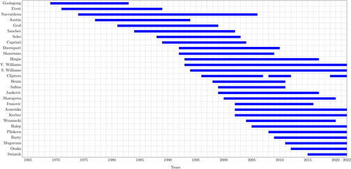
The chart shows that Navratilova and the Williams sisters have the longest career paths (although others also have careers close to 20 years). We can also see, for instance, that Clijsters retired and resumed two times during our time. There were 11 active players at the beginning of 2022 including the Williams sisters.

We use the database to support our methodology to provide a historical ranking of the selected players. Instead of building a point system from the tournament characteristics and the advancement of a player at a given tournament, we will determine the position of a player using the match results against each other. Let us say that player $P_i$ is “better” than $P_j$ if the number of her wins over $P_j$ is greater than her losses (there is no tie in tennis), and it is measured by the win/lose (W_ij/L_ij) ratio. We can construct a matrix with the names of the players in the rows and columns, where the elements are the W/L ratios. The row player is better than the column player if the corresponding ratio is larger than 1, and they are equal if the W/L ratio is 1. If the reciprocal values will measure how much “worse” $P_i$ than $P_j,$ then all of the ratios form a paired comparison matrix (PCM).

Let $P_1,P_2,\dots ,P_n$ denote the players. Our data can be described as follows: (1) $$z_{\mathit{\text{ij}}}\mathrm{ }(i,j=1,\dots ,n,i\ne j):\text{the number of matches played between}{P}_i\text{and}{P}_j\mathrm{ }(z_{\mathit{\text{ij}}}=z_{\mathit{\text{ji}}});x_{\mathit{\text{ij}}}(i>j):\text{the number of matches between}{P}_i\text{and}{P}_j,\text{where the winner was}{P}_i;y_{\mathit{\text{ij}}}=z_{\mathit{\text{ij}}}-x_{\mathit{\text{ij}}}\mathrm{ }(i>j):\text{the number of matches between}{P}_i\text{and}{P}_j,\text{where}{P}_i\text{was the loser}.$$(1)

In the incomplete $\mathit{P}=\left[p_{\mathit{\text{ij}}}\right],$ $i,j=1,\dots ,n$ pairwise comparison matrix, $p_{\mathit{\text{ij}}}$ denote the W_ij/L_ij ratio between $P_i$ and $P_j:$ (2) $$\begin{array}{l}{p}_{\mathit{\text{ij}}}=\frac{x_{\mathit{\text{ij}}}}{y_{\mathit{\text{ij}}}},\text{if}i,j=1,\dots ,n,i>j\text{and}{x}_{\mathit{\text{ij}}}\ne 0,y_{\mathit{\text{ij}}}\ne 0;\\ p_{\mathit{\text{ji}}}=y_{\mathit{\text{ij}}}/x_{\mathit{\text{ij}}}=1/p_{\mathit{\text{ij}}},\text{if}i,j=1,\dots ,n,i<j\text{and}{x}_{\mathit{\text{ij}}}\ne 0,z_{\mathit{\text{ij}}}\ne 0;\\ p_{\mathit{\text{ii}}}=1\left(i=1,\dots ,n\right);\end{array}$$(2) $p_{\mathit{\text{ij}}}$ and $p_{\mathit{\text{ji}}}$ are missing otherwise.

Similarly to Bozóki et al. (2016), we had to make data corrections to avoid the case of 0 as a denominator in W_ij/L_ij ratios: (3) $$p_{\mathit{\text{ij}}}=x_{\mathit{\text{ij}}}+2,\text{if}i>j,y_{\mathit{\text{ij}}}=0\text{and}{z}_{\mathit{\text{ij}}}\ne 0(i,j=1,\dots ,n).$$(3)

The interpretation of the $p_{\mathit{\text{ij}}}$ > 0 element is that the $i$ th player is $p_{\mathit{\text{ij}}}$ times better than the $j$ th player.

The WTA web page H2H section includes all results of the players. The W/L ratios are in Table 1. As can be seen from Table 1, the range of the $z_{\mathit{\text{ij}}}$ elements is large: therefore the range of the values of $p_{\mathit{\text{ij}}}$ is large as well. We have used the following transformation to extract the range: (4) $$t_{\mathit{\text{ij}}}=p_{\mathit{\text{ij}}}^{z_{\mathit{\text{ij}}}/K}\text{if}{z}_{\mathit{\text{ij}}}<K\text{and}{t}_{\mathit{\text{ij}}}=p_{\mathit{\text{ij}}}\mathrm{\text{otherwise}}$$(4) $$K=\underset{i,j}{\mathrm{\text{max}}}{z}_{\mathit{\text{ij}}},$$ where the transforming factor is the ratio of the number of matches played between the given two players and the maximum of the number of matches played between any two players. This can also solve the problem that the same W/L ratio based on a few matches is considered to be less reliable compared to the ratio coming from a large number of matches, so we transform the ratios based on a small sample in a way that they will be closer to one. Note that if all players have the same number of matches, transformation (4)(4) $$t_{\mathit{\text{ij}}}=p_{\mathit{\text{ij}}}^{z_{\mathit{\text{ij}}}/K}\text{if}{z}_{\mathit{\text{ij}}}<K\text{and}{t}_{\mathit{\text{ij}}}=p_{\mathit{\text{ij}}}\mathrm{\text{otherwise}}$$(4) results in $t_{\mathit{\text{ij}}}$ = $p_{\mathit{\text{ij}}}.$ If the parameter $K$ is set to a smaller value, it can be interpreted as a threshold from where we do not distinguish between the confidence of the ratios based on the number of matches. Now the initial matrix of the calculations will be matrix $\mathit{T}$ with elements $\mathrm{ }{t}_{\mathit{\text{ij}}}.$ This matrix is obviously incomplete because it is easy to find players with disjoint career intervals in Figure 1.

Table 1. W/L ratios of top WTA players.

	Goolagong	Evert	Navratilova	Austin	Graf	Sanchez	Seles	Capriati	Davenport	Mauresmo	Hingis	V. Williams	S. Williams	Clijsters	Henin	Safina	Jankovic	Sharapova	Ivanovic	Azarenka	Kerber	Wozniacki	Halep	Pliskova	Barty	Muguruza	Osaka	Swiatek
Goolagong		12/26	12/15	4/4
Evert	26/12		37/43	9/8	6/7	1/1	2/1
Navratilova	15/12	43/37		20/13	9/9	12/3	7/10	1/1	1/0
Austin	4/4	8/9	13/20		1/1
Graf		7/6	9/9	1/1		28/8	10/5	10/1	8/6	1/0	7/2	3/2	1/1	1/0
Sanchez		1/1	3/12		8/28		3/20	6/4	7/5	1/2	2/18	3/6	4/3	0/4	1/0
Seles		1/2	10/7		5/10	20/3		9/5	3/10	3/2	5/15	1/9	1/4	1/0	4/3			1/0
Capriati			1/1		1/10	4/6	5/9		3/9	4/7	4/5	0/4	7/10	3/3	2/5			1/0
Davenport			0/1		6/8	5/7	10/3	9/3		12/4	14/11	14/13	4/10	8/9	5/7	2/1	4/2	1/5	1/0		1/0	1/0
Mauresmo					0/1	2/1	2/3	7/4	4/12		7/8	3/5	2/10	7/8	6/8	4/3	6/1	3/1	6/2	0/2		0/1
Hingis					2/7	18/2	15/5	5/4	11/14	8/7		11/10	6/7	4/5	2/2	2/1	0/2	1/2	1/1	0/1		2/0
V. Williams					2/3	6/3	9/1	4/0	13/14	5/3	10/11		12/19	6/7	7/2	3/1	7/7	3/5	9/3	6/3	3/6	7/1	3/4	1/2	0/2	4/2	1/1
S. Williams					1/1	3/4	4/1	10/7	10/4	10/2	7/6	19/12		7/2	8/6	6/1	10/4	20/2	9/1	18/5	6/3	10/1	10/2	2/2	2/0	3/3	1/3
Clijsters					0/1	4/0	0/1	3/3	9/8	8/7	5/4	7/6	2/7		13/12	8/2	8/1	5/4	6/0	4/3	0/1	3/0	1/0			0/1
Henin						0/1	¾	5/2	7/5	8/6	2/2	2/7	6/8	12/13		5/1	10/0	7/3	5/0		2/0	1/0
Safina									1/2	3/4	1/2	1/3	1/6	2/8	1/5		3/4	3/4	1/3	4/2		1/0	1/0
Jankovic									2/4	1/6	2/0	7/7	4/10	1/8	0/10	4/3		1/8	3/9	4/7	2/4	5/6	1/7	1/1		2/3
Sharapova							0/1	0/1	5/1	1/3	2/1	5/3	2/20	4/5	3/7	4/3	8/1		10/4	8/7	4/5	7/4	7/2	2/0	1/2	3/1	0/1
Ivanovic									0/1	2/6	1/1	3/9	1/9	0/6	0/5	3/1	9/3	4/10		3/5	5/2	5/2	3/2	0/5		0/1
Azarenka										2/0	1/0	3/6	5/18	3/4		2/4	7/4	7/8	5/3		10/1	7/4	2/3	4/4	1/1	2/3	1/3	1/2
Kerber									0/1			6/3	3/6	1/0	0/2		4/2	5/4	2/5	1/10		8/7	6/6	7/5	2/3	3/5	4/2	0/1
Wozniacki									0/1	1/0	0/2	1/7	1/10	0/3	0/1	0/1	6/5	4/7	2/5	4/7	7/8		5/2	6/4	3/4	3/3	2/1	0/1
Halep												4/3	2/10	0/1		0/1	7/1	2/7	2/3	3/2	6/6	2/5		8/4	3/1	3/4	4/1	2/2
Pliskova												2/1	2/2				1/1	0/2	5/0	4/4	5/7	4/6	4/8		2/6	9/2	3/2
Barty												2/0	0/2					2/1		1/1	3/2	4/3	1/3	6/2		3/1	2/2	2/0
Muguruza												2/4	3/3	1/0			3/2	1/3	1/0	3/2	5/3	3/3	4/3	2/9	1/3		0/1	1/0
Osaka												1/1	3/1					1/0		3/1	2/4	1/2	1/4	2/3	2/2	1/0		1/1
Swiatek																				2/1	1/0	1/0	2/2		0/2	0/1	1/1
	Goolagong	Evert	Navratilova	Austin	Graf	Sanchez	Seles	Capriati	Davenport	Mauresmo	Hingis	V. Williams	S. Williams	Clijsters	Henin	Safina	Jankovic	Sharapova	Ivanovic	Azarenka	Kerber	Wozniacki	Halep	Pliskova	Barty	Muguruza	Osaka	Swiatek

The graph representation of Table 1 is the network in Figure 2. The vertices of the undirected graph represent the players. The edges show that the connected players played at least one match against each other. An important property of the graph representation in Figure 2 is that it is connected. According to Theorem 1, the estimated weight vector gives a unique solution.

Figure 2. Graph representation of top WTA players’ IPCM.

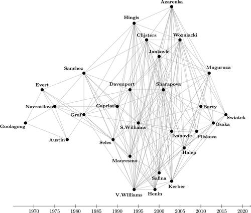
On first glance it appears that the players at the beginning and at the end of the 50-year-long period are strictly separated; however, we can find players who “connect” them, like Sharapova or the Williams sisters. Navratilova could be one of them, but she met only 8 players of the other 27: calculating career path statisticians do not distinguish between individual and double competitions, and the latter extended her professional career longer than the average.

3.2. Ranking results

The weight vector of the women players’ incomplete PCM calculated with the logarithmic least squares method gives the ranking in the first column in Table 2. The result is not surprising: Serena Williams, Graf, and Navratilova top the list, followed by Hingis, Clijsters, and Henin. The new generation is represented by Barty in the 8th place. The second column of the table demonstrates that the W/L rates prove to be a good proxy of our ranking. The Spearman rank correlation value is 0.962.

Table 2. Ranking results.

	LLSM	W/L	LLSMK=30	EV	BT
S. Williams	1	1	1	1	1
Graf	2	2	2	2	2
Navratilova	3	6	3	3	4
Hingis	4	7	4	4	7
Clijsters	5	5	5	5	6
Henin	6	4	6	6	3
V. Williams	7	8	7	7	9
Barty	8	3	8	8	10
Davenport	9	9	10	9	8
Evert	10	10	9	10	5
Seles	11	16	11	11	12
Osaka	12	14	12	13	16
Sharapova	13	11	13	12	13
Pliskova	14	12	14	14	20
Halep	15	15	15	15	19
Swiatek	16	13	16	16	17
Azarenka	17	17	17	17	18
Muguruza	18	19	18	18	21
Mauresmo	19	18	19	20	14
Kerber	20	20	20	19	22
Wozniacki	21	22	21	21	24
Safina	22	25	23	22	25
Austin	23	21	22	23	11
Ivanovic	24	24	24	24	27
Capriati	25	26	25	25	23
Jankovic	26	27	26	26	28
Sanchez	27	28	28	27	26
Goolagong	28	23	27	28	15

Since the value of the parameter $K$ is an outlier $(K=80$), a ranking was generated with an average value, $K=30,$ as can be seen in column 3. There are minor changes in the positions of the players: Evert and Davenport changed positions in the 9th and 10th places; Safina and Austin in the 22nd and 23rd positions; Sanchez and Goolagong changed the last two positions. The Spearman rank correlation value is 0.998. The situation was similar to other transformation factors. The fourth column of the table contains the ranking calculated with the eigenvector method. Two rank reversals can be found: Osaka and Sharapova, and Mauresmo and Kerber. The Spearman rank correlation is 0.999.

We also applied the well-known, probability-based Bradley-Terry model (Bradley & Terry, 1952) to our data to create a ranking, and compare this approach to ours. This method assumes that there are latent random variables with logistic distribution behind the performance of the players. In the traditional model we are estimating the expected values of these random variables and based on those we can rank the objects (the larger the better). Usually, the maximum likelihood estimation method is used to determine the parameters (expected values), for which there exists a unique solution if and only if the directed graph of the comparisons is strongly connected (Ford, 1957). This assumption is more stringent than the uniqueness of the PCM-based method. It basically means that even that graph should be connected, for which we delete those edges from the graph of Figure 2 where only one of the players has won all the matches. This means 40 of the 192 edges in our data, however, this graph is still connected. We calculated the results of the Bradley-Terry model to compare our method to one of the most commonly used probability-based ranking methods as well. Column 5 of the table contains the ranking calculated with the maximum likelihood method of the Bradley-Terry model. As one can see, the BT-model provides a similar ranking, and the Spearman rank correlation is 0.860. The main difference is that the ranks of the earlier players (Goolagong, Evert, Austin, and Henin) are significantly better.

Our calculations with the WTA players are in line with the top ATP players in Bozóki et al. (2016). Both data systems are robust in that respect that the rankings which have been calculated from the incomplete PCMs are not sensitive to reasonable corrections, and the choice of the estimation method does not make a significant impact on the results. The rankings are similar to other orders determined by commonly used ranking models, like the Bradley-Terry method. Empirical evidence suggests that our methodology can be recommended for the given ranking exercise.

The next step of our calculations was to analyse the submatrices of the initial matrix. What happens if elements (players) were dropped or involved? How do subrankings behave? PCM1 column of Table 3 shows a ranking without the first nine players in the overall ranking. Seles, Sharapova, and Evert have the first three positions; Osaka, Kerber, and Muguruza lost several positions; the last positions did not change significantly. PCM2 is a ranking without the last nine players of the overall ranking. Serena Williams and Graf saved the first two positions, but the ranking behind them is very different from the original one. The position of Seles is very interesting: in PCM1, she is first, but in PCM2, she is last! The explanation of the changes is simple and plausible. Both the number of matches and the composition of matches changed. Some players benefitted from the modified structure (those players were missing with whom they had the poorest W/L ratios), and others became victims of the changes (their best W/L ratios disappeared). Some indirect impacts have also vanished. The most prominent example of this phenomenon is Monica Seles. The rankings are not independent of the incoming and outgoing elements—as was expected.

Table 3. Ranking results from various submatrices of matrix $\mathrm{ }\mathit{T}.$

	PCM1	PCM2	PCM3	PCM4	PCM5
S. Williams	–	1	–	1	–
Graf	–	2	–	–	1
Navratilova	–	8	1	–	2
Hingis	–	9	–	6	3
Clijsters	–	10	–	2	4
Henin	–	12	–	3	5
V. Williams	–	5	–	4	–
Barty	–	3	–	–	10
Davenport	–	7	–	5	6
Evert	3	18	2	–	–
Seles	1	19	–	–	–
Osaka	12	6	–	–	15
Sharapova	2	15	–	7	8
Pliskova	6	4	–	–	13
Halep	7	11	–	–	14
Swiatek	8	13	–	–	–
Azarenka	5	16	–	–	–
Muguruza	14	14	–	–	16
Mauresmo	4	17	–	8	11
Kerber	15	–	–	–	–
Wozniacki	11	–	–	11	12
Safina	9	–	–	9	–
Austin	18	–	3	–	7
Ivanovic	10	–	–	10	18
Capriati	13	–	–	–	17
Jankovic	17	–	–	12	–
Sanchez	16	–	–	–	19
Goolagong	19	–	4	–	9

PCM3 is the ranking of the four most influential stars of the seventies. They follow each other under the overall ranking: it looks like their results inside of PCM3 follow the pattern outside of the block. Since everybody played against everybody here, a simple preference order can be calculated based on the winner-loser relationship as a binary relation. The order is Navratilova $\succ$ Evert $\succ$ Austin $\sim$ Goolagong. PCM4 is a ranking of 12 players from the next era. From the first six places, Hingis is the only one, who lost position, and Wozniacki is the other one, who lost position at the end of the ranking. PCM4 gives evidence that it is possible to select a relatively large number of players with their most active career in the same time period, so that their results practically determine their positions with minor changes compared to the overall ranking. PCM3 and PCM4 are complete submatrices of matrix $\mathrm{ }\mathit{T},$ therefore the usual $\mathit{\text{CR}}$ inconsistency indices can be calculated, too. The $\mathit{\text{CR}}$ values are below 0.02 supporting our hypothesis about the robustness of the data. Furthermore, PCM4 includes 20.50% of all matches in the matrix $\mathrm{ }\mathit{T}.$

Finally, in PCM5 there is a ranking of 19 players selected randomly from our pool of women players. The Williams sisters, Evert, Seles, Kerber, Azarenka, Safina, Jankovic, and Swiatek were not included. The first five players follow each other in the same order as they did in the overall ranking. The reason is likely the fact that their performance against Evert and the Williams sisters follows the same pattern not influencing the ranking based on their match results against each other. Due to the elimination of their results against the leaving players, Sharapova and Austin are in a better position. We have had the same experience with other random sets of players.

There are two key conclusions from these calculations. Changes in the set of players changed the rankings—as we expected. However, these changes did not blow over the original rankings entirely, the new positions could be explained with the new patterns of the modified PCM.

We also examined the rankings, when we added additional elements (tennis players) to the set of players one by one. The first subset that we analysed includes the players who were active at the beginning of 2022 (11 players). Then we stepped backward in time and included the next player, who finished her professional career the latest (in case of a tie between two players, we chose the one who started her career later). We included the elements one by one until we get the whole ranking of all 28 players. In this way, we generated 18 different rankings, which can be seen in Figure 3, as well as the changes caused by the entry of a given player (the entering players are shown at the bottom of the chart). It is important to note that there are exactly as many rank reversals due to the inclusion of a given player, as many lines cross each other between the inclusion and the former player’s involvement.

Figure 3. The differences in the rankings of women tennis players when they enter the ranking one by one.

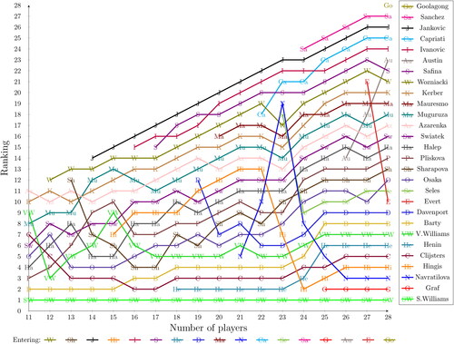
We can see that the ranking is robust, the inclusion of a player usually does not affect the results too much, and only one or two rank reversals occur. In the rare cases when a player’s rank is changed by a significant number it is since she barely played with the other players who are in the ranking so far (for instance Austin), and her comparison to the newly involved element (Evert, and then Goolagong) is more reliable. This can be seen, when the ranking of Navratilova undergoes a lot of change in the first few steps as she only played a single match with the so far included players. Of course, a player may also win (or lose) many times against a currently entered element (for instance Hingis against Seles or Sanchez and Venus Williams against Ivanovic). It is worth mentioning that the entry of a player usually has a larger impact on the players with whom she has played a lot. The beginning and the end of the ranking both seem to be robust. We can see more rank reversals in the middle, as we involve more and more elements. However, it still looks like there are clusters here, and the ranking of the players only changes within those groups.

3.3. Graph representations

Using graph representations gave us the possibility to have a deeper insight into the properties of incomplete pairwise comparison matrices. The representing graph of the women players can be seen in Figure 1, while its connectivity indicators are described in Table 4.

Table 4. Properties of the representing graph for WTA players.

	WTA	WTAmod
Number of vertices (players)	28	23
Number of edges (players compared)	192	170
Minimal vertex degree	3	9
Maximal vertex degree	22	22
Diameter	4	2
Average shortest path	1.66	1.33
Edge connectivity	3	9
Vertex connectivity	3	8

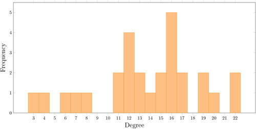
We can find one player (Goolagong), who had competitions with only three other players, as it is indicated by the minimal vertex degree. On the contrary, the Williams sisters had matches with 22 other players. The maximal vertex degree belongs to them. Erasing either any 2 edges or vertices we can get a connected graph. The longest shortest path (diameter) is 4, and it can be determined between players far from each other in time: Goolagong and Osaka/Muguruza/Barty/Swiatek respectively or between Evert and Swiatek.

Figure 4 illustrates the degree of vertices. That distribution is used in network theory (Albert et al., 2000) for analysing various types of systems. In our case, the average shortest path has a small value, and the degrees are distributed relatively orderly around the average. The clustering value is 0.79 (that means certain groups of players have results from the same group). These properties indicate that our network is a small-world type one (Watts & Strogatz, 1998).

Figure 4. Distribution of the degree of vertices.

Another feature of the representing graph for WTA players is that by erasing the Williams sisters, represented by the vertices with maximal vertex degree, the connectivity properties practically do not change. However, erasing the critical triads of Evert, Navratilova, and Graf, or Evert, Navratilova, and Austin, the connectivity of the graph will be lost. On the other hand, erasing four players of the earliest period (Goolagong, Evert, Navratilova, Austin) and the most recent world number one (Swiatek), the remaining graph will have much stronger connectivity indicators, as can be seen in the second column of Table 4 (WTA_mod). Rankings generated from these reduced graphs (submatrices) almost follow the positions in the overall ranking, suggesting that these strong relations can specify them.

It is another fact that the modified, strongly connected graph is the union of two star graphs, complemented with a few edges. The centres are the Williams sisters –meaning they played directly with all other players. Similar representing graphs can be obtained by applying the popular best-worst method (Rezaei, 2015). That structure can also be responsible for the robustness of our ranking results.

Another line of our research referred to the ordinally nontransitive triads. There are many sports competitions where W/L > 1 for A and B, and the same is true for B and C: A is better than B, and B is better than C. We can expect that A will be better than C; however, from the results, we get W/L < 1. In preference ordering that triad is called contradictory (Kwiesielewicz & van Uden, 2004). A suitable example of an ordinally nontransitive triad is Henin, Davenport, and Venus Williams in our database. We chose the positive reciprocal multiplicative PCM approach for ranking tennis players because the estimation methods are functional in the case of ordinal or cardinal nontransitivity. However, in the course of discussing the ranking results, it is important to know more about the ordinally nontransitive triads of the PCM, since their presence signals a kind of contradiction. Representing graphs are directed in the analysis of ordinal nontransitivity: an edge leads from one player to the next if the latter player lost more matches.

Kendall and Babington Smith (1940) gave the distribution of ordinally nontransitive triads in the case of a low number of elements ($n\le 7$) and proposed a significance test. Alway (1962) extended the distribution for $8\le n\le 10;$ others analysed cases with larger numbers of elements. Moran (1947) proved that the distribution of the nontransitive triads goes to the normal distribution if the number of elements goes to infinity, but the convergence is slow. Knezek et al. (1998) investigated the chi-square distribution used by Kendall and Babington Smith (1940) earlier, and they found it satisfactory for more than 15 elements. Jensen and Hicks (1993) proposed a consistency coefficient and a nonparametric test for ordinal PCMs, while Iida (2009) discussed the nontransitivity tests for decision-making problems by applying them to binary PCMs without ties. It is crucial to note that all of the above-mentioned tests worked for complete PCMs without ties. In the case of ties, Kułakowski (2018) determined the maximal number of contradictory triads for any number of elements and proposed an index related to that number (without a statistical test). He extended the definition of contradictory triads to those cases when there are only one or two equalities between the elements of the triads. That kind of inconsistency analysis could not be interpreted properly in our case; we are looking for strictly inconsistent triads. That is why we did not follow the approaches of Iida or Kułakowski, and decided to hark back to the case without ties and to use the known tests.

The modified databases contain W/L set ratios for each pair. In the case of having ties even for the set ratios, the original LLSM ranking was the reference to make a precedence relation. The nontransitivity tests need complete matrices. If two players have not played with each other for any reason (no edge was found between the two vertices), then we used the same reference ranking to determine a “winner.” A complete directed graph was created this way. Table 5 includes information about the original incomplete PCM in the first, and about its completed and tie-corrected version in the second column.

Table 5. Basic data for nontransitivity analysis.

	WTA	WTAcomplete
Density	192/378	378/378
Number of ties	20	0
Number of ordinally nontransitive triads	83	315
Possible maximal number of ordinally nontransitive triads	910	910

Regarding the case before correction, we can see that the PCM has a density of around 50% (half of the elements are known), and the ratio of ties is about 10%. We have got the number of nontransitive triads from the incomplete matrices here, therefore it is not comparable with the possible maximal number of nontransitive triads obtained from the complete matrix. The second column of Table 5 informs us about the case after eliminating ties and completing the matrix. The chi-squared test value is ∼202, the corresponding $p$-value is practically 0: the number of ordinally nontransitive triads is not significant in our database.

4. Conclusion

Our results provide empirical evidence that the method of incomplete pairwise comparison matrices is appropriate for producing well-understood rankings. Our study was based on the match results of players against each other. Calculations with the whole databases and their subsets clarified that WTA data were robust enough to state that although the rankings have been changed, the differences can be explained via the analysis of the data matrices, and they are logically consistent. Our historical rankings alone may be of interest to tennis experts, but they are also relevant from a decision theory perspective.

One of the novelties of our approach was the analysis of representing graphs. We aimed to contribute to a deeper description of the properties of incomplete pairwise comparison matrices. Graph representations can open new avenues in this regard. We consider further research on ordinally nontransitive triads to be particularly important.

Our work is based on Head-to-Head statistics of the players without taking some considerations into account, which seems to limit the validity of our rankings. They are listed and commented on here with the aim of either explaining why we chose an overall and unified approach or opening new tracks with fine-tuning of the data.

Tennis fans and experts can say that: “It is not fair to give the same weight to the matches of any player from the very early and very late periods of their professional career.” Having details about the professional career of each player it is possible to introduce correction factors. But there are at least two reasons to drop the idea. It would not be easy to determine those early and late stages, and even if we can do it, the value of the correction parameter would include a strong subjective factor in the analysis. On the other hand, we can easily find players with exceptionally good early results (e.g., Austin, Seles, Osaka), and some players retired without a declining period (e.g., Henin). That kind of time-dependent adjustment of data would bring a very controversial factor to the ranking results.

„Different surfaces need another sort of treatment.” The weighting of surfaces would introduce a subjective factor, again. Revaluation of individual results would lead to endless debates. Yes, a viable solution would be to make separate rankings for different surfaces: who is the top player on clay court, and who is the most successful on grass? Data are available, but we did not undertake that job, because it would not give extra methodological benefits.

„Match ratios can be used, but set ratios would reflect better to power differentiation.” Data are available to calculate W/L ratios from sets. We have made some calculations in the case of both men and women players. Rankings were not significantly different from the original ones, so we dropped that artificial approach.

„Ranking is restricted to the No. 1 WTA players—their performance against other players might change that ranking.” For instance, selecting the top 20 players from every year between 1973 and 2022 is possible, as data are available. We have not done the job of ranking them (or more players). It is worth mentioning that historical rankings of different player populations show very strong similarity (as is referred to in the introductory section of this article). Another remark is that top tennis is surprisingly endogenous, the best players meet each other frequently. Even in our small sample, we can see that the ratio of “number of matches in our database/number of matches in the entire career” is the smallest for Swiatek (∼6%), and the largest for Serena Williams (∼25%).

Correction Statement

This article has been corrected with minor changes. These changes do not impact the academic content of the article.

Acknowledgements

The authors thank the valuable comments and suggestions of the anonymous Reviewers. The comments of László Csató and András London are greatly acknowledged. This research has been supported in part by the TKP2021-NKTA-01 NRDIO grant.

Disclosure statement

No potential conflict of interest was reported by the authors.

Notes

1 https://www.atptour.com/, https://www.wtatennis.com

2 https://www.atptour.com/en/rankings/singles, https://www.wtatennis.com/rankings/singles

3 https://en.wikipedia.org/wiki/List_of_WTA_number_1_ranked_tennis_players

References

- Ágoston, K. C., & Csató, L. (2022). Inconsistency thresholds for incomplete pairwise comparison matrices. Omega, 108, 102576. https://doi.org/10.1016/j.omega.2021.102576
- Albert, R., Jeong, H., & Barabasi, A. (2000). Error and attack tolerance of complex networks. Nature, 406(6794), 378–382. https://doi.org/10.1038/35019019
- Alway, G. G. (1962). The distribution of the number of circular triads in paired comparisons. Biometrika, 49(1–2), 265–269. https://doi.org/10.1093/biomet/49.1-2.265
- Anholcer, M., & Fülöp, J. (2019). Deriving priorities from inconsistent PCM using network algorithms. Annals of Operations Research, 274(1–2), 57–74. https://doi.org/10.1007/s10479-018-2888-x
- Baker, R. D., & McHale, I. G. (2014). A dynamic paired comparisons model: Who is the greatest tennis player? European Journal of Operational Research, 236(2), 677–684. https://doi.org/10.1016/j.ejor.2013.12.028
- Baker, R. D., & McHale, I. G. (2017). An empirical Bayes model for time-varying paired comparisons ratings: Who is the greatest women’s tennis player? European Journal of Operational Research, 258(1), 328–333. https://doi.org/10.1016/j.ejor.2016.08.043
- Bozóki, S., Fülöp, J., & Rónyai, L. (2009). Incomplete pairwise comparison matrices in multi-attribute decision making. In Proceedings of the 2009 IEEE IEEM [Paper presentation]. 2256–2260. https://doi.org/10.1109/IEEM.2009.5373064
- Bozóki, S., Csató, L., & Temesi, J. (2016). An application of incomplete pairwise comparison matrices for ranking top tennis players. European Journal of Operational Research, 248(1), 211–218. https://doi.org/10.1016/j.ejor.2015.06.069
- Bozóki, S., Fülöp, J., & Rónyai, L. (2010). On optimal completion of incomplete pairwise comparison matrices. Mathematical and Computer Modelling, 52(1–2), 318–333. https://doi.org/10.1016/j.mcm.2010.02.047
- Bozóki, S., & Tsyganok, V. (2019). The (logarithmic) least squares optimality of the arithmetic (geometric) mean of weight vectors calculated from all spanning trees for incomplete additive (multiplicative) pairwise comparison matrices. International Journal of General Systems, 48(4), 362–381. https://doi.org/10.1080/03081079.2019.1585432
- Bradley, R. A., & Terry, M. E. (1952). Rank analysis of incomplete block designs. Biometrika, 39(3/4), 324–345. https://doi.org/10.2307/2334029
- Brin, S., & Page, L. (1998). The anatomy of a large-scale hypertextual Web search engine. Computer Networks and ISDN Systems, 30(1-7), 107–117. https://doi.org/10.1016/S0169-7552(98)00110-X
- Brunelli, M. (2014). Introduction to the analytic hierarchy process. Springer. https://doi.org/10.1007/978-3-319-12502-2
- Brunelli, M. (2018). A survey of inconsistency indices for pairwise comparisons. International Journal of General Systems, 47(8), 751–771. https://doi.org/10.1080/03081079.2018.1523156
- Brunelli, M., & Fedrizzi, M. (2015). Axiomatic properties of inconsistency indices for pairwise comparisons. Journal of the Operational Research Society, 66(1), 1–15. https://doi.org/10.1057/jors.2013.135
- Crawford, G., & Williams, C. (1985). A note on the analysis of subjective judgment matrices. Journal of Mathematical Psychology, 29(4), 387–405. https://doi.org/10.1016/0022-2496(85)90002-1
- Csató, L. (2021). Tournament design. How operations research can improve sports rules? Palgrave Pivots in Sports Economics. https://doi.org/10.1007/978-3-030-59844-0
- Dahl, G. (2012). A matrix-based ranking method with application to tennis. Linear Algebra and Its Applications, 437(1), 26–36. https://doi.org/10.1016/j.laa.2012.02.002
- Dingle, N., Knottenbelt, W., & Spanias, D. (2012). On the (page) ranking of professional tennis players. In M. Tribastone & S. Gilmore (Ed.), Computer performance engineering (pp. 237–247). Springer. https://doi.org/10.1007/978-3-642-36781-6_17
- Elo, A. E. (1978). The rating of chessplayers, past and present. Arco Pub. https://www.gwern.net/docs/statistics/comparison/1978-elo-theratingofchessplayerspastandpresent.pdf
- Ford, L. R. Jr. (1957). Solution of a ranking problem from binary comparisons. The American Mathematical Monthly, 64(8P2), 28–33. https://doi.org/10.2307/2308513
- Gass, S. (1998). Tournaments, transitivity and pairwise comparison matrices. Journal of the Operational Research Society, 49(6), 616–624. https://doi.org/10.1057/palgrave.jors.2600572
- Gu, W., & Saaty, T. L. (2019). Predicting the outcome of a tennis tournament: Based on both data and judgments. Journal of Systems Science and Systems Engineering, 28(3), 317–343. https://doi.org/10.1007/s11518-018-5395-3
- Iida, Y. (2009). The number of circular triads in a pairwise comparison matrix and a consistency test in the AHP. Journal of the Operations Research Society of Japan, 52(2), 174–185. https://doi.org/10.15807/jorsj.52.174
- Jensen, R. E., & Hicks, T. E. (1993). Ordinal data AHP analysis: A proposed coefficient of consistency and a nonparametric test. Mathematical and Computer Modelling, 17(4-5), 135–150. https://doi.org/10.1016/0895-7177(93)90182-X
- Keener, J. P. (1993). The Perron-Frobenius theorem and the ranking of football teams. SIAM Review, 35(1), 80–93. https://doi.org/10.1137/1035004
- Kendall, M. G. (1955). Further contributions to the theory of paired comparisons. Biometrics, 11(1), 43–62. https://doi.org/10.2307/3001479
- Kendall, M. G., & Babington Smith, B. (1940). On the method of pairwise comparisons. Biometrika, 31(3-4), 324–345. https://doi.org/10.2307/2332613
- Knezek, G., Wallace, S., & Dunn-Rankin, P. (1998). Accuracy of Kendall’s chi-square approximation to circular triad distributions. Psychometrika, 63(1), 23–34. https://doi.org/10.1007/BF02295434
- Kovalchik, S. A. (2016). Searching for the GOAT of tennis win prediction. Journal of Quantitative Analysis in Sports, 12(3), 127–138. https://doi.org/10.1515/jqas-2015-0059
- Kułakowski, K. (2018). Inconsistency in the ordinal pairwise comparisons method with and without ties. European Journal of Operational Research, 270(1), 314–327. https://doi.org/10.1016/j.ejor.2018.03.024
- Kułakowski, K., Mazurek, J., & Strada, M. (2021). On the similarity between ranking vectors in the pairwise comparison method. Journal of the Operational Research Society, 73(9), 2080–2089. https://doi.org/10.1080/01605682.2021.1947754
- Kwiesielewicz, M., & van Uden, E. (2004). Inconsistent judgments in pairwise comparison method in the AHP. Computers & Operations Research, 31(5), 713–719. https://doi.org/10.1016/S0305-0548(03)00022-4
- Langville, A. N., & Meyer, C. D. (2006). Google’s PageRank and beyond: The science of search engine rankings. Princeton University Press. https://www.jstor.org/stable/j.ctt7t8z9
- Langville, A. N., & Meyer, C. D. (2012). Who’s #1? The science of rating and ranking. Princeton University Press. https://www.jstor.org/stable/j.ctt7rwdt
- Lisi, F., & Zanella, G. (2017). Tennis betting: Can statistics beat bookmakers? Electronic Journal of Applied Statistical Analysis, 10(3), 790–808. http://siba-ese.unisalento.it/index.php/ejasa/article/view/16516
- Moran, P. A. P. (1947). On the method of paired comparisons. Biometrika, 34(Pt 3–4), 363–365. https://pubmed.ncbi.nlm.nih.gov/18918706/
- Orbán-Mihálykó, É., Mihálykó, C., & Koltay, L. (2019). A generalization of the Thurstone method for multiple choice and incomplete paired comparisons. Central European Journal of Operations Research, 27(1), 133–159. https://doi.org/10.1007/s10100-017-0495-6
- Ramón, N., Ruiz, J. L., & Sirvent, I. (2012). Common sets of weights as summaries of DEA profiles of weights: With an application to the ranking of professional tennis players. Expert Systems with Applications, 39(5), 4882–4889. https://doi.org/10.1016/j.eswa.2011.10.004
- Rezaei, J. (2015). Best-worst multi-criteria decision-making method. Omega, 53, 49–57. https://doi.org/10.1016/j.omega.2014.11.009
- Saaty, T. L. (1977). A scaling method for priorities in hierarchical structures. Journal of Mathematical Psychology, 15(3), 234–281. https://doi.org/10.1016/0022-2496(77)90033-5
- Saaty, T. L. (1987). Rank according to Perron: A new insight. Mathematics Magazine, 60(4), 211–213. https://doi.org/10.2307/2689340
- Shiraishi, S., Obata, T., & Daigo, M. (1998). Properties of a positive reciprocal matrix and their application to. Journal of the Operations Research Society of Japan, 41(3), 404–414. https://doi.org/10.15807/jorsj.41.404
- Szádoczki, Zs., Bozóki, S., & Tekile, H. A. (2022). Filling in pattern designs for incomplete pairwise comparison matrices: (Quasi-)regular graphs with minimal diameter. Omega, 107(C), 102557. https://doi.org/10.1016/j.omega.2021.102557
- Thurstone, L. L. (1927). A law of comparative judgment. Psychological Review, 34(4), 273–286. https://doi.org/10.1037/h0070288
- Vaughan-Williams, L., Liu, C., & Gerrard, H. (2019). How well do Elo-based ratings predict professional tennis matches? NBS Discussion Papers in Economics, 2019/03. Nottingham Business School, Nottingham Trent University. https://doi.org/10.1515/jqas-2019-0110
- Wang, H., Peng, Y., & Kou, G. (2021). A two-stage ranking method to minimize ordinal violation for pairwise comparisons. Applied Soft Computing, 106, 107287. https://doi.org/10.1016/j.asoc.2021.107287
- Watts, D. J., & Strogatz, S. H. (1998). Collective dynamics of ’small-world’ networks. Nature, 393(6684), 440–442. https://doi.org/10.1038/30918
- Wei, T. H. (1952). The algebraic foundations of ranking theory [PhD thesis]. Cambridge University. https://www.repository.cam.ac.uk/handle/1810/250988