Socially responsible multiobjective optimal portfolios

Abstract

This article extends the socially responsible multiobjective problem to (i) estimating optimal portfolios via reward/risk maximization, (ii) including dependence structure between asset returns using vine copulas, and (iii) incorporating enhanced indexation utilizing cumulative zero-order stochastic dominance (CZϵSD). Applying the multiobjective optimal portfolio (MOOP) approach to a sample of EuroStoxx 50 constituents, the results show that the MOOPs provide investors with the flexibility to incorporate different objectives while investing in optimal portfolios. Including social responsibility results in lower portfolio return and economic performance, but at the same time portfolio risk, expected shortfall of portfolio returns below the benchmark, and turnover are reduced. The copula-based predictive models lead to MOOPs with higher returns and reward/risk ratios. Moreover, optimizing environmental scores leads to less risky MOOPs, while optimizing social scores results in higher average return and better risk-adjusted performance.

Keywords:

• Finance
• multiobjective portfolio
• reward/risk maximization
• vine copula
• conditional value at risk
• zero-order stochastic dominance

1. Introduction

Asset managers and portfolio owners increasingly consider corporate social responsibility in their investment decisions. A common approach to measure social responsibility for investments is to use ESG scores (Gasser et al., 2017; Hirschberger et al., 2013; Utz et al., 2014, 2015; Lindquist et al., 2022). These scores consist of environmental, social, and governance components and are provided by several rating agencies. One apparent question is then how to incorporate ESG information when constructing socially responsible optimal portfolios. Previous literature has suggested several techniques for obtaining socially responsible multiobjective portfolios (MOP). For instance, considering both financial and ethical aspects in the expected utility function, Ballestero et al. (2012) formulate a bi-criteria portfolio problem for socially responsible and green investment and show that the classical mean-variance framework provides higher returns and lower risk compared to the highly green investments. Hirschberger et al. (2013) suggest a quadratic programming approach to extend Markowitz’s mean-variance model to a tri-criteria portfolio problem and provide results indicating better risk and return performance for socially responsible portfolios compared to a naive equally weighted strategy. Applying inverse tri-criterion optimization, Utz et al. (2014) conclude that there is no difference between conventional and socially responsible mutual funds in terms of asset allocation. Xidonas et al. (2012), Aouni et al. (2018), and Masmoudi and Abdelaziz (2018) provide a review of the different programming approaches for solving the socially responsible MOP problem.

The MOP problem can be used to estimate a Pareto frontier, including portfolios that are efficient in regard to several portfolio attributes. Then, given the investor’s preferences, one can choose the most suitable portfolio from the Pareto set. However, the investor might be interested in investing in efficient portfolios with the highest reward/risk ratio (we refer to these portfolios as optimal). Therefore, this article aims to generalize the reward/risk maximization to incorporate multiple portfolio objectives including ESG scores. Our multiobjective optimal portfolio (MOOP) approach turns out to be a special case of socially responsible MOP optimization where both the portfolio return and ESG scores are incorporated as reward measures in a reward/risk maximization. We combine fractional programming techniques developed by Charnes and Cooper (1962) and Stoyanov et al. (2007) with the weighted-sum approach used in the MOP models (Steuer, 1986; Martel et al., 1988; Ballestero & Romero, 1996; Bilbao et al., 2006; Bilbao-Terol et al., 2016; Xidonas et al., 2017; Masmoudi & Abdelaziz, 2018; Henriques & Neves, 2019).

We suggest a novel approach to construct socially responsible MOOPs with several portfolio criteria including expected return, corporate social responsibility measured by ESG scores, conditional Value-at-Risk (CVaR), turnover, and cumulative zero-order stochastic dominance (CZϵSD). Furthermore, Rvine copula models are applied to estimate step-ahead multivariate distribution for asset returns.

This article contributes to the existing literature in several important aspects. First, it develops a MOOP framework that can be used to estimate optimal (maximum reward/risk) portfolios while allowing investors to have preferences on several portfolio criteria. To the best of our knowledge, this is the first study to combine a fractional programming technique with the MOP. In particular, our MOOP approach allows us to obtain optimal (maximum reward/risk) points directly from a multicriteria Pareto frontier set. An interesting application of the MOOP portfolio approach is social responsibility via ESG scores, where a socially responsible reward/risk maximizer is searching for an optimal strategy given her preferences for several portfolio attributes. In this case, our socially responsible MOOP approach extends the literature on sustainable investing and socially responsible MOP (Ballestero et al., 2012; Utz et al., 2014, 2015; Gasser et al., 2017; Pedersen et al., 2021; Steuer & Utz, 2023). Second, this article incorporates an enhanced indexation approach in a MOOP setting. Several approaches are suggested for enhanced indexation through second-order stochastic dominance (see e.g. Roman et al., 2013; Sharma et al., 2017; Goel & Sharma, 2021). We follow one of the recent approaches suggested by Bruni et al. (2017) and incorporate the CZϵSD, which corresponds to the expected shortfall of portfolio returns below the market returns. Third, it develops Rvine-copula-based MOOP. This makes this study one of the first to incorporate copulas in socially responsible investing.

Using a sample of constituents of the EuroStoxx 50 index, the out-of-sample performance of the suggested socially responsible MOOP strategies is examined. In particular, the main focus is on evaluating how corporate social responsibility affects the performance of MOOPs. Incorporating the ESG scores results in socially responsible MOOPs with lower volatility, CVaR, CZϵSD, and turnover. Moreover, optimizing environmental scores leads to MOOPs with lower risk, while optimizing social scores results in higher average return and risk-adjusted performance. The results of our empirical evaluation demonstrate a high flexibility of the suggested MOOP approach in terms of the portfolio criteria.

The remainder of this article is structured as follows: Section 2 presents the portfolio objectives and MOOP formulation. Section 3 presents the steps involved in constructing the copula-based MOOPs. We provide our empirical analysis in Section 5. Finally, concluding remarks are presented in Section 6.

2. Portfolio parametrization

In this section, we elaborate and introduce our suggested MOP and MOOP approaches. In general, the MOOP model is different from the MOP approach because it includes a reward/risk maximization portfolio problem. While in the MOP model, we use a weighted-sum approach to estimate Pareto efficient portfolios, in the MOOP problem, we are interested in finding those Pareto frontier portfolios with maximum reward/risk ratio (see Section 5.1 for an empirical example). In Section 2.3, we describe the benchmark portfolios used in the empirical analysis.

2.1. MOP

In a MOP problem, there are several objective functions to be maximized (or minimized). To solve such a portfolio problem, different approaches have emerged in the MOP literature including the weighted-sum, ϵ-constraint, goal, and compromise programming (see Masmoudi & Abdelaziz, 2018, for a comparison of different methods). Let ${\Lambda }_k({\widehat{\mathbf{w}}}_t)$ be a reward function and ${\psi }_q({\widehat{\mathbf{w}}}_t)$ be a risk measure. In the weighted-sum approach, the weights assigned to the objective functions, i.e. ${\lambda }_{{\Lambda }_k},{\lambda }_{{\psi }_q}\in [0,1],$ correspond to the investor’s preferences. Furthermore, there are several approaches to normalize the objective functions (see e.g. Cao et al., 2017; Xidonas et al., 2017). One approach is the linear normalization (scaling) using the so-called utopia and nadir points. Let ${\overline{\Lambda }}_k$ and ${\overline{\psi }}_q$ denote the utopia solutions, and ${\underset{¯}{\Lambda }}_k$ and ${\underset{¯}{\psi }}_q$ are the nadir points. Using the weighted-sum approach, a MOP with K + Q criteria is defined as: (1) $$\begin{array}{cccccc}\hfill & \underset{{\widehat{\mathbf{w}}}_t}{\text{minimize}}\hfill & \hfill & \sum _{q=1}^Q{\lambda }_{{\psi }_q}\left[\frac{{\psi }_q({\widehat{\mathbf{w}}}_t)}{{\underset{¯}{\psi }}_q-{\overline{\psi }}_q}\right]-\hfill & \hfill & \hfill \\ \hfill & \hfill & \hfill & \sum _{k=1}^K{\lambda }_{{\Lambda }_k}\left[\frac{{\Lambda }_k({\widehat{\mathbf{w}}}_t)}{{\overline{\Lambda }}_k-{\underset{¯}{\Lambda }}_k}\right]\hfill & \hfill & \hfill \\ \hfill & \text{subject to}\hfill & \hfill & {\widehat{\mathbf{w}}}_t^{⊺}\mathbf{1}=1\hfill & \hfill & \hfill \\ \hfill & \hfill & \hfill & {\widehat{w}}_{\mathit{\text{jt}}}\ge 0,\forall j\in \{1,2,..,d\}\hfill & \hfill & \hfill \end{array}$$(1) where ${\sum }_{q=1}^Q{\lambda }_{{\psi }_q}+{\sum }_{k=1}^K{\lambda }_{{\Lambda }_k}=1,$ and the utopia solutions are obtained from separate (individual) optimizations s.t. $\forall k\in \{1,2,\dots ,K\}:{\overline{\Lambda }}_k=\underset{{\widehat{\mathbf{w}}}_t}{\mathrm{\text{max}}} {\Lambda }_k({\widehat{\mathbf{w}}}_{{\Lambda }_k})$ and $\forall q\in \{1,2,\dots ,Q\}:{\overline{\psi }}_q=\underset{{\widehat{\mathbf{w}}}_t}{\mathrm{\text{min}}} {\psi }_q({\widehat{\mathbf{w}}}_{{\psi }_q}).$ For nadir solutions, we have $\forall k\in \{1,2,\dots ,K\}:{\underset{¯}{\Lambda }}_k=\mathrm{\text{min}}({\Lambda }_k({\widehat{\mathbf{w}}}_{{\Lambda }_1}),\dots ,{\Lambda }_k({\widehat{\mathbf{w}}}_{{\Lambda }_K}),{\Lambda }_k({\widehat{\mathbf{w}}}_{{\psi }_1}),\dots ,{\Lambda }_k({\widehat{\mathbf{w}}}_{{\psi }_Q}))$ and $\forall q\in \{1,2,\dots ,Q\}:{\underset{¯}{\psi }}_q=\mathrm{\text{max}}({\psi }_q({\widehat{\mathbf{w}}}_{{\Lambda }_1}),\dots ,{\psi }_q({\widehat{\mathbf{w}}}_{{\Lambda }_K}),{\psi }_q({\widehat{\mathbf{w}}}_{{\psi }_1}),\dots ,{\psi }_q({\widehat{\mathbf{w}}}_{{\psi }_Q})).$¹

To construct socially responsible MOP, we incorporate the five objective functions, including portfolios’ expected return, CVaR, CZϵSD, ESG score, and turnover, described in Section S2 in the online appendix. The portfolio turnover has an optimal solution of zero, i.e. ${\overline{\psi }}_{\vartheta }=0.$ Using the suggested linear transformations of portfolios’ CVaR, CZϵSD, and turnover, i.e. defining auxiliary variables $\mathbf{y},\mathbf{g},\mathit{\upsilon },$ we obtain the socially responsible MOP problem as: (2) $$\begin{array}{cccccc}\hfill & \underset{\widehat{{\mathbf{w}}_t},\mathbf{y},\mathbf{g},\mathit{\upsilon }}{\text{minimize}}\hfill & \hfill & {\lambda }_{{\psi }_{\zeta }}\left[\frac{l+{[M(1-\alpha )]}^{-1}\sum _{m=1}^M{\upsilon }_m}{{\underset{¯}{\psi }}_{\zeta }-{\overline{\psi }}_{\zeta }}\right]+{\lambda }_{{\psi }_{\delta }}\left[\frac{\sum _{m=1}^M{y}_m}{{\underset{¯}{\psi }}_{\delta }-{\overline{\psi }}_{\delta }}\right]+\hfill & \hfill & \hfill \\ \hfill & \hfill & \hfill & {\lambda }_{{\psi }_{\vartheta }}\left[\frac{\sum _{j=1}^d{g}_j}{{\underset{¯}{\psi }}_{\vartheta }-{\overline{\psi }}_{\vartheta }}\right]-{\lambda }_{{\Lambda }_{\mu }}\left[\frac{{\widehat{\mathbf{w}}}_t^{⊺}{\mathit{\mu }}_t}{{\overline{\Lambda }}_{\mu }-{\underset{¯}{\Lambda }}_{\mu }}\right]-{\lambda }_{{\Lambda }_{\theta }}\left[\frac{{\widehat{\mathbf{w}}}_t^{⊺}{\mathit{\theta }}_t}{{\overline{\Lambda }}_{\theta }-{\underset{¯}{\Lambda }}_{\theta }}\right],\hfill & \hfill & \hfill \\ \hfill & \text{subject to}\hfill & \hfill & y_m+{\widehat{\mathbf{w}}}_t^{⊺}{\widehat{\mathbf{r}}}_{\mathit{\text{mt}}}-r_{\mathit{\text{mt}}}^I\ge 0\hfill & \hfill & \forall m\in \{1,2,..,M\},\hfill \\ \hfill & \hfill & \hfill & -{\widehat{\mathbf{w}}}_t^{⊺}{\widehat{\mathbf{r}}}_{\mathit{\text{mt}}}+l+{\upsilon }_m\ge 0\hfill & \hfill & \forall m\in \{1,2,..,M\},\hfill \\ \hfill & \hfill & \hfill & {\widehat{w}}_{\mathit{\text{jt}}}-{\widehat{w}}_{j{t}^{*}}+g_j\ge 0\hfill & \hfill & \forall j\in \{1,2,..,d\},\hfill \\ \hfill & \hfill & \hfill & {\widehat{w}}_{j{t}^{*}}-{\widehat{w}}_{\mathit{\text{jt}}}+g_j\ge 0\hfill & \hfill & \forall j\in \{1,2,..,d\},\hfill \\ \hfill & \hfill & \hfill & {\widehat{\mathbf{w}}}_t^{⊺}\mathbf{1}=1,\hfill & \hfill & \hfill \\ \hfill & \hfill & \hfill & {\widehat{w}}_{\mathit{\text{jt}}}\ge 0\hfill & \hfill & \forall j\in \{1,2,..,d\},\hfill \\ \hfill & \hfill & \hfill & {\upsilon }_m\ge 0\hfill & \hfill & \forall m\in \{1,2,..,M\},\hfill \end{array}$$(2) where the portfolio weights at the end of the previous rebalancing period ${\widehat{w}}_{j{t}^{*}},$ the preference parameters ${\mathit{\lambda }}_{\psi } \text{and}{\mathit{\lambda }}_{\Lambda },$ utopia solutions $\overline{\mathit{\psi }} \text{and}\overline{\mathbf{\Lambda }},$ and nadir solutions $\underset{¯}{\mathit{\psi }}\text{and} \underset{¯}{\mathbf{\Lambda }}$ are given, and the parameters to be estimated are the portfolio weights $\widehat{{\mathbf{w}}_t}$ at time t (out-of-sample iteration) and auxiliary variables $\mathbf{y},\mathbf{g},$ and $\mathit{\upsilon },$ with $3M+2d+1$ constraints.

2.2. MOOP

In a portfolio optimization problem, the goal is to find the optimal portfolio that meets the investor’s utility function or his/her attitude towards risk or any other objective so desired. One common approach to solve these portfolio problems is fractional programming where the non-linear objective function (reward/risk ratio) can be reduced to a linear programming problem (Charnes & Cooper, 1962; Dinkelbach, 1967; Stoyanov et al., 2007).

Assuming that the investor seeks to maximize a reward/risk ratio with several, i.e. K + Q, objective functions. We notice in a typical (bi-criteria) reward/risk maximization, the investor maximizes the ratio without any preference for reward or risk. However, for a multicriteria reward/risk ratio, the investor can assign preferences for his reward and risk, i.e. ${\sum }_{q=1}^Q{\lambda }_{{\psi }_q}=1,{\sum }_{k=1}^K{\lambda }_{{\Lambda }_k}=1.$ For instance, the investor weights a reward measure only relative to other reward measures. Incorporating the weighted-sum approach, we define the global reward/risk ratio, which combines several reward and risk measures, as (3) $$\Phi ({\widehat{\mathbf{w}}}_t)=\frac{{\lambda }_{{\Lambda }_1}{\Lambda }_1({\widehat{\mathbf{w}}}_t)+\dots +{\lambda }_{{\Lambda }_K}{\Lambda }_K({\widehat{\mathbf{w}}}_t)}{{\lambda }_{{\psi }_1}{\psi }_1({\widehat{\mathbf{w}}}_t)+\dots +{\lambda }_{{\psi }_Q}{\psi }_Q({\widehat{\mathbf{w}}}_t)}.$$(3)

Assuming that all the reward measures, ${\Lambda }_k({\widehat{\mathbf{w}}}_t),$ are concave and all the risk measures, ${\psi }_q({\widehat{\mathbf{w}}}_t),$ are convex, then ${\sum }_{k=1}^K{\lambda }_{{\Lambda }_k}{\Lambda }_k({\widehat{\mathbf{w}}}_t):{\mathfrak{D}}_1\subset {\mathbb{R}}^d\to {\mathbb{R}}^{++}$ is concave and ${\sum }_{q=1}^Q{\lambda }_{{\psi }_q}{\psi }_q({\widehat{\mathbf{w}}}_t):{\mathfrak{D}}_2\subset {\mathbb{R}}^d\to {\mathbb{R}}^{++}$ is convex. Therefore, the ratio $\Phi ({\widehat{\mathbf{w}}}_t)$ is quasi-concave and its inverse, ${\Phi }^{-1}({\widehat{\mathbf{w}}}_t),$ is quasi-convex, $\therefore \underset{{\widehat{\mathbf{w}}}_t}{\text{argmin}} {\Phi }^{-1}({\widehat{\mathbf{w}}}_t)=\underset{{\widehat{\mathbf{w}}}_t}{\text{argmax}} \Phi ({\widehat{\mathbf{w}}}_t),{\widehat{\mathbf{w}}}_t\in {\mathfrak{D}}_1\cup {\mathfrak{D}}_2$ (c.f., Stoyanov et al., 2007).

To obtain a linear transformation of ${\Phi }^{-1}({\widehat{\mathbf{w}}}_t),$ we use fractional programming. Let ${\tilde{\mathbf{w}}}_t$ be a vector of unconstrained weights and ν be an auxiliary variable capturing the inverse of the denominator of the objective function s.t. $\nu ={[{\sum }_{k=1}^K{\lambda }_{{\Lambda }_k}{\Lambda }_k({\widehat{\mathbf{w}}}_t)]}^{-1}.$ If all the risk functions, ${\psi }_q({\widehat{\mathbf{w}}}_t),$ are positive homogeneous of degree 1, then the numerator, i.e. ${\sum }_{q=1}^Q{\lambda }_{{\psi }_q}{\psi }_q({\widehat{\mathbf{w}}}_t),$ is also positive homogeneous. In this case, by setting ${\tilde{\mathbf{w}}}_t={\widehat{\mathbf{w}}}_t/\nu ,$ we have ${\sum }_{q=1}^Q{\lambda }_{{\psi }_q}{\psi }_q({\tilde{\mathbf{w}}}_t)=[{\sum }_{q=1}^Q{\lambda }_{{\psi }_q}{\psi }_q({\widehat{\mathbf{w}}}_t)]\nu =[{\sum }_{q=1}^Q{\lambda }_{{\psi }_q}{\psi }_q({\widehat{\mathbf{w}}}_t)]{[{\sum }_{k=1}^K{\lambda }_{{\Lambda }_k}{\Lambda }_k({\widehat{\mathbf{w}}}_t)]}^{-1}.$ Therefore, the minimization of ${\Phi }^{-1}({\widehat{\mathbf{w}}}_t)$ is equivalent to the minimization of ${\sum }_{q=1}^Q{\lambda }_{{\psi }_q}{\psi }_q({\tilde{\mathbf{w}}}_t).$

To normalize the objective functions, i.e. ${\psi }_q({\tilde{\mathbf{w}}}_t),$ let ${\Phi }_{q,k}^{-1}({\widehat{\mathbf{w}}}_t)={\psi }_q({\widehat{\mathbf{w}}}_t)/{\Lambda }_k({\widehat{\mathbf{w}}}_t)$ denote one objective function with q^th risk function and k^th reward function. First, we suggest to obtain solutions from individual (separate) optimizations as $\forall k\in \{1,2,\dots ,K\},\forall q\in \{1,2,\dots ,Q\}:{\widehat{\Phi }}_{q,k}^{-1}=\underset{{\widehat{\mathbf{w}}}_t}{\text{argmin}} {\Phi }_{q,k}^{-1}({\widehat{\mathbf{w}}}_t)$ (see Sahamkhadam et al., 2022, for an example of reward/risk maximization with expected return as reward and CVaR as risk function). Then, utopia solutions are defined as $\forall q\in \{1,2,\dots ,Q\}:{\overline{\Phi }}_q^{-1}=\mathrm{\text{min}}({\widehat{\Phi }}_{q,1}^{-1},{\widehat{\Phi }}_{q,2}^{-1},\dots ,{\widehat{\Phi }}_{q,K}^{-1}),$ with nadir solutions obtained as $\forall q\in \{1,2,\dots ,Q\}:{\underset{¯}{\Phi }}_q^{-1}=\mathrm{\text{max}}({\widehat{\Phi }}_{q,1}^{-1},{\widehat{\Phi }}_{q,2}^{-1},\dots ,{\widehat{\Phi }}_{q,K}^{-1}).$ Having estimated the utopia and nadir solutions, we get the general MOOP problem as: (4) $$\begin{array}{cccccc}\hfill & \underset{{\tilde{\mathbf{w}}}_t,\nu }{\text{minimize}}\hfill & \hfill & \sum _{q=1}^Q{\lambda }_{{\psi }_q}\left[\frac{{\psi }_q({\tilde{\mathbf{w}}}_t)}{{\underset{¯}{\Phi }}_q^{-1}-{\overline{\Phi }}_q^{-1}}\right]\hfill & \hfill & \hfill \\ \hfill & \text{subject to}\hfill & \hfill & \sum _{k=1}^K{\lambda }_{{\Lambda }_k}{\Lambda }_k({\tilde{\mathbf{w}}}_t)=1\hfill & \hfill & \hfill \\ \hfill & \hfill & \hfill & {\tilde{w}}_t^{⊺}\mathbf{1}=\nu \hfill & \hfill & \hfill \\ \hfill & \hfill & \hfill & 0\le {\tilde{w}}_{\mathit{\text{jt}}}\le \nu ,\forall j\in \{1,2,..,d\}\hfill & \hfill & \hfill \\ \hfill & \hfill & \hfill & \nu \ge 0\hfill & \hfill & \hfill \end{array}$$(4) where the first condition is equivalent to the condition that $\nu ={[{\sum }_{k=1}^K{\lambda }_{{\Lambda }_k}{\Lambda }_k({\tilde{\mathbf{w}}}_t)]}^{-1},$ and the solution to an optimal portfolio problem is given as ${\widehat{w}}_{\mathit{\text{jt}}}=\frac{{\tilde{w}}_{\mathit{\text{jt}}}}{\nu }.$

By incorporating the five objective functions, described in Section S2 in the online appendix, and the MOP problem in Equation (4)(4) $$\begin{array}{cccccc}\hfill & \underset{{\tilde{\mathbf{w}}}_t,\nu }{\text{minimize}}\hfill & \hfill & \sum _{q=1}^Q{\lambda }_{{\psi }_q}\left[\frac{{\psi }_q({\tilde{\mathbf{w}}}_t)}{{\underset{¯}{\Phi }}_q^{-1}-{\overline{\Phi }}_q^{-1}}\right]\hfill & \hfill & \hfill \\ \hfill & \text{subject to}\hfill & \hfill & \sum _{k=1}^K{\lambda }_{{\Lambda }_k}{\Lambda }_k({\tilde{\mathbf{w}}}_t)=1\hfill & \hfill & \hfill \\ \hfill & \hfill & \hfill & {\tilde{w}}_t^{⊺}\mathbf{1}=\nu \hfill & \hfill & \hfill \\ \hfill & \hfill & \hfill & 0\le {\tilde{w}}_{\mathit{\text{jt}}}\le \nu ,\forall j\in \{1,2,..,d\}\hfill & \hfill & \hfill \\ \hfill & \hfill & \hfill & \nu \ge 0\hfill & \hfill & \hfill \end{array}$$(4) , we formulate the socially responsible MOOP problem as (5) $$\begin{array}{cccccc}\hfill & \underset{\tilde{\mathbf{w}},\nu ,\tilde{\mathbf{y}},\tilde{\mathbf{g}},\tilde{\mathit{\upsilon }}}{\text{minimize}}\hfill & \hfill & {\lambda }_{{\psi }_{\zeta }}\left[\frac{l+{[M(1-\alpha )]}^{-1}\sum _{m=1}^M{\tilde{\upsilon }}_m}{{\underset{¯}{\Phi }}_{\zeta }^{-1}-{\overline{\Phi }}_{\zeta }^{-1}}\right]+{\lambda }_{{\psi }_{\delta }}\left[\frac{\sum _{m=1}^M{\tilde{y}}_m}{{\underset{¯}{\Phi }}_{\delta }^{-1}-{\overline{\Phi }}_{\delta }^{-1}}\right]+\hfill & \hfill & \hfill \\ \hfill & \hfill & \hfill & {\lambda }_{{\psi }_{\vartheta }}\left[\frac{\sum _{j=1}^d{\tilde{g}}_j}{{\underset{¯}{\Phi }}_{\vartheta }^{-1}-{\overline{\Phi }}_{\vartheta }^{-1}}\right],\hfill & \hfill & \hfill \\ \hfill & \text{subject to}\hfill & \hfill & {\lambda }_{{\Lambda }_{\mu }}{\tilde{\mathbf{w}}}_t^{⊺}{\mathit{\mu }}_t+{\lambda }_{{\Lambda }_{\theta }}{\tilde{\mathbf{w}}}_t^{⊺}{\mathit{\theta }}_t\ge 1,\hfill & \hfill & \hfill \\ \hfill & \hfill & \hfill & {\tilde{y}}_m+{\tilde{\mathbf{w}}}_t^{⊺}{\widehat{\mathbf{r}}}_{\mathit{\text{mt}}}\ge \nu r_{\mathit{\text{mt}}}^I,\hfill & \hfill & \forall m\in \{1,2,..,M\},\hfill \\ \hfill & \hfill & \hfill & -{\tilde{\mathbf{w}}}_t^{⊺}{\widehat{\mathbf{r}}}_{\mathit{\text{mt}}}+l+{\tilde{\upsilon }}_m\ge 0,\hfill & \hfill & \forall m\in \{1,2,..,M\},\hfill \\ \hfill & \hfill & \hfill & {\tilde{\upsilon }}_m\ge 0,\hfill & \hfill & \forall m\in \{1,2,..,M\},\hfill \\ \hfill & \hfill & \hfill & {\tilde{w}}_{\mathit{\text{jt}}}+{\tilde{g}}_j\ge \nu {\widehat{w}}_{j{t}^{*}},\hfill & \hfill & \forall j\in \{1,2,..,d\},\hfill \\ \hfill & \hfill & \hfill & {\tilde{g}}_j-{\tilde{w}}_{\mathit{\text{jt}}}\ge -\nu {\widehat{w}}_{j{t}^{*}},\hfill & \hfill & \forall j\in \{1,2,..,d\},\hfill \\ \hfill & \hfill & \hfill & {\tilde{\mathbf{w}}}_t^{⊺}\mathbf{1}=\nu ,\hfill & \hfill & \hfill \\ \hfill & \hfill & \hfill & 0\le {\tilde{w}}_{\mathit{\text{jt}}}\le \nu \hfill & \hfill & \forall j\in \{1,2,..,d\},\hfill \\ \hfill & \hfill & \hfill & \nu >0,\hfill & \hfill & \hfill \end{array}$$(5) where ${\widehat{w}}_{\mathit{\text{jt}}}=\frac{{\tilde{w}}_{\mathit{\text{jt}}}}{\nu }.$ The parameters to be estimated are the portfolio weights $\widehat{{\mathbf{w}}_t}$ at time t (out-of-sample iteration) and the auxiliary variables $\nu ,\tilde{\mathbf{y}},\tilde{\mathbf{g}},$ and $\tilde{\mathit{\upsilon }}.$ Fixed parameters are the portfolio weights at the end of the previous rebalancing period ${\widehat{w}}_{j{t}^{*}},$ the preference parameters ${\mathit{\lambda }}_{\psi } \text{and}{\mathit{\lambda }}_{\Lambda },$ utopia solutions ${\overline{\Phi }}_q^{-1},$ and nadir solutions ${\underset{¯}{\Phi }}_q^{-1},$ with $3M+3d+3$ constraints.

2.3. Benchmark portfolio strategies

Pedersen et al. (2021) present the investor’s portfolio problem as an ESG-efficient frontier, where the goal is to find the portfolio with the highest Sharpe ratio (SR) given an ESG target level. They conclude that imposing the ESG constraint in the portfolio problem results in a small reduction in the Sharpe ratio. As the approach suggested in Pedersen et al. (2021) extends a reward/risk maximization, i.e. Max SR, to incorporate ESG scores, we believe that it is an appropriate benchmark for the suggested MOP and MOOP models, which incorporate more as well as different portfolio criteria. We refer to the portfolio strategy in Pedersen et al. (2021) as the ESG-constrained Max SR.

Let ${\overline{\text{ESG}}}_t$ be the average ESG score across assets in the portfolio at time t. Using ${\overline{\text{ESG}}}_t$ as the target ESG score to be achieved by the portfolio, the ESG-constrained Max SR strategy is defined as: (6) $$\begin{array}{cccccc}\hfill & \underset{{\widehat{\mathbf{w}}}_t}{\text{maximize}}\hfill & \hfill & \frac{{\widehat{\mathbf{w}}}_t^{⊺}{\widehat{\mathit{\mu }}}_t}{{\widehat{\mathbf{w}}}_t^{⊺}{\widehat{\mathbf{\Sigma }}}_t{\widehat{\mathbf{w}}}_t}\hfill & \hfill & \hfill \\ \hfill & \text{subject to}\hfill & \hfill & {\widehat{\mathbf{w}}}_t^{⊺}\mathbf{1}=1\hfill & \hfill & \hfill \\ \hfill & \hfill & \hfill & {\widehat{\mathbf{w}}}_t^{⊺}\mathbf{E}\mathbf{S}{\mathbf{G}}_t={\overline{\text{ESG}}}_t\hfill & \hfill & \hfill \\ \hfill & \hfill & \hfill & 0\le {\widehat{w}}_{\mathit{\text{jt}}}\le 1,\forall j\in \{1,2,..,d\},\hfill & \hfill & \hfill \end{array}$$(6) where ${\widehat{\mathbf{\Sigma }}}_t$ and ${\widehat{\mathit{\mu }}}_t$ denote the positive semi-definite covariance matrix and mean vector estimated from the historical returns. This portfolio problem can be solved using fractional programming (see Lööf et al. (2023) for more details).

Furthermore, we use the equally-weighted portfolio strategy as the second benchmark where, at each re-balancing time t, we set ${\widehat{\mathbf{w}}}_t=\frac{1}{d}.$

3. Copula-based MOOP portfolio optimization

In a copula-based forecasting approach, one can estimate the returns’ conditional multivariate distribution by following a series of steps. First, using a GARCH model, the standardized residuals z and their marginal densities f_j are obtained. Then, using the marginal uniforms obtained from the probability transformation, a joint distribution is estimated using the truncated Rvine density function. Finally, drawing observations from the joint distribution and utilizing the step-ahead mean and volatility forecasts from the GARCH process, the copula-based multivariate distribution is obtained. Following Nagler et al. (2019), the copula families and truncation level are selected based on the modified Bayesian information criteria for vine copulas. To model both the lower and upper tail dependence, the copula families in the Rvine structure are selected from one of the following distributions: Gaussian (symmetric no tail dependence), Student–t (symmetric upper and lower tail dependence), Clayton (captures asymmetry and lower tail), Frank (captures symmetry), Joe and Gumbel (both sensitive to upper tail). A detailed description of vine copulas is presented in Section S1 in the online appendix.

We set the following parameters: $T=$ the total number of observation, L = the estimation window length, $\forall \iota \in [L+1,T]:t_{\iota }$ = out-of-sample iteration which also corresponds to the portfolio rebalancing periods, M = the total number of drawings from the step-ahead multivariate conditional return distribution, and $d=$ the total number of assets in the portfolio. Repeat the following steps for all out-of-sample iterations $t_{\iota }=(t_{L+1},t_{L+2},\dots ,t_T):$

• Step 1. Initialize by setting $\forall t\in [t_{\iota -L},t_{\iota -1}]:$ ${\mathbf{r}}_t=(r_{1t},r_{2t},\dots ,r_{\mathit{\text{dt}}}),r_{\mathit{\text{jt}}}=\hspace{0.17em}\mathrm{\text{ln}}[\frac{p_{\mathit{\text{jt}}}}{p_{j,t-1}}]$ as the returns computed based on the observed adjusted prices p_jt.

• Step 2. $\forall j\in [1,d]:$ obtain standardized residuals ${\widehat{\mathbf{z}}}_j=({\widehat{z}}_{j{t}_{\iota -L}},\dots ,{\widehat{z}}_{j{t}_{\iota -1}}),$ conditional mean ${\widehat{\mu }}_{j{t}_{\iota }},$ and volatility ${\widehat{\sigma }}_{j{t}_{\iota }}$ forecasts assuming, w.l.o.g., the returns follow a univariate AR-GARCH process: (7) $$\{\begin{array}{c}{r}_{\mathit{\text{jt}}}={\mu }_j+{ϵ}_{\mathit{\text{jt}}}\hfill \\ {\mu }_j=c_j+{\varphi }_{1j}{r}_{j,t-1}\hfill \\ {ϵ}_{\mathit{\text{jt}}}=\sqrt{h_{\mathit{\text{jt}}}}{z}_{\mathit{\text{jt}}}\hfill \\ z_{\mathit{\text{jt}}}\approx (\mathit{\text{iid}}),\hfill \\ {\sigma }_{\mathit{\text{jt}}}^2={\alpha }_{0j}+{\alpha }_{1j}{ϵ}_{j,t-1}^2+{\beta }_{1j}{\sigma }_{j,t-1}^2,\hfill \\ {\alpha }_{0j}>0,{\alpha }_{1j}\ge 0,{\beta }_{1j}\ge 0,{\alpha }_{1j}+{\beta }_{1j}<1,\forall t\in [t_{\iota -L},t_{\iota -1}].\hfill \end{array}$$(7)

• Step 3. Utilize the estimated standardized residuals ${\widehat{z}}_{\mathit{\text{jt}}}$ from Step 2 and obtain uniform marginals ${\widehat{u}}_{\mathit{\text{jt}}}=F_j({\widehat{z}}_{\mathit{\text{jt}}}),j\in [1,d],t\in [t_{\iota -L},t_{\iota -1}]$ from the cumulative marginal distribution function s.t. ${\widehat{u}}_{\mathit{\text{jt}}}\sim U{[0,1]}^d.$

• Step 4. Insert the estimated marginal uniform $({\widehat{U}}_1,\dots ,{\widehat{U}}_d)$ of step 3 into the truncated Rvine copula model in Eqs. (S4)–(S6) and estimate the copula parameter vector $\widehat{\mathbf{\Omega }}$ using the maximum likelihood estimation.

• Step 5. Draw M (e.g. 10000) uniform random numbers from the estimated multivariate Rvine copula distribution in step 4. Convert the simulated random numbers into standardized residuals ${\widehat{\widehat{\mathit{z}}}}_t=\{{\widehat{\widehat{\mathit{z}}}}_{\mathit{\text{mt}}},m=1,\dots ,M,t=t_{\iota }\}$ using the inverse of the marginal distribution for each asset.

• Step 6. Utilize the one-step-ahead forecasts for mean ${\widehat{\mu }}_{\mathit{\text{jt}}}$ and volatility ${\widehat{\sigma }}_{\mathit{\text{jt}}}$ from step 2 and simulated standard residuals ${\widehat{\widehat{z}}}_{\mathit{\text{jmt}}}$ from step 5, and obtain return forecasts as ${\widehat{r}}_{\mathit{\text{jmt}}}={\widehat{\mu }}_{\mathit{\text{jt}}}+{\widehat{\sigma }}_{\mathit{\text{jt}}}{\widehat{\widehat{z}}}_{\mathit{\text{jmt}}},\forall j\in [1,d],\forall m\in [1,M],t=t_{\iota }.$

• Step 7. Given the chosen MOOP and return forecasts ${\widehat{\mathbf{r}}}_t=\{{\widehat{\mathbf{r}}}_{\mathit{\text{mt}}},m=1,\dots ,M\}$ from Step 6, estimate the utopia and nadir solutions for each portfolio objective, i.e. ${\underset{¯}{\Phi }}_{\zeta }^{-1},{\overline{\Phi }}_{\zeta }^{-1},{\underset{¯}{\Phi }}_{\delta }^{-1},{\overline{\Phi }}_{\delta }^{-1},{\underset{¯}{\Phi }}_{\vartheta }^{-1},{\overline{\Phi }}_{\vartheta }^{-1}.$

• Step 8. Insert the return forecasts ${\widehat{\mathbf{r}}}_t=\{{\widehat{\mathbf{r}}}_{\mathit{\text{mt}}},m=1,\dots ,M\}$ from Step 6, utopia and nadir solutions from Step 7, and predefined preference parameters ${\lambda }_{{\psi }_e},{\lambda }_{{\psi }_{\delta }},{\lambda }_{{\psi }_{\vartheta }},{\lambda }_{{\Lambda }_{\mu }},{\lambda }_{{\Lambda }_{\theta }}$ into the chosen MOOP optimization (Eq. 5(5) $$\begin{array}{cccccc}\hfill & \underset{\tilde{\mathbf{w}},\nu ,\tilde{\mathbf{y}},\tilde{\mathbf{g}},\tilde{\mathit{\upsilon }}}{\text{minimize}}\hfill & \hfill & {\lambda }_{{\psi }_{\zeta }}\left[\frac{l+{[M(1-\alpha )]}^{-1}\sum _{m=1}^M{\tilde{\upsilon }}_m}{{\underset{¯}{\Phi }}_{\zeta }^{-1}-{\overline{\Phi }}_{\zeta }^{-1}}\right]+{\lambda }_{{\psi }_{\delta }}\left[\frac{\sum _{m=1}^M{\tilde{y}}_m}{{\underset{¯}{\Phi }}_{\delta }^{-1}-{\overline{\Phi }}_{\delta }^{-1}}\right]+\hfill & \hfill & \hfill \\ \hfill & \hfill & \hfill & {\lambda }_{{\psi }_{\vartheta }}\left[\frac{\sum _{j=1}^d{\tilde{g}}_j}{{\underset{¯}{\Phi }}_{\vartheta }^{-1}-{\overline{\Phi }}_{\vartheta }^{-1}}\right],\hfill & \hfill & \hfill \\ \hfill & \text{subject to}\hfill & \hfill & {\lambda }_{{\Lambda }_{\mu }}{\tilde{\mathbf{w}}}_t^{⊺}{\mathit{\mu }}_t+{\lambda }_{{\Lambda }_{\theta }}{\tilde{\mathbf{w}}}_t^{⊺}{\mathit{\theta }}_t\ge 1,\hfill & \hfill & \hfill \\ \hfill & \hfill & \hfill & {\tilde{y}}_m+{\tilde{\mathbf{w}}}_t^{⊺}{\widehat{\mathbf{r}}}_{\mathit{\text{mt}}}\ge \nu r_{\mathit{\text{mt}}}^I,\hfill & \hfill & \forall m\in \{1,2,..,M\},\hfill \\ \hfill & \hfill & \hfill & -{\tilde{\mathbf{w}}}_t^{⊺}{\widehat{\mathbf{r}}}_{\mathit{\text{mt}}}+l+{\tilde{\upsilon }}_m\ge 0,\hfill & \hfill & \forall m\in \{1,2,..,M\},\hfill \\ \hfill & \hfill & \hfill & {\tilde{\upsilon }}_m\ge 0,\hfill & \hfill & \forall m\in \{1,2,..,M\},\hfill \\ \hfill & \hfill & \hfill & {\tilde{w}}_{\mathit{\text{jt}}}+{\tilde{g}}_j\ge \nu {\widehat{w}}_{j{t}^{*}},\hfill & \hfill & \forall j\in \{1,2,..,d\},\hfill \\ \hfill & \hfill & \hfill & {\tilde{g}}_j-{\tilde{w}}_{\mathit{\text{jt}}}\ge -\nu {\widehat{w}}_{j{t}^{*}},\hfill & \hfill & \forall j\in \{1,2,..,d\},\hfill \\ \hfill & \hfill & \hfill & {\tilde{\mathbf{w}}}_t^{⊺}\mathbf{1}=\nu ,\hfill & \hfill & \hfill \\ \hfill & \hfill & \hfill & 0\le {\tilde{w}}_{\mathit{\text{jt}}}\le \nu \hfill & \hfill & \forall j\in \{1,2,..,d\},\hfill \\ \hfill & \hfill & \hfill & \nu >0,\hfill & \hfill & \hfill \end{array}$$(5) ) and estimate optimal asset weights ${\widehat{\mathbf{w}}}_t=({\widehat{w}}_{1t},{\widehat{w}}_{2t},\dots ,{\widehat{w}}_{\mathit{\text{dt}}}).$

• Step 9. Given the proportional transaction cost Γ and realization of asset returns from observed prices ${\mathbf{r}}_t,$ register the portfolio return $R_t=[1-\Gamma {\sum }_{j=1}^d(|{\widehat{w}}_{\mathit{\text{jt}}}-{\widehat{w}}_{j{t}^{*}}|)](1+{\widehat{\mathbf{w}}}_t^{⊺}{\mathbf{r}}_t)-1,t=t_{\iota }.$

4. Data

To construct a socially responsible MOOP, we use a sample of all stocks of the EuroStoxx 50 index. Using this sample has several advantages. First, the constituents of the EuroStoxx 50 index are highly capitalized, providing a proper representation of the European market. Second, this sample provides diversification benefits due to the number of included stocks. Finally, we implement the EuroStoxx 50 index as the market index when including the CZϵSD objective function. The sample runs from August 2007 to October 2020. This period is selected due to the availability of ESG scores for the constituents of the EuroStoxx 50. The data, consisting of daily total returns (adjusted for splits and dividends), historical constituents, and the EuroStoxx 50 index price, are obtained from Eikon Thompson Reuters’ Datastream. The monthly ESG scores are obtained from Sustainalytics.

The descriptive statistics of asset returns are provided in Table S1 in the online appendix. The highest and lowest average returns are reported for Adyen NV (0.254%) and AIB Group PLC (-0.098%), respectively. While Volkswagen AG shows the highest volatility (5.95%), Societe d’Edition de Canal PA achieves the lowest volatility (1.37%). Although some return series are negatively skewed, most show positive kurtosis. The results of Jarque–Bera’s normality test indicate that all series have non-Gaussian empirical distributions. Considering the results of the ARCH test with one lag, we conclude volatility clustering and autocorrelation in the squared residuals for most series. The test statistics for the Ljung–Box test with ten lags indicate serial correlation for most of the series.

We use the historical monthly constituent list to construct socially responsible MOOP strategies. We include only those stocks contained in the constituent list for the respective period. We define a rolling window of 500 days to estimate a multivariate distribution and draw simulations for asset returns that are inserted into the MOOP optimizations. Therefore, we only consider stocks with available information (returns) for the estimation window. Furthermore, we utilize equally weighted (EQW) portfolios as the benchmark strategy.

5. Empirical analysis

5.1. Tri-criteria Pareto frontier

To understand how the MOOP strategies perform relative to the MOP ones, we evaluate their Pareto frontiers in an a priori fashion. To do so, we use the observed (historical) stock returns from 2016 to 2020 and solve the optimization problems presented in Equations (2)(2) $$\begin{array}{cccccc}\hfill & \underset{\widehat{{\mathbf{w}}_t},\mathbf{y},\mathbf{g},\mathit{\upsilon }}{\text{minimize}}\hfill & \hfill & {\lambda }_{{\psi }_{\zeta }}\left[\frac{l+{[M(1-\alpha )]}^{-1}\sum _{m=1}^M{\upsilon }_m}{{\underset{¯}{\psi }}_{\zeta }-{\overline{\psi }}_{\zeta }}\right]+{\lambda }_{{\psi }_{\delta }}\left[\frac{\sum _{m=1}^M{y}_m}{{\underset{¯}{\psi }}_{\delta }-{\overline{\psi }}_{\delta }}\right]+\hfill & \hfill & \hfill \\ \hfill & \hfill & \hfill & {\lambda }_{{\psi }_{\vartheta }}\left[\frac{\sum _{j=1}^d{g}_j}{{\underset{¯}{\psi }}_{\vartheta }-{\overline{\psi }}_{\vartheta }}\right]-{\lambda }_{{\Lambda }_{\mu }}\left[\frac{{\widehat{\mathbf{w}}}_t^{⊺}{\mathit{\mu }}_t}{{\overline{\Lambda }}_{\mu }-{\underset{¯}{\Lambda }}_{\mu }}\right]-{\lambda }_{{\Lambda }_{\theta }}\left[\frac{{\widehat{\mathbf{w}}}_t^{⊺}{\mathit{\theta }}_t}{{\overline{\Lambda }}_{\theta }-{\underset{¯}{\Lambda }}_{\theta }}\right],\hfill & \hfill & \hfill \\ \hfill & \text{subject to}\hfill & \hfill & y_m+{\widehat{\mathbf{w}}}_t^{⊺}{\widehat{\mathbf{r}}}_{\mathit{\text{mt}}}-r_{\mathit{\text{mt}}}^I\ge 0\hfill & \hfill & \forall m\in \{1,2,..,M\},\hfill \\ \hfill & \hfill & \hfill & -{\widehat{\mathbf{w}}}_t^{⊺}{\widehat{\mathbf{r}}}_{\mathit{\text{mt}}}+l+{\upsilon }_m\ge 0\hfill & \hfill & \forall m\in \{1,2,..,M\},\hfill \\ \hfill & \hfill & \hfill & {\widehat{w}}_{\mathit{\text{jt}}}-{\widehat{w}}_{j{t}^{*}}+g_j\ge 0\hfill & \hfill & \forall j\in \{1,2,..,d\},\hfill \\ \hfill & \hfill & \hfill & {\widehat{w}}_{j{t}^{*}}-{\widehat{w}}_{\mathit{\text{jt}}}+g_j\ge 0\hfill & \hfill & \forall j\in \{1,2,..,d\},\hfill \\ \hfill & \hfill & \hfill & {\widehat{\mathbf{w}}}_t^{⊺}\mathbf{1}=1,\hfill & \hfill & \hfill \\ \hfill & \hfill & \hfill & {\widehat{w}}_{\mathit{\text{jt}}}\ge 0\hfill & \hfill & \forall j\in \{1,2,..,d\},\hfill \\ \hfill & \hfill & \hfill & {\upsilon }_m\ge 0\hfill & \hfill & \forall m\in \{1,2,..,M\},\hfill \end{array}$$(2) and (5)(5) $$\begin{array}{cccccc}\hfill & \underset{\tilde{\mathbf{w}},\nu ,\tilde{\mathbf{y}},\tilde{\mathbf{g}},\tilde{\mathit{\upsilon }}}{\text{minimize}}\hfill & \hfill & {\lambda }_{{\psi }_{\zeta }}\left[\frac{l+{[M(1-\alpha )]}^{-1}\sum _{m=1}^M{\tilde{\upsilon }}_m}{{\underset{¯}{\Phi }}_{\zeta }^{-1}-{\overline{\Phi }}_{\zeta }^{-1}}\right]+{\lambda }_{{\psi }_{\delta }}\left[\frac{\sum _{m=1}^M{\tilde{y}}_m}{{\underset{¯}{\Phi }}_{\delta }^{-1}-{\overline{\Phi }}_{\delta }^{-1}}\right]+\hfill & \hfill & \hfill \\ \hfill & \hfill & \hfill & {\lambda }_{{\psi }_{\vartheta }}\left[\frac{\sum _{j=1}^d{\tilde{g}}_j}{{\underset{¯}{\Phi }}_{\vartheta }^{-1}-{\overline{\Phi }}_{\vartheta }^{-1}}\right],\hfill & \hfill & \hfill \\ \hfill & \text{subject to}\hfill & \hfill & {\lambda }_{{\Lambda }_{\mu }}{\tilde{\mathbf{w}}}_t^{⊺}{\mathit{\mu }}_t+{\lambda }_{{\Lambda }_{\theta }}{\tilde{\mathbf{w}}}_t^{⊺}{\mathit{\theta }}_t\ge 1,\hfill & \hfill & \hfill \\ \hfill & \hfill & \hfill & {\tilde{y}}_m+{\tilde{\mathbf{w}}}_t^{⊺}{\widehat{\mathbf{r}}}_{\mathit{\text{mt}}}\ge \nu r_{\mathit{\text{mt}}}^I,\hfill & \hfill & \forall m\in \{1,2,..,M\},\hfill \\ \hfill & \hfill & \hfill & -{\tilde{\mathbf{w}}}_t^{⊺}{\widehat{\mathbf{r}}}_{\mathit{\text{mt}}}+l+{\tilde{\upsilon }}_m\ge 0,\hfill & \hfill & \forall m\in \{1,2,..,M\},\hfill \\ \hfill & \hfill & \hfill & {\tilde{\upsilon }}_m\ge 0,\hfill & \hfill & \forall m\in \{1,2,..,M\},\hfill \\ \hfill & \hfill & \hfill & {\tilde{w}}_{\mathit{\text{jt}}}+{\tilde{g}}_j\ge \nu {\widehat{w}}_{j{t}^{*}},\hfill & \hfill & \forall j\in \{1,2,..,d\},\hfill \\ \hfill & \hfill & \hfill & {\tilde{g}}_j-{\tilde{w}}_{\mathit{\text{jt}}}\ge -\nu {\widehat{w}}_{j{t}^{*}},\hfill & \hfill & \forall j\in \{1,2,..,d\},\hfill \\ \hfill & \hfill & \hfill & {\tilde{\mathbf{w}}}_t^{⊺}\mathbf{1}=\nu ,\hfill & \hfill & \hfill \\ \hfill & \hfill & \hfill & 0\le {\tilde{w}}_{\mathit{\text{jt}}}\le \nu \hfill & \hfill & \forall j\in \{1,2,..,d\},\hfill \\ \hfill & \hfill & \hfill & \nu >0,\hfill & \hfill & \hfill \end{array}$$(5) . To visualize the Pareto frontiers, we only estimate tri-criteria portfolios, varying the preference parameters for each portfolio objective by 1%, from 1% to 99%.

Figure 1 plots the Pareto frontiers. In Panel (i), the three objective functions are expected return, ESG, and CVaR. The blue area depicts MOPs based on the weighted-sum approach, which is obtained by changing the preference parameters for expected return(${\lambda }_{\mu }$), ESG (${\lambda }_{\theta }$), and CVaR (${\lambda }_{\zeta }$). The green points are the results of the suggested MOOP approach. They were estimated by changing the weights for the reward measures (${\lambda }_{\mu },$ ${\lambda }_{\theta }$). Notice, for MOOPs, we assign a full weight to the CVaR objective function (${\lambda }_{\zeta }=1).$ As expected, the MOOPs frontier points lie on the tri-criteria Pareto frontier, connecting the Max STARR (μ/CVaR) portfolio with the Max ESG/CVaR strategy. In Panel (ii), we plot the return-CZϵSD-ESG frontier. Similarly, the MOOP frontier points connect the two bi-criteria points, Max μ/CZϵSD and Max ESG/CZϵSD.

Figure 1. The Pareto frontiers (blue points) obtained by changing objective function weights (preference parameters) by 1% in the MOP optimization (see Equation (2)(2) $$\begin{array}{cccccc}\hfill & \underset{\widehat{{\mathbf{w}}_t},\mathbf{y},\mathbf{g},\mathit{\upsilon }}{\text{minimize}}\hfill & \hfill & {\lambda }_{{\psi }_{\zeta }}\left[\frac{l+{[M(1-\alpha )]}^{-1}\sum _{m=1}^M{\upsilon }_m}{{\underset{¯}{\psi }}_{\zeta }-{\overline{\psi }}_{\zeta }}\right]+{\lambda }_{{\psi }_{\delta }}\left[\frac{\sum _{m=1}^M{y}_m}{{\underset{¯}{\psi }}_{\delta }-{\overline{\psi }}_{\delta }}\right]+\hfill & \hfill & \hfill \\ \hfill & \hfill & \hfill & {\lambda }_{{\psi }_{\vartheta }}\left[\frac{\sum _{j=1}^d{g}_j}{{\underset{¯}{\psi }}_{\vartheta }-{\overline{\psi }}_{\vartheta }}\right]-{\lambda }_{{\Lambda }_{\mu }}\left[\frac{{\widehat{\mathbf{w}}}_t^{⊺}{\mathit{\mu }}_t}{{\overline{\Lambda }}_{\mu }-{\underset{¯}{\Lambda }}_{\mu }}\right]-{\lambda }_{{\Lambda }_{\theta }}\left[\frac{{\widehat{\mathbf{w}}}_t^{⊺}{\mathit{\theta }}_t}{{\overline{\Lambda }}_{\theta }-{\underset{¯}{\Lambda }}_{\theta }}\right],\hfill & \hfill & \hfill \\ \hfill & \text{subject to}\hfill & \hfill & y_m+{\widehat{\mathbf{w}}}_t^{⊺}{\widehat{\mathbf{r}}}_{\mathit{\text{mt}}}-r_{\mathit{\text{mt}}}^I\ge 0\hfill & \hfill & \forall m\in \{1,2,..,M\},\hfill \\ \hfill & \hfill & \hfill & -{\widehat{\mathbf{w}}}_t^{⊺}{\widehat{\mathbf{r}}}_{\mathit{\text{mt}}}+l+{\upsilon }_m\ge 0\hfill & \hfill & \forall m\in \{1,2,..,M\},\hfill \\ \hfill & \hfill & \hfill & {\widehat{w}}_{\mathit{\text{jt}}}-{\widehat{w}}_{j{t}^{*}}+g_j\ge 0\hfill & \hfill & \forall j\in \{1,2,..,d\},\hfill \\ \hfill & \hfill & \hfill & {\widehat{w}}_{j{t}^{*}}-{\widehat{w}}_{\mathit{\text{jt}}}+g_j\ge 0\hfill & \hfill & \forall j\in \{1,2,..,d\},\hfill \\ \hfill & \hfill & \hfill & {\widehat{\mathbf{w}}}_t^{⊺}\mathbf{1}=1,\hfill & \hfill & \hfill \\ \hfill & \hfill & \hfill & {\widehat{w}}_{\mathit{\text{jt}}}\ge 0\hfill & \hfill & \forall j\in \{1,2,..,d\},\hfill \\ \hfill & \hfill & \hfill & {\upsilon }_m\ge 0\hfill & \hfill & \forall m\in \{1,2,..,M\},\hfill \end{array}$$(2) ). The MOOPs are shown using green points (see Equation (5)(5) $$\begin{array}{cccccc}\hfill & \underset{\tilde{\mathbf{w}},\nu ,\tilde{\mathbf{y}},\tilde{\mathbf{g}},\tilde{\mathit{\upsilon }}}{\text{minimize}}\hfill & \hfill & {\lambda }_{{\psi }_{\zeta }}\left[\frac{l+{[M(1-\alpha )]}^{-1}\sum _{m=1}^M{\tilde{\upsilon }}_m}{{\underset{¯}{\Phi }}_{\zeta }^{-1}-{\overline{\Phi }}_{\zeta }^{-1}}\right]+{\lambda }_{{\psi }_{\delta }}\left[\frac{\sum _{m=1}^M{\tilde{y}}_m}{{\underset{¯}{\Phi }}_{\delta }^{-1}-{\overline{\Phi }}_{\delta }^{-1}}\right]+\hfill & \hfill & \hfill \\ \hfill & \hfill & \hfill & {\lambda }_{{\psi }_{\vartheta }}\left[\frac{\sum _{j=1}^d{\tilde{g}}_j}{{\underset{¯}{\Phi }}_{\vartheta }^{-1}-{\overline{\Phi }}_{\vartheta }^{-1}}\right],\hfill & \hfill & \hfill \\ \hfill & \text{subject to}\hfill & \hfill & {\lambda }_{{\Lambda }_{\mu }}{\tilde{\mathbf{w}}}_t^{⊺}{\mathit{\mu }}_t+{\lambda }_{{\Lambda }_{\theta }}{\tilde{\mathbf{w}}}_t^{⊺}{\mathit{\theta }}_t\ge 1,\hfill & \hfill & \hfill \\ \hfill & \hfill & \hfill & {\tilde{y}}_m+{\tilde{\mathbf{w}}}_t^{⊺}{\widehat{\mathbf{r}}}_{\mathit{\text{mt}}}\ge \nu r_{\mathit{\text{mt}}}^I,\hfill & \hfill & \forall m\in \{1,2,..,M\},\hfill \\ \hfill & \hfill & \hfill & -{\tilde{\mathbf{w}}}_t^{⊺}{\widehat{\mathbf{r}}}_{\mathit{\text{mt}}}+l+{\tilde{\upsilon }}_m\ge 0,\hfill & \hfill & \forall m\in \{1,2,..,M\},\hfill \\ \hfill & \hfill & \hfill & {\tilde{\upsilon }}_m\ge 0,\hfill & \hfill & \forall m\in \{1,2,..,M\},\hfill \\ \hfill & \hfill & \hfill & {\tilde{w}}_{\mathit{\text{jt}}}+{\tilde{g}}_j\ge \nu {\widehat{w}}_{j{t}^{*}},\hfill & \hfill & \forall j\in \{1,2,..,d\},\hfill \\ \hfill & \hfill & \hfill & {\tilde{g}}_j-{\tilde{w}}_{\mathit{\text{jt}}}\ge -\nu {\widehat{w}}_{j{t}^{*}},\hfill & \hfill & \forall j\in \{1,2,..,d\},\hfill \\ \hfill & \hfill & \hfill & {\tilde{\mathbf{w}}}_t^{⊺}\mathbf{1}=\nu ,\hfill & \hfill & \hfill \\ \hfill & \hfill & \hfill & 0\le {\tilde{w}}_{\mathit{\text{jt}}}\le \nu \hfill & \hfill & \forall j\in \{1,2,..,d\},\hfill \\ \hfill & \hfill & \hfill & \nu >0,\hfill & \hfill & \hfill \end{array}$$(5) ). The yellow points represent Max μ/CVaR and Max μ/CZϵSD portfolios. The brown points represent Max ESG/CVaR and Max ESG/CZϵSD portfolios. The portfolios are constructed using all stocks included in EuroStoxx 50 index from December 8, 2016 to October 7, 2020.

Considering the tri-criteria Pareto frontier in Figure 1, we realize that the MOOPs are within the frontier points obtained from the weighted-sum approach. This suggests that a particular combination of the three criteria defined using a specific set of preference parameters, e.g. ${\lambda }_{\mu },$ ${\lambda }_{\theta },{\lambda }_{\zeta },$ with the weighted-sum approach corresponds to a MOOP frontier point. This indicates the advantage of the suggested MOOP approach in finding the most optimal points without the need to estimate or approximate the entire Pareto frontier.

In general, a tri-criteria socially responsible MOOP frontier suggests optimal portfolios for a socially responsible investor who seeks maximum reward/risk ratio while having preferences on return and corporate social responsibility (measured by ESG scores). By assigning preferences (objective weights) for portfolio return and ESG, the investor can obtain an optimal portfolio of risky assets, and by incorporating a risk-free asset, the investor can achieve more (less) reward (risk).

5.2. MOOP out-of-sample performance

In our empirical analysis, we investigate the performance of the suggested socially responsible portfolio optimization methods. To do so, we construct several portfolios ranging from bi-criteria to penta-criteria strategies and evaluate the results when including the suggested criteria. Using a rolling window of 500 days, we predict and simulate the asset returns’ multivariate distribution by applying the vine-copula-augmented risk models. The portfolio problems are then solved using simulated asset returns. This process is repeated for all out-of-sample iterations (2853 trading days) and using the returns’ realizations, we compute and evaluate the suggested portfolio returns. Furthermore, we compare the copula-based MOOPs with those obtained based on a simple historical approach, where we use historical returns rather than simulated ones in the MOOP optimization problem. In this section, we assume that the investor has equal preferences for the portfolio reward (risk) objectives.

Table 1 reports the out-of-sample performance for MOOPs. In Panel (A), the benchmark portfolios, i.e. EQW and ESG-constrained Max SR, achieve average returns of 0.033% and 0.022% as well as CVaR of 5.26% and 5.22%. The reported value for CZϵSD (1.19) indicates the cumulative underperformance of the benchamrks relative to the EuroStoxx 50 index regarding zero-order stochastic dominance. The ESG score reported for the EQW is the average score achieved by the constituents of the EuroStoxx 50 index and lies at 72.4%. Although the ESG-constrained Max SR portfolio achieves a slightly higher ESG score, it results in a lower Sharpe ratio, compared to the EQW strategy. In regard to the historical-based MOOPs, the tri-criteria portfolio with ${\lambda }_{\mu }=1,{\lambda }_{\zeta }=1/2,{\lambda }_{\delta }=1/2,$ achieves a higher return (0.036%) and lower CVaR (4.73%) compared to the benchmarks and the two bi-criteria portfolios. Especially when comparing the Max STARR, where ${\lambda }_{\mu }=1,{\lambda }_{\zeta }=1,$ incorporating the CZϵSD as one of the risk measures in the reward/risk maximization leads to lower CZϵSD while improving the portfolio average return and CVaR. Similarly, including portfolio turnover as one of the objectives to be minimized, results in a tetra-criteria portfolio with lower turnover (0.006) compared to other strategies in Panel (B). However, this reduction in portfolio turnover comes at the cost of increasing the portfolio CVaR and CZϵSD. Panel (C) presents the results for socially responsible MOOPs achieving higher ESG scores compared to their counterparts in Panel (B) and the benchmarks. For instance, the portfolio with all five objective functions achieves an ESG score of 80.7%, with an average return of 0.043% and a wealth accumulation of €267, which is higher than the values reported for other portfolio strategies in Panels (B) and (C). Although the copula-based MOOPs in Panel (D) achieve a higher average return, risk-adjusted ratios, and more accumulated wealth compared to their historical-based counterparts, most of these portfolios have higher volatility, CVaR, CZϵSD, and turnover. For example, the copula-based MOOP with ${\lambda }_{\mu }=1,{\lambda }_{\zeta }=1/3,{\lambda }_{\delta }=1/3,{\lambda }_{\vartheta }=1/3,$ has an average return of 0.062%, which is higher than its counterpart in Panel (B), but results in a higher CVaR (5.49%), CZϵSD (7.21), and turnover (1.06). Similar to the portfolio strategies in Panel (C), the copula-based socially responsible MOOPs in Panel (E), produce higher ESG scores than the benchmarks (Panel A), while achieving higher average return and lower CVaR.

Table 1. Portfolio out-of-sample performance.

Portfolio	Ave.	St.
Strategy	Return	Devation	CVaR	CZϵSD	SR	STARR	ESG	Turnover	Wealth
Panel A: Benchmarks
EQW	0.033	1.37	5.26	1.19	0.024	0.006	72.4	0.009	197
ESG constrained Max SR	0.022	1.45	5.22	9.02	0.015	0.008	73.9	0.139	145
Panel B: Historical-based MOOPs
${\lambda }_{\mu }=1,{\lambda }_{\zeta }=1$	0.018	1.51	5.30	9.55	0.012	0.003	71.3	0.182	122
${\lambda }_{\mu }=1,{\lambda }_{\delta }=1$	0.033	1.33	5.03	0.967	0.025	0.007	72.4	0.074	198
${\lambda }_{\mu }=1,{\lambda }_{\zeta }=1/2,{\lambda }_{\delta }=1/2$	0.036	1.35	4.73	5.58	0.026	0.008	72.1	0.145	212
${\lambda }_{\mu }=1,{\lambda }_{\zeta }=1/3,{\lambda }_{\delta }=1/3,{\lambda }_{\vartheta }=1/3$	0.040	1.38	4.95	5.80	0.029	0.008	71.9	0.006	240
Panel C: Historical-based socially responsible MOOPs
${\lambda }_{\mu }=1/2,{\lambda }_{\theta }=1/2,{\lambda }_{\zeta }=1$	0.020	1.44	5.27	8.90	0.014	0.004	81.2	0.146	133
${\lambda }_{\mu }=1/2,{\lambda }_{\theta }=1/2,{\lambda }_{\delta }=1$	0.035	1.32	5.03	1.02	0.027	0.007	75.4	0.058	213
${\lambda }_{\mu }=1/2,{\lambda }_{\theta }=1/2,{\lambda }_{\zeta }=1/2,{\lambda }_{\delta }=1/2$	0.031	1.33	4.83	5.68	0.023	0.006	81.0	0.108	187
${\lambda }_{\mu }=1/2,{\lambda }_{\theta }=1/2,{\lambda }_{\zeta }=1/3,{\lambda }_{\delta }=1/3,{\lambda }_{\vartheta }=1/3$	0.043	1.34	5.02	4.62	0.032	0.009	80.7	0.003	267
Panel D: Copula-based MOOPs
${\lambda }_{\mu }=1,{\lambda }_{\zeta }=1$	0.077	1.58	5.15	8.33	0.049	0.015	71.6	1.66	633
${\lambda }_{\mu }=1,{\lambda }_{\delta }=1$	0.055	1.40	5.35	2.95	0.039	0.010	72.6	1.26	365
${\lambda }_{\mu }=1,{\lambda }_{\zeta }=1/2,{\lambda }_{\delta }=1/2$	0.064	1.48	5.15	6.21	0.043	0.012	71.9	1.61	456
${\lambda }_{\mu }=1,{\lambda }_{\zeta }=1/3,{\lambda }_{\delta }=1/3,{\lambda }_{\vartheta }=1/3$	0.062	1.58	5.49	7.21	0.040	0.011	71.8	1.06	416
Panel E: Copula-based socially responsible MOOPs
${\lambda }_{\mu }=1/2,{\lambda }_{\theta }=1/2,{\lambda }_{\zeta }=1$	0.053	1.38	4.69	7.19	0.038	0.011	80.7	1.35	342
${\lambda }_{\mu }=1/2,{\lambda }_{\theta }=1/2,{\lambda }_{\delta }=1$	0.052	1.38	5.32	2.79	0.038	0.010	77.5	1.05	338
${\lambda }_{\mu }=1/2,{\lambda }_{\theta }=1/2,{\lambda }_{\zeta }=1/2,{\lambda }_{\delta }=1/2$	0.052	1.38	4.95	5.35	0.038	0.010	80.1	1.29	336
${\lambda }_{\mu }=1/2,{\lambda }_{\theta }=1/2,{\lambda }_{\zeta }=1/3,{\lambda }_{\delta }=1/3,{\lambda }_{\vartheta }=1/3$	0.055	1.36	5.13	5.05	0.041	0.011	81.8	0.247	373

Notes: ${\lambda }_{\mu },{\lambda }_{\theta },{\lambda }_{\zeta },{\lambda }_{\delta },{\lambda }_{\vartheta }$ denote the weights for portfolio return, ESG score, CVaR, CZϵSD, and turnover, respectively. Portfolio returns are obtained using rolling window estimation (with 500 days as the training sample) and portfolio back-testing from August 18, 2009 until October 7, 2020, resulting in 2853 portfolio out-of-sample net returns using 1 basis point proportional transaction cost. Except for CZϵSD, ESG and, portfolio wealth, all measures are expressed as percentage. CVaR is reported at the 1% level. Accumulated portfolio wealth is calculated at the end of out-of-sample assuming an initial investment of €100. The ESG constraint Max SR is based on the approach suggested in Pedersen et al. (2021), i.e. maximum Sharpe ratio strategy with boundaries on ESG scores.

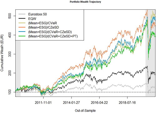
Figure 3 plots the wealth trajectory for the copula-based socially responsible MOOPs. For most out-of-sample periods, the copula-based MOOPs outperform both the EQW and EuroStoxx 50 index. The tri-criteria socially responsible MOOP using CZϵSD as the risk measure performs better than the other strategies before the pandemic crisis. Incorporating all suggested portfolio criteria in the multicriteria reward/risk maximization leads to lower accumulated wealth compared to other MOOPs. This indicates the trade-off between portfolio objectives and accumulated wealth.

To better understand the return-ESG trade-off, we construct and compare socially responsible MOOPs with all five portfolio objectives, while changing the preferences on return (${\lambda }_{\mu }$) and ESG (${\lambda }_{\theta }$). The results reported in Table S2 indicate that increasing the preference on ESG leads to copula-based socially responsible MOOPs with lower average returns. In regard to portfolio risk, the MOOPs with higher ESG preference achieve lower volatility, CVaR, CZϵSD, and average turnover. These results are in accordance with those from Lööf et al. (2021). For instance, when ${\lambda }_{\theta }=90\%,$ the MOOP results in a portfolio strategy with a lower average return (0.038%) as well as lower volatility (1.30%), CVaR (4.81%), and turnover (0.092), compared to the case when ${\lambda }_{\theta }=10\%,$ which results in an average return of 0.071%, volatility of 1.53%, CVaR of 5.30%, and average turnover of 1.07. Furthermore, the MOOPs with higher preference on ESG generally achieve lower CZϵSD than those portfolios with a high preference on returns. Overall, the ESG objective reduces the portfolio’s risk-adjusted performance, e.g. SR and STARR ratios, and accumulated wealth.

In summary, the results in Table 1 indicate (i) the advantages of incorporating multiple objective functions in reward/risk maximization, (ii) a trade-off between the portfolio objectives (e.g. decreasing turnover increases the portfolio CVaR), (iii) that the copula-augmented risk models lead to MOOPs with a higher average return, risk-adjusted performance, and accumulated wealth, however, this comes at the cost of increasing the portfolio risk measures, and (iv) that the ESG objective results in socially responsible MOOPs with lower volatility, CVaR, CZϵSD, and turnover.

5.3. Socially responsible MOOP with individual pillars

In this section, we investigate how socially responsible MOOPs perform when imposing preferences on the individual pillars reflected by environmental (E), social (S), and governance (G) scores. To do so, we construct several copula-based MOOPs with different portfolio objectives. Furthermore, we evaluate MOOPs when all the individual pillars are included as portfolio reward measures, and given the investor’s preferences, several portfolio strategies are constructed.

Table 2 reports the out-of-sample performance for copula-based MOOPs considering the individual pillars. Each panel in Table 2 is comparable to Panel (E) in Table 1. Although the portfolio strategies with individual pillars have similar levels of ESG scores, they have different individual scores depending on their portfolio objectives. For instance, the penta-criteria portfolio in Panel (B) has an ESG score of 79.9% and the highest E score (86.5%), while its counterpart in Panel (D) has the highest G score (84.8%) with a similar ESG score (79.5%). This indicates the possibility of achieving a higher score for individual pillars without a reduction in the overall ESG score. In most cases, the socially responsible MOOPs preferring E scores, in Panel (B), achieve lower volatility and downside risk measured by CVaR, compared to those using S and G pillars. For instance, the penta-criteria portfolio strategy in Panel (B) leads to lower portfolio volatility (1.32%) and CVaR (4.67%), compared to MOOPs in Panel (C) and (D). Interestingly, the MOOPs using S scores achieve a higher average return, risk-adjusted ratios, and accumulated wealth compared to those applying E or G scores. For instance, the tri-criteria MOOP with ${\lambda }_{\mu }=1/2,{\lambda }_S=1/2,{\lambda }_{\zeta }=1$ has the highest average return (0.067%) and Sharpe ratio (0.047). Figure S1 shows that the socially responsible MOOP focusing on the S score achieves higher wealth over the out-of-sample period.

Table 2. Copula-based socially responsible MOOPs with individual pillars.

Portfolio	Ave.	St.
Strategy	Return	Devation	CVaR	CZϵSD	SR	STARR	ESG	E	S	G	Turnover	Wealth
Panel A: Benchmarks
E constrained Max SR	0.030	1.46	5.21	8.88	0.020	0.011	73.4	76.0	72.9	71.3	0.137	172
S constrained Max SR	0.024	1.44	5.18	8.93	0.017	0.009	73.5	75.1	74.3	71.1	0.134	148
G constrained Max SR	0.024	1.40	4.98	8.53	0.017	0.009	73.3	74.9	72.5	73.1	0.143	148
Panel B: Socially responsible MOOPs using E scores
${\lambda }_{\mu }=1/2,{\lambda }_E=1/2,{\lambda }_{\zeta }=1$	0.050	1.35	4.58	7.30	0.037	0.011	79.3	85.4	75.6	76.3	1.30	321
${\lambda }_{\mu }=1/2,{\lambda }_E=1/2,{\lambda }_{\delta }=1$	0.051	1.38	5.26	2.84	0.037	0.010	76.3	79.7	74.6	74.6	1.07	329
${\lambda }_{\mu }=1/2,{\lambda }_E=1/2,{\lambda }_{\zeta }=1/2,{\lambda }_{\delta }=1/2$	0.053	1.35	4.71	5.50	0.039	0.011	78.6	84.2	75.5	75.8	1.26	349
${\lambda }_{\mu }=1/2,{\lambda }_E=1/2,{\lambda }_{\zeta }=1/3,{\lambda }_{\delta }=1/3,{\lambda }_{\vartheta }=1/3$	0.047	1.32	4.67	5.40	0.035	0.010	79.9	86.5	75.7	76.9	0.253	297
Panel C: Socially responsible MOOPs using S scores
${\lambda }_{\mu }=1/2,{\lambda }_S=1/2,{\lambda }_{\zeta }=1$	0.067	1.43	4.76	7.20	0.047	0.014	78.2	76.4	83.2	74.9	1.36	508
${\lambda }_{\mu }=1/2,{\lambda }_S=1/2,{\lambda }_{\delta }=1$	0.053	1.39	5.36	2.72	0.038	0.010	76.4	75.6	78.8	74.9	1.06	347
${\lambda }_{\mu }=1/2,{\lambda }_S=1/2,{\lambda }_{\zeta }=1/2,{\lambda }_{\delta }=1/2$	0.061	1.39	5.01	5.27	0.044	0.012	77.9	76.3	82.2	75.3	1.31	426
${\lambda }_{\mu }=1/2,{\lambda }_S=1/2,{\lambda }_{\zeta }=1/3,{\lambda }_{\delta }=1/3,{\lambda }_{\vartheta }=1/3$	0.055	1.40	5.31	5.14	0.039	0.010	79.2	76.8	84.5	76.3	0.268	362
Panel D: Socially responsible MOOPs using G scores
${\lambda }_{\mu }=1/2,{\lambda }_G=1/2,{\lambda }_{\zeta }=1$	0.045	1.33	4.68	7.16	0.033	0.010	78.4	77.6	75.7	83.4	1.34	276
${\lambda }_{\mu }=1/2,{\lambda }_G=1/2,{\lambda }_{\delta }=1$	0.048	1.38	5.38	2.91	0.035	0.009	76.3	75.9	75.2	79.0	1.05	299
${\lambda }_{\mu }=1/2,{\lambda }_G=1/2,{\lambda }_{\zeta }=1/2,{\lambda }_{\delta }=1/2$	0.050	1.36	4.96	5.37	0.037	0.010	78.2	77.3	76.0	82.8	1.26	316
${\lambda }_{\mu }=1/2,{\lambda }_G=1/2,{\lambda }_{\zeta }=1/3,{\lambda }_{\delta }=1/3,{\lambda }_{\vartheta }=1/3$	0.052	1.35	5.07	5.12	0.039	0.010	79.5	78.4	76.5	84.8	0.249	341

Notes: ${\lambda }_{\mu },{\lambda }_E,{\lambda }_S,{\lambda }_G,{\lambda }_{\zeta },{\lambda }_{\delta },{\lambda }_{\vartheta }$ denote the weights for portfolio return, E, S, G, CVaR, CZϵSD, and turnover, respectively. Portfolio returns are obtained using rolling window estimation (with 500 days as the training sample) and portfolio back-testing from August 18, 2009 until October 7, 2020, resulting in 2853 portfolio out-of-sample net returns using 1 basis point proportional transaction cost. Except for CZϵSD, ESG, and portfolio wealth, all measures are expressed as percentage. CVaR is reported at the 1% level. Accumulated portfolio wealth is calculated at the end of out-of-sample assuming an initial investment of €100. The benchmarks are based on the approach suggested in Pedersen et al. (2021), i.e. maximum Sharpe ratio strategy with boundaries on either environmental (E), social (S), or governance (G) scores.

The suggested MOOP approach allows also to incorporate several reward measures, in particular, when the investor has different preferences on each E, S, and G score. Table S3 reports the out-of-sample performance for socially responsible MOOPs with combined individual pillars. The lowest average return (0.045%) is reported for the MOOP with ${\lambda }_E=40\%,{\lambda }_G=10\%,$ while the highest value (0.059%) is achieved when ${\lambda }_S=30\%,{\lambda }_G=20\%.$ Along with the variations in portfolio risk measures, the results suggest that even small changes, e.g. 10%, in preferences for the individual pillars affect the performance of MOOPs.

Overall the results of this section indicate that (i) using E scores leads to MOOPs with lower risk compared to applying S or G scores and (ii) higher average return and risk-adjusted performance is achieved by MOOPs using S scores.

5.4. MOOP vs MOP approach

To compare the suggested MOOP approach with the MOP using a weighted-sum approach, we simulate step-ahead asset returns from the copula-based risk model. Inserting these returns, we solve the optimization problems (1)(1) $$\begin{array}{cccccc}\hfill & \underset{{\widehat{\mathbf{w}}}_t}{\text{minimize}}\hfill & \hfill & \sum _{q=1}^Q{\lambda }_{{\psi }_q}\left[\frac{{\psi }_q({\widehat{\mathbf{w}}}_t)}{{\underset{¯}{\psi }}_q-{\overline{\psi }}_q}\right]-\hfill & \hfill & \hfill \\ \hfill & \hfill & \hfill & \sum _{k=1}^K{\lambda }_{{\Lambda }_k}\left[\frac{{\Lambda }_k({\widehat{\mathbf{w}}}_t)}{{\overline{\Lambda }}_k-{\underset{¯}{\Lambda }}_k}\right]\hfill & \hfill & \hfill \\ \hfill & \text{subject to}\hfill & \hfill & {\widehat{\mathbf{w}}}_t^{⊺}\mathbf{1}=1\hfill & \hfill & \hfill \\ \hfill & \hfill & \hfill & {\widehat{w}}_{\mathit{\text{jt}}}\ge 0,\forall j\in \{1,2,..,d\}\hfill & \hfill & \hfill \end{array}$$(1) and (5)(5) $$\begin{array}{cccccc}\hfill & \underset{\tilde{\mathbf{w}},\nu ,\tilde{\mathbf{y}},\tilde{\mathbf{g}},\tilde{\mathit{\upsilon }}}{\text{minimize}}\hfill & \hfill & {\lambda }_{{\psi }_{\zeta }}\left[\frac{l+{[M(1-\alpha )]}^{-1}\sum _{m=1}^M{\tilde{\upsilon }}_m}{{\underset{¯}{\Phi }}_{\zeta }^{-1}-{\overline{\Phi }}_{\zeta }^{-1}}\right]+{\lambda }_{{\psi }_{\delta }}\left[\frac{\sum _{m=1}^M{\tilde{y}}_m}{{\underset{¯}{\Phi }}_{\delta }^{-1}-{\overline{\Phi }}_{\delta }^{-1}}\right]+\hfill & \hfill & \hfill \\ \hfill & \hfill & \hfill & {\lambda }_{{\psi }_{\vartheta }}\left[\frac{\sum _{j=1}^d{\tilde{g}}_j}{{\underset{¯}{\Phi }}_{\vartheta }^{-1}-{\overline{\Phi }}_{\vartheta }^{-1}}\right],\hfill & \hfill & \hfill \\ \hfill & \text{subject to}\hfill & \hfill & {\lambda }_{{\Lambda }_{\mu }}{\tilde{\mathbf{w}}}_t^{⊺}{\mathit{\mu }}_t+{\lambda }_{{\Lambda }_{\theta }}{\tilde{\mathbf{w}}}_t^{⊺}{\mathit{\theta }}_t\ge 1,\hfill & \hfill & \hfill \\ \hfill & \hfill & \hfill & {\tilde{y}}_m+{\tilde{\mathbf{w}}}_t^{⊺}{\widehat{\mathbf{r}}}_{\mathit{\text{mt}}}\ge \nu r_{\mathit{\text{mt}}}^I,\hfill & \hfill & \forall m\in \{1,2,..,M\},\hfill \\ \hfill & \hfill & \hfill & -{\tilde{\mathbf{w}}}_t^{⊺}{\widehat{\mathbf{r}}}_{\mathit{\text{mt}}}+l+{\tilde{\upsilon }}_m\ge 0,\hfill & \hfill & \forall m\in \{1,2,..,M\},\hfill \\ \hfill & \hfill & \hfill & {\tilde{\upsilon }}_m\ge 0,\hfill & \hfill & \forall m\in \{1,2,..,M\},\hfill \\ \hfill & \hfill & \hfill & {\tilde{w}}_{\mathit{\text{jt}}}+{\tilde{g}}_j\ge \nu {\widehat{w}}_{j{t}^{*}},\hfill & \hfill & \forall j\in \{1,2,..,d\},\hfill \\ \hfill & \hfill & \hfill & {\tilde{g}}_j-{\tilde{w}}_{\mathit{\text{jt}}}\ge -\nu {\widehat{w}}_{j{t}^{*}},\hfill & \hfill & \forall j\in \{1,2,..,d\},\hfill \\ \hfill & \hfill & \hfill & {\tilde{\mathbf{w}}}_t^{⊺}\mathbf{1}=\nu ,\hfill & \hfill & \hfill \\ \hfill & \hfill & \hfill & 0\le {\tilde{w}}_{\mathit{\text{jt}}}\le \nu \hfill & \hfill & \forall j\in \{1,2,..,d\},\hfill \\ \hfill & \hfill & \hfill & \nu >0,\hfill & \hfill & \hfill \end{array}$$(5) for all out-of-sample iterations and plot the value of the multicriteria reward/risk ratio, i.e. $({\mu }_t+{\theta }_t)/({\zeta }_t+{\vartheta }_t+{\delta }_t).$ This procedure corresponds to Steps 1–8 in Section 3. Figure 2 provides the results. For the MOP approach, the green line includes the reward/risk ratios using equal weights for all five objective functions, while the red line plots these ratios applying equal weights to the reward measures (summing up to 50%) and equal weights to the risk measures (summing up to 50%). For most out-of-sample iterations, the MOOP optimization provides higher values for the objective function (blue line) than its MOP counterparts. This indicates the advantage of the suggested MOOP approach in finding solutions with higher multicriteria ratios.

Figure 2. The value of the objective function includes the reward/risk ratio, $({\mu }_t+{\theta }_t)/({\zeta }_t+{\vartheta }_t+{\delta }_t).$ The portfolio optimizations are based on all stocks included in EuroStoxx 50 index from August 18, 2009 until October 7, 2020.

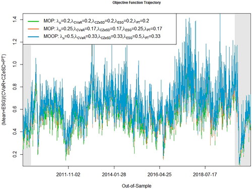
Figure 3. This figure plots the wealth accumulation trajectory for the copula-based socially responsible MOOPs. The portfolio optimizations are based on all stocks included in EuroStoxx 50 index from December 8, 2016 to October 7, 2020.

To compare the out-of-sample performance of the two approaches, we estimate the penta-criteria socially responsible MOPs with different preferences on portfolio return and ESG. We consider the MOPs where the total weights for reward measures are 50%, with equal weights on the risk measures. Table S4 presents the results. In comparison to the results in Table S2, in most cases, the socially responsible MOOPs achieve higher expected returns as well as lower volatility and CVaR. For instance, the socially responsible MOOP with ${\lambda }_{\mu }=90\%,{\lambda }_{\theta }=10\%$ results in higher portfolio return (0.071%) and lower CVaR (5.30%) and CZϵSD (7.33) compared to its MOP counterpart with ${\lambda }_{\mu }=45\%,{\lambda }_{\theta }=5\%.$ When imposing more weights on portfolios’ ESG score, the socially responsible MOOPs achieve slightly higher ESG at the cost of higher CZϵSD and turnover compared to the socially responsible MOPS. For instance, the socially responsible MOP with ${\lambda }_{\mu }=10\%,{\lambda }_{\theta }=40\%$ leads to lower CZϵSD (4.65) compared to the value (5.00) achieved by the socially responsible MOOP with ${\lambda }_{\mu }=20\%,{\lambda }_{\theta }=80\%.$ These results indicate that the MOOP approach does not always provide higher rewards and less risk than those from the MOP optimization. In some cases, the out-performance in terms of some of the objective functions leads to under-performance in others.

6. Conclusions

This article suggests a multiobjective reward/risk maximization of a portfolio problem that is based on the common weighted-sum approach and linear fractional programming. The suggested approach enables the estimation of multiobjective optimal portfolios and narrows down the investor choices to reward/risk portfolios while allowing a weighting scheme for multiple objectives.

The results support the suggested MOOP portfolio approach and indicate the advantages of incorporating multiple objective functions in reward/risk maximization. However, there is a trade-off between reward and risk measures. The copula-augmented risk models lead to MOOPs with higher average return, risk-adjusted performance, and accumulated wealth compared to the historical approach, but this comes at the cost of increasing the portfolio risk measures. Applying the ESG objective results in socially responsible MOOPs with lower volatility, CVaR, CZϵSD, and turnover. In other words, considering social responsibility for portfolio construction results in lower portfolio return as well as in lower risk-adjusted return and accumulated wealth, but on the other hand portfolio risk is also reduced. Comparing the individual ESG pillars, optimizing environmental scores leads to less risky MOOPs, while optimizing social scores results in higher average return and risk-adjusted performance.

Acknowledgment

We are grateful to Claudia Czado, Richard Harris, Ranadeva Jayasekera, and Victor Troster for their helpful comments on a previous version of this article. In addition, we are grateful to seminar participants at the ETH Zurich, the 14th International Conference on Computational and Financial Econometrics (London, 2020), 3rd Symposium of the Emerging Topics in Financial Economics (Sweden, 2021), 1st Conference on International Finance; Sustainable and Climate Finance and Growth (Italy, 2022). Some of the computations for this study were done using the R packages” rmgarch”, and” rvinecopulib” (Ghalanos, 2019; Nagler & Vatter, 2021). The usual disclaimer applies.

Disclosure statement

No potential conflict of interest was reported by the authors.

Notes

1 Notice in a multiobjective setting, the nadir solutions are defined using the Pareto optimal solutions. However, we approximate these solutions using a set of feasible solutions obtained from separate optimizations of each objective (reward/risk) functions in the MOP (MOOP) approach.

References

- Aouni, B., Doumpos, M., Pérez-Gladish, B., & Steuer, R. E. (2018). On the increasing importance of multiple criteria decision aid methods for portfolio selection. Journal of the Operational Research Society, 69(10), 1525–1542. https://doi.org/10.1080/01605682.2018.1475118
- Ballestero, E., Bravo, M., Pérez-Gladish, B., Arenas-Parra, M., & Plà-Santamaria, D. (2012). Socially responsible investment: A multicriteria approach to portfolio selection combining ethical and financial objectives. European Journal of Operational Research, 216(2), 487–494. https://doi.org/10.1016/j.ejor.2011.07.011
- Ballestero, E., & Romero, C. (1996). Portfolio selection: A compromise programming solution. Journal of the Operational Research Society, 47(11), 1377–1386. https://doi.org/10.2307/3010203
- Bilbao, A., Arenas, M., Jiménez, M., Perez Gladish, B., & Rodríguez, M. (2006). An extension of sharpe’s single-index model: Portfolio selection with expert betas. Journal of the Operational Research Society, 57(12), 1442–1451. https://doi.org/10.1057/palgrave.jors.2602133
- Bilbao-Terol, A., Arenas-Parra, M., Cañal-Fernández, V., & Jiménez, M. (2016). A sequential goal programming model with fuzzy hierarchies to sustainable and responsible portfolio selection problem. Journal of the Operational Research Society, 67(10), 1259–1273. https://doi.org/10.1057/jors.2016.33
- Bruni, R., Cesarone, F., Scozzari, A., & Tardella, F. (2017). On exact and approximate stochastic dominance strategies for portfolio selection. European Journal of Operational Research, 259(1), 322–329. https://doi.org/10.1016/j.ejor.2016.10.006
- Cao, Y., Fuentes-Cortes, L. F., Chen, S., & Zavala, V. M. (2017). Scalable modeling and solution of stochastic multiobjective optimization problems. Computers & Chemical Engineering, 99, 185–197. https://doi.org/10.1016/j.compchemeng.2017.01.021
- Charnes, A., & Cooper, W. W. (1962). Programming with linear fractional functionals. Naval Research Logistics Quarterly, 9(3–4), 181–186. https://doi.org/10.1002/nav.3800090303
- Dinkelbach, W. (1967). On nonlinear fractional programming. Management Science, 13(7), 492–498. https://doi.org/10.1287/mnsc.13.7.492
- Gasser, S. M., Rammerstorfer, M., & Weinmayer, K. (2017). Markowitz revisited: Social portfolio engineering. European Journal of Operational Research, 258(3), 1181–1190. https://doi.org/10.1016/j.ejor.2016.10.043
- Ghalanos, A. (2019). rmgarch: Multivariate GARCH Models. URL: https://cran.r-project.org/package=rmgarch R package version 1.3-7.
- Goel, A., & Sharma, A. (2021). Deviation measure in second-order stochastic dominance with an application to enhanced indexing. International Transactions in Operational Research, 28(4), 2218–2247. https://doi.org/10.1111/itor.12629
- Henriques, C. O., & Neves, M. E. D. (2019). A multiobjective interval portfolio framework for supporting investor’s preferences under different risk assumptions. Journal of the Operational Research Society, 70(10), 1639–1661. https://doi.org/10.1080/01605682.2019.1571004
- Hirschberger, M., Steuer, R. E., Utz, S., Wimmer, M., & Qi, Y. (2013). Computing the nondominated surface in tri-criterion portfolio selection. Operations Research, 61(1), 169–183. https://doi.org/10.1287/opre.1120.1140
- Lindquist, W. B., Rachev, S. T., Hu, Y., & Shirvani, A. (2022). Inclusion of esg ratings in optimization. In Advanced REIT Portfolio Optimization: Innovative Tools for Risk Management. (pp. 227–245). Springer International Publishing. URL. https://doi.org/10.1007/978-3-031-15286-3_13.
- Lööf, H., Sahamkhadam, M., & Stephan, A. (2021). Is corporate social responsibility investing a free lunch? the relationship between ESG, tail risk, and upside potential of stocks before and during the covid-19 crisis. Finance Research Letters, 46, 102499. https://doi.org/10.1016/j.frl.2021.102499
- Lööf, H., Sahamkhadam, M., & Stephan, A. (2023). Incorporating ESG into optimal stock portfolios for the global timber & forestry industry. Journal of Forest Economics, 38(2), 133–157. https://doi.org/10.1561/112.00000560
- Martel, J.-M., Khoury, N., & Bergeron, M. (1988). An application of a multicriteria approach to portfolio comparisons. Journal of the Operational Research Society, 39(7), 617–628. https://doi.org/10.1057/jors.1988.107
- Masmoudi, M., & Abdelaziz, F. B. (2018). Portfolio selection problem: A review of deterministic and stochastic multiple objective programming models. Annals of Operations Research, 267(1–2), 335–352. https://doi.org/10.1007/s10479-017-2466-7
- Nagler, T., Bumann, C., & Czado, C. (2019). Model selection in sparse high-dimensional vine copula models with an application to portfolio risk. Journal of Multivariate Analysis, 172, 180–192. https://doi.org/10.1016/j.jmva.2019.03.004
- Nagler, T., Vatter, T. (2021). rvinecopulib: High Performance Algorithms for Vine Copula Modeling. URL: https://cran.r-project.org/package=rvinecopulib R package version 0.5.5.1.1.
- Pedersen, L. H., Fitzgibbons, S., & Pomorski, L. (2021). Responsible investing: The ESG-efficient frontier. Journal of Financial Economics, 142(2), 572–597. https://doi.org/10.1016/j.jfineco.2020.11.001
- Roman, D., Mitra, G., & Zverovich, V. (2013). Enhanced indexation based on second-order stochastic dominance. European Journal of Operational Research, 228(1), 273–281. https://doi.org/10.1016/j.ejor.2013.01.035
- Sahamkhadam, M., Stephan, A., & Östermark, R. (2022). Copula-based black–litterman portfolio optimization. European Journal of Operational Research, 297(3), 1055–1070. https://doi.org/10.1016/j.ejor.2021.06.015
- Sharma, A., Agrawal, S., & Mehra, A. (2017). Enhanced indexing for risk averse investors using relaxed second order stochastic dominance. Optimization and Engineering, 18(2), 407–442. https://doi.org/10.1007/s11081-016-9329-y
- Steuer, R. E. (1986). Multiple criteria optimization: Theory, computation and applications. Wiley.
- Steuer, R. E., & Utz, S. (2023). Non-contour efficient fronts for identifying most preferred portfolios in sustainability investing. European Journal of Operational Research, 306(2), 742–753. https://doi.org/10.1016/j.ejor.2022.08.007
- Stoyanov, S. V., Rachev, S. T., & Fabozzi, F. J. (2007). Optimal financial portfolios. Applied Mathematical Finance, 14(5), 401–436. https://doi.org/10.1080/13504860701255292
- Utz, S., Wimmer, M., Hirschberger, M., & Steuer, R. E. (2014). Tri-criterion inverse portfolio optimization with application to socially responsible mutual funds. European Journal of Operational Research, 234(2), 491–498. https://doi.org/10.1016/j.ejor.2013.07.024
- Utz, S., Wimmer, M., & Steuer, R. E. (2015). Tri-criterion modeling for constructing more-sustainable mutual funds. European Journal of Operational Research, 246(1), 331–338. https://doi.org/10.1016/j.ejor.2015.04.035
- Xidonas, P., Mavrotas, G., Hassapis, C., & Zopounidis, C. (2017). Robust multiobjective portfolio optimization: A minimax regret approach. European Journal of Operational Research, 262(1), 299–305. https://doi.org/10.1016/j.ejor.2017.03.041
- Xidonas, P., Mavrotas, G., Krintas, T., Psarras, J., & Zopounidis, C. (2012). Multicriteria portfolio management. In Multicriteria Portfolio Management (pp. 5–21). Springer.