Full article: A novel strong duality-based reformulation for trilevel infrastructure models in energy systems development

Formulae display: $MathJax Logo$ ?Mathematical formulae have been encoded as MathML and are displayed in this HTML version using MathJax in order to improve their display. Uncheck the box to turn MathJax off. This feature requires Javascript. Click on a formula to zoom.

Abstract

We explore the class of trilevel equilibrium problems with a focus on energy-environmental applications and present a novel single-level reformulation for such problems, based on strong duality. To the best of our knowledge, only one alternative single-level reformulation for trilevel problems exists. This reformulation uses a representation of the bottom-level solution set, whereas we propose a reformulation based on strong duality. Our novel reformulation is compared to this existing formulation, discussing both model sizes and computational performance. In particular, we apply this trilevel framework to a power market model, exploring the possibilities of an international policymaker in reducing emissions of the system. Using the proposed approach, we are able to obtain globally optimal solutions for a five-node case study representing the Nordic countries and assess the impact of a carbon tax on the electricity production portfolio.

Keywords:

1. Introduction

Hierarchical optimisation models with three levels of decision-makers arise in contexts such as traffic equilibrium (Gabriel, et al., Citation2022; Gu et al., Citation2019) and electricity market modelling (Huppmann and Egerer, Citation2015; Jin and Ryan, Citation2014). The hierarchical structure can be, e.g., such that the bottom-level players use a network operated by a middle-level player and regulated by a top-level player. For both electricity and traffic networks, similar models without the top-level regulators have been explored using bilevel optimisation, see Sinha et al. (Citation2018) for a review.

Albeit challenging from both methodological and computational standpoints, including a top-level regulator as the third level, as opposed to considering only bilevel models, can provide important policy insights. In the particular case of energy systems, these models can yield more realistic solutions in which more stakeholders are assumed to act in coordination considering their own objectives. Obtaining equilibrium solutions for these models can thereby provide policy insights on pathways towards decarbonisation goals. Gabriel, et al. (Citation2022) present a single-level reformulation for bilevel problems with complementarity-constrained bottom levels and discuss the possibility of using the model in a trilevel power market setting. However, their article includes no computational experiments demonstrating the practical usability of the proposed methods. Our aim is to explore the computational efficiency of the method using an illustrative power system setting representing the market structure in the Nordic countries.

The contribution of this article is twofold. First, in Section 2, we present background on bi- and tri-level optimisation, ending with our novel approach for solving trilevel equilibrium problems based on strong duality in Section 2.4. Compared to the formulation presented in Gabriel, et al. (Citation2022) and summarised in Section 2.3, our proposed formulation results in fewer constraints, which is likely to result in increased computational efficiency. Second, we illustrate the methodological contributions using a stylised trilevel power market model described in Section 3. The motivation for our application stems from the recent discussion about optimal carbon taxation and its impact on electricity production (e.g., Hájek et al., Citation2019). The computational performance of the model is explored in Section 4.1, and finally, in Section 4.2, we apply the trilevel equilibrium modelling framework to a power market case study based on Belyak et al. (Citation2023). These contributions are significant for the novel class of trilevel optimisation problems, and equilibrium modelling area in general. Finally, Section 5 concludes the article and discusses future research directions.

2. Background

2.1. Earlier research

Bilevel optimisation considers problems with a hierarchical structure consisting of an upper-level player and one or more lower-level players (Bard, Citation1983). In power sector models (Gabriel, et al., Citation2012), the upper-level player is often a transmission system operator and the bottom level consists of electricity producers in a Cournot oligopoly. The general structure of a bilevel problem with linear upper- and lower-level problems is presented in Equation(1)(1a) $(P_{u}) : mi n_{x, y \geq 0} c_{1}^{⊤} x + d_{1}^{⊤} y$ (1a) and Equation(2)(2a) $(P_{l} (x)) : mi n_{y \geq 0} d_{2}^{⊤} y$ (2a) . The upper-level problem P_u is (1a) $(P_{u}) : mi n_{x, y \geq 0} c_{1}^{⊤} x + d_{1}^{⊤} y$ (1a) (1b) $s . t . A_{1} x + B_{1} y \geq a_{1},$ (1b) (1c) $y solves P_{l} (x),$ (1c) where $P_{l} (x)$ denotes the lower-level problem. Here, $c_{1}, x \in R^{n_{x}}, d_{1}, y \in R^{n_{y}}, A_{1} \in R^{m_{u} \times n_{x}}, B_{1} \in R^{m_{u} \times n_{y}},$ and $a_{1} \in R^{m_{u}} .$ The overall idea of this formulation is that the upper-level player’s decision variable x affects the lower-level players’ optimal decisions y, which is reflected back to the upper level in the constraint Equation(1c)(1c) $y solves P_{l} (x),$ (1c) . The linear lower-level problem is formulated as (2a) $(P_{l} (x)) : mi n_{y \geq 0} d_{2}^{⊤} y$ (2a) (2b) $s . t . A_{2} x + B_{2} y \geq a_{2} .$ (2b)

In general, both problems can also include equality constraints, but they have been omitted here for brevity, without loss of generality.

Solution methods for bilevel problems are based on the idea of replacing the upper-level constraint Equation(1c)(1c) $y solves P_{l} (x),$ (1c) with the optimality conditions of the lower-level problem Equation(2)(2a) $(P_{l} (x)) : mi n_{y \geq 0} d_{2}^{⊤} y$ (2a) . The two main alternatives are the Karush–Kuhn–Tucker (KKT) optimality conditions (Karush, Citation1939; Kuhn and Tucker, Citation1951), leading to a mathematical program with equilibrium constraints (MPEC); and mathematical programming with primal and dual constraints (MPPDC) (Baringo and Conejo, Citation2012; Ruiz et al., Citation2012). Additionally, approaches based on optimal value functions (Ye and Zhu, Citation1995) can be used. Bilevel optimisation models can be used in contexts such as Stackelberg games (Bard, Citation1991), Cournot competition (Gabriel, et al., Citation2012), and robust optimisation (Leyffer et al., Citation2020). For a recent survey on applications and algorithms for bilevel optimisation, we refer to Kleinert et al. (Citation2021).

A major challenge in bilevel optimisation is that, even for linear bilevel problems, single-level reformulations using complementarity constraints lead to non-linear and non-convex problems. This significantly increases the computational complexity of solving such problems and requires specialised approaches such as the simplex method-inspired projected gradient method by Still (Citation2002) or the (spatial) branch-and-bound methods discussed by Bard and Moore (Citation1990) and implemented in the Gurobi solver (Gurobi Optimization, LLC, Citation2022). Alternatively, one can use heuristics such as genetic programming (Kieffer et al., Citation2020) and particle swarm optimisation (Gao and Liu, Citation2021). For a review on heuristic solution methods for bilevel programming, we refer the reader to Camacho-Vallejo et al. (Citation2023).

2.2. Trilevel equilibrium models

Consider a problem with a trilevel structure, in which players interact with each other at all three levels: top, middle, and bottom. In this structure, the top-level problem P₁ is assumed to be a linear optimisation problem with the middle-level problem $P_{2} (x)$ represented by the constraint Equation(3c)(3c) $y, z solve P_{2} (x),$ (3c) . (3a) $(P_{1}) : mi n_{x, y, z} c_{1}^{⊤} x + d_{1}^{⊤} y + e_{1}^{⊤} z$ (3a) (3b) $s . t . A_{1} x + B_{1} y + C_{1} z \geq a_{1}$ (3b) (3c) $y, z solve P_{2} (x),$ (3c) where $P_{2} (x)$ denotes the middle-level problem (4a) $(P_{2} (x)) : mi n_{y, z} d_{2}^{⊤} y + e_{2}^{⊤} z$ (4a) (4b) $s . t . A_{2} x + B_{2} y + C_{2} z \geq a_{2} (γ)$ (4b) (4c) $y \geq 0$ (4c) (4d) $z solves P_{3} (x, y),$ (4d) where γ is the vector of dual variables associated with constraint Equation(4b)(4b) $s . t . A_{2} x + B_{2} y + C_{2} z \geq a_{2} (γ)$ (4b) and z is the vector of bottom-level variables. In trilevel settings, the “lower-level” problem $P_{2} (x)$ is itself a bilevel problem. This is challenging, because bilevel optimisation problems are generally non-convex and directly obtaining their optimality conditions is thus difficult. The middle-level problem $P_{2} (x)$ constraints contain a bottom-level problem $P_{3} (x, y)$ that is parameterised by the upper-level variables x and middle-level variables y. In particular, Gabriel, et al. (Citation2022) discuss the case of the bottom-level problem being a linear complementarity problem (LCP) (5) $P_{3} (x, y) : 0 \leq \tilde{z} ⊥ q + N_{x} x + N_{y} y + M \tilde{z} \geq 0$ (5) parameterised via the vector terms $N_{x} x$ and $N_{y} y .$ It should be noted that Equation(5)(5) $P_{3} (x, y) : 0 \leq \tilde{z} ⊥ q + N_{x} x + N_{y} y + M \tilde{z} \geq 0$ (5) can be viewed as the KKT conditions of convex quadratic problems and in Section 2.4, we discuss such problems in more detail. Hereinafter, we use the standard $⊥$ -notation $0 \leq a ⊥ b \geq 0 \Leftrightarrow a, b \geq 0, a^{⊤} b = 0$ for complementarity constraints with vectors a and b.

Trilevel problems have been researched by, e.g., Sauma and Oren (Citation2007), who do not solve the models directly and instead iteratively solve the middle- and bottom-level problems for different values of the top-level decision variables, and Dvorkin et al. (Citation2018), who employ a column-and-constraint generation algorithm. In contrast, the goal of this article is to explore novel single-level reformulations for trilevel problems and solve them using an off-the-shelf solver, thus lowering the barrier-to-entry for using these models. However, this comes at the expense of imposing constraints on the structure of the models that are tractable in this manner. In Equation(4)(4a) $(P_{2} (x)) : mi n_{y, z} d_{2}^{⊤} y + e_{2}^{⊤} z$ (4a) , a general form of the problem is used, and the bottom-level problem in Equation(4d)(4d) $z solves P_{3} (x, y),$ (4d) is assumed to be parameterised by both x and y. For the sake of clarity, we define two classes of trilevel problems with different degrees of computational challenges.

Definition 2.1.

If P₃ is parameterised by both x and y, we say that the problem has a strong trilevel structure. In contrast, if P₃ is parameterised only by the top-level variables x, i.e., it is not directly dependent on y, we say that the problem has a weak trilevel structure.

Gabriel, et al. (Citation2022) show that in order to use their single-level reformulation, the problem must have a weak trilevel structure, allowing such problems to be solved rather effectively by borrowing from the results in Cottle et al. (Citation2009, Theorem 3.1.6) as long as the matrix M in the lower-level problem Equation(5)(5) $P_{3} (x, y) : 0 \leq \tilde{z} ⊥ q + N_{x} x + N_{y} y + M \tilde{z} \geq 0$ (5) is positive semi-definite (PSD). We also show that our novel reformulation in Section 2.4 retains this structural limitation and that the energy-environmental planning problem considered in this article has this structure. The aim of this article is to develop an alternative reformulation improving computational tractability and efficiency compared to the reformulation in Gabriel, et al. (Citation2022), and the discussion on ways for lifting this restriction on problem structure is outside the scope of this article.

While the lack of direct influence for the middle-level player is a limitation, there are still structures that necessitate the use of a trilevel framework. As an example of a setting where a trilevel approach is required, we use the power market example in Section 3, where the bottom level consists of electricity generators, and on the middle level we have a profit-maximising system operator who has to satisfy a minimum renewable share in electricity production. If the bottom-level LCP matrix M in Equation(5)(5) $P_{3} (x, y) : 0 \leq \tilde{z} ⊥ q + N_{x} x + N_{y} y + M \tilde{z} \geq 0$ (5) is PSD, the bottom-level problem can have multiple optima. This could result in, e.g., a situation where it makes no difference for a generator to produce electricity using coal in one node or wind power in another.

Using the optimistic bilevel assumption (Dempe and Zemkoho, Citation2020), while the system operator cannot directly influence the generators, they can choose a bottom-level optimum that maximises their profit while satisfying the minimum renewable share constraint. In turn, maximising the middle-level player’s profit could, in some settings, result in worse objective values for the top-level player. These interactions could not be represented in a setting where the middle-level player is insensitive to the bottom-level player’s decisions, as the middle-level player must consider the bottom-level optimality conditions to be able to choose between bottom-level optimal solutions.

2.3. Bottom-level LCP with a positive semi-definite coefficient matrix

For completeness, we summarise the solution approach introduced in Gabriel, et al. (Citation2022). Let us assume that the matrix M in Equation(5)(5) $P_{3} (x, y) : 0 \leq \tilde{z} ⊥ q + N_{x} x + N_{y} y + M \tilde{z} \geq 0$ (5) is PSD and that we have a solution $\bar{z}$ of Equation(5)(5) $P_{3} (x, y) : 0 \leq \tilde{z} ⊥ q + N_{x} x + N_{y} y + M \tilde{z} \geq 0$ (5) . Furthermore, we assume the problem to have a weak trilevel structure and thus N_y = 0, i.e., the middle-level decisions y do not influence the bottom-level problem (c.f. Definition 2.1). Gabriel, et al. (Citation2022) show that for a PSD M and a weak trilevel structure, a solution to the trilevel problem consisting of Equation(3)(3a) $(P_{1}) : mi n_{x, y, z} c_{1}^{⊤} x + d_{1}^{⊤} y + e_{1}^{⊤} z$ (3a) –Equation(5)(5) $P_{3} (x, y) : 0 \leq \tilde{z} ⊥ q + N_{x} x + N_{y} y + M \tilde{z} \geq 0$ (5) can be obtained by solving the equivalent single-level reformulation (6a) $min_{x, y, \tilde{z}, \bar{z}, β, γ, δ, ζ, η} c_{1}^{⊤} x + d_{1}^{⊤} y + e_{1}^{⊤} \tilde{z}$ (6a) (6b) $s . t . A_{1} x + B_{1} y + C_{1} \tilde{z} \geq a_{1},$ (6b) (6c) $0 \leq y ⊥ d_{2} - B_{2}^{⊤} γ \geq 0,$ (6c) (6d) $0 \leq \tilde{z} ⊥ e_{2} - C_{2}^{⊤} γ - M^{⊤} δ - ζ (q + N_{x} x) - {(M + M^{⊤})}^{⊤} η \geq 0,$ (6d) (6e) $0 \leq \bar{z} ⊥ q + N_{x} x + (M + M^{⊤}) \bar{z} - M^{⊤} β \geq 0,$ (6e) (6f) $0 \leq β ⊥ q + N_{x} x + M \bar{z} \geq 0,$ (6f) (6g) $0 \leq δ ⊥ (q + N_{x} x) + M \tilde{z} \geq 0,$ (6g) (6h) ${(q + N_{x} x)}^{⊤} (\tilde{z} - \bar{z}) = 0, (M + M^{⊤}) (\tilde{z} - \bar{z}) = 0,$ (6h) (6i) $0 \leq γ ⊥ A_{2} x + B_{2} y + C_{2} \tilde{z} - a_{2} \geq 0,$ (6i) where $\bar{z}$ is a solution to the bottom-level problem Equation(5)(5) $P_{3} (x, y) : 0 \leq \tilde{z} ⊥ q + N_{x} x + N_{y} y + M \tilde{z} \geq 0$ (5) and ${({\bar{z}}^{*})}^{⊤} (q + N_{x} x^{*} + M {\bar{z}}^{*}) = 0$ has to thus hold at an optimal solution $x^{*}, {\bar{z}}^{*}$ to Equation(6)(6a) $min_{x, y, \tilde{z}, \bar{z}, β, γ, δ, ζ, η} c_{1}^{⊤} x + d_{1}^{⊤} y + e_{1}^{⊤} \tilde{z}$ (6a) . Appendix A summarises the reformulation steps taken in Gabriel, et al. (Citation2022), including the constraints corresponding to the dual variables $β, δ, ζ,$ and η. This formulation assumes non-negativity for all variables y, but we note that this is not a requirement and including free variables in the middle level only requires small changes to the corresponding KKT conditions Equation(6c)(6c) $0 \leq y ⊥ d_{2} - B_{2}^{⊤} γ \geq 0,$ (6c) .

Finally, we note that the reformulation Equation(6)(6a) $min_{x, y, \tilde{z}, \bar{z}, β, γ, δ, ζ, η} c_{1}^{⊤} x + d_{1}^{⊤} y + e_{1}^{⊤} \tilde{z}$ (6a) is not linear due to the non-linear products $ζ N_{x} x, x^{⊤} N_{x}^{⊤} \tilde{z}$ and $x^{⊤} N_{x}^{⊤} \bar{z},$ resulting in a non-convex problem. In general, obtaining global optimal solutions to non-convex problems is enormously challenging, but this particular non-convexity can be handled by using a solver capable of handling problems with bilinear terms in special ordered sets of type 1 (SOS1) constraints (Beale and Tomlin, Citation1970). An SOS1 constraint states that out of a set of variables or functions, only one can have a non-zero value. A complementarity constraint $0 \leq a ⊥ b \geq 0$ can thus be reformulated as two non-negative variables a and b in an SOS1 constraint. This can be achieved using, e.g., the spatial branch-and-bound method in the Gurobi solver (Gurobi Optimization, LLC, Citation2022); see also Siddiqui and Gabriel (Citation2013).

2.4. Mathematical programming with complementarity from primal and dual constraints

We are now ready to discuss our novel single-level reformulation. Let us first consider a setting where the bottom level is a convex quadratic minimisation problem. So far, we have discussed a reformulation based on adding the KKT optimality conditions of the bottom-level problem to the middle-level problem. In our trilevel case, the KKT optimality conditions, having complementarity constraints, require a reformulation of the LCP solution set so that we can obtain a single-level equivalent formulation of the trilevel problem. This eventually results in the middle- and bottom-level problems being represented as two optimisation problems, potentially leading to computational challenges with the reformulation Equation(6)(6a) $min_{x, y, \tilde{z}, \bar{z}, β, γ, δ, ζ, η} c_{1}^{⊤} x + d_{1}^{⊤} y + e_{1}^{⊤} \tilde{z}$ (6a) . Representing these two nested optimisation problems as a single-level equivalent requires a large number of complementarity constraints Equation(6e)(6e) $0 \leq \bar{z} ⊥ q + N_{x} x + (M + M^{⊤}) \bar{z} - M^{⊤} β \geq 0,$ (6e) –Equation(6i)(6i) $0 \leq γ ⊥ A_{2} x + B_{2} y + C_{2} \tilde{z} - a_{2} \geq 0,$ (6i) , possibly leading to prohibitive computational requirements.

To circumvent these challenges, we note that some bilevel optimisation problems can also be reformulated as MPPDC, using strong duality instead of complementarity. We present a novel strong duality-based reformulation for trilevel problems, in which a linear middle-level problem and convex quadratic bottom-level problems are reformulated into a single quadratically constrained linear problem instead of two optimisation problems (a quadratic program (QP) and a linear program (LP)) as in Appendix A and Gabriel, et al. (Citation2022). The model sizes resulting from using complementarity (Section 2.3) and strong duality (this section) for the bottom level are compared in Section 2.5.

Consider a trilevel problem with a set of bottom-level problems $P_{3 i} (x)$ (7a) $(P_{3 i} (x)) : min_{z_{i}} \frac{1}{2} z_{i}^{⊤} F_{i} z_{i} + e_{i 3} {(x)}^{⊤} z_{i}$ (7a) (7b) $s . t . C_{i 3} z_{i} \geq a_{i 3} (x)$ (7b) (7c) $z_{i} \geq 0,$ (7c) where z_i is a vector of decision variables and F_i is PSD for all $i \in I .$ In our illustrative example described in the next section, the set I represents the electricity producers. Note that we assume a weak trilevel structure, that is, $P_{3 i}$ does not depend on y. Dorn (Citation1960) presents Lagrangian dual formulations for quadratic problems,Footnote¹ and using these formulations, the dual of each problem $P_{3 i} (x)$ is (8a) $max_{p_{i}, z_{i}} - \frac{1}{2} z_{i}^{⊤} F_{i} z_{i} + a_{i 3} {(x)}^{⊤} p_{i}$ (8a) (8b) $s . t . C_{i 3}^{⊤} p_{i} - F_{i} z_{i} \leq e_{i 3} (x)$ (8b) (8c) $p_{i} \geq 0.$ (8c)

In MPPDC, the complementarity constraints in the KKT optimality conditions are replaced with a strong duality constraint. The strong duality theorem (e.g., Bazaraa et al., Citation2013) states that if the problem has no duality gap, that is, some constraint qualification holds for the problem,Footnote² The optimal primal and dual objective values are equal. This implies that such problems can be solved to optimality by finding any solution that is both primal and dual feasible with the primal and dual objective values being equal.

Combining formulations Equation(7)(7a) $(P_{3 i} (x)) : min_{z_{i}} \frac{1}{2} z_{i}^{⊤} F_{i} z_{i} + e_{i 3} {(x)}^{⊤} z_{i}$ (7a) and Equation(8)(8a) $max_{p_{i}, z_{i}} - \frac{1}{2} z_{i}^{⊤} F_{i} z_{i} + a_{i 3} {(x)}^{⊤} p_{i}$ (8a) , we obtain the following primal and dual constraints, combined with a strong-duality constraint: (9a) $C_{i 3} z_{i} \geq a_{i 3} (x) \forall i \in I$ (9a) (9b) $C_{i 3}^{⊤} p_{i} - F_{i} z_{i} \leq e_{i 3} (x) \forall i \in I$ (9b) (9c) $z_{i}^{⊤} F_{i} z_{i} + e_{i 3} {(x)}^{⊤} z_{i} - a_{i 3} {(x)}^{⊤} p_{i} \leq 0 \forall i \in I$ (9c) (9d) $z_{i}, p_{i} \geq 0 \forall i \in I .$ (9d)

The strong duality constraint Equation(9c)(9c) $z_{i}^{⊤} F_{i} z_{i} + e_{i 3} {(x)}^{⊤} z_{i} - a_{i 3} {(x)}^{⊤} p_{i} \leq 0 \forall i \in I$ (9c) states that the objective value of each bottom-level primal (minimisation) problem must not be higher than the value of the dual (maximisation) problem. Recall that the weak duality theorem (Bazaraa et al., Citation2013) states that the objective value of any solution of a minimisation problem is greater or equal to any objective value of the corresponding dual problem. This result allows us to write the strong duality constraint in an inequality form, following the approach in Huppmann and Egerer (Citation2015), thus avoiding a quadratic equality constraint that would render a non-convex feasible region. Since the matrices F_i are PSD, constraints Equation(9c)(9c) $z_{i}^{⊤} F_{i} z_{i} + e_{i 3} {(x)}^{⊤} z_{i} - a_{i 3} {(x)}^{⊤} p_{i} \leq 0 \forall i \in I$ (9c) are convex. Knowing that weak duality guarantees the left-hand side of each constraint Equation(9c)(9c) $z_{i}^{⊤} F_{i} z_{i} + e_{i 3} {(x)}^{⊤} z_{i} - a_{i 3} {(x)}^{⊤} p_{i} \leq 0 \forall i \in I$ (9c) to be non-negative also allows us to combine the $| I |$ constraints into one by taking a sum over the left-hand side values, reducing the number of constraints.

By combining the middle-level problem Equation(4a)(4a) $(P_{2} (x)) : mi n_{y, z} d_{2}^{⊤} y + e_{2}^{⊤} z$ (4a) –Equation(4c)(4c) $y \geq 0$ (4c) with the bottom-level problem reformulation Equation(9)(9a) $C_{i 3} z_{i} \geq a_{i 3} (x) \forall i \in I$ (9a) , we obtain the resulting bilevel MPPDC formulation of Equation(4)(4a) $(P_{2} (x)) : mi n_{y, z} d_{2}^{⊤} y + e_{2}^{⊤} z$ (4a) : (10a) $min_{y, z_{i}, p_{i}} d_{2}^{⊤} y + \sum_{i \in I} e_{i 2}^{⊤} z_{i}$ (10a) (10b) $s . t . A_{2} x + B_{2} y + \sum_{i \in I} C_{i 2} z_{i} \leq a_{2}$ (10b) (10c) $C_{i 3} z_{i} \geq a_{i 3} (x) \forall i \in I$ (10c) (10d) $C_{i 3}^{⊤} p_{i} - F_{i} z_{i} \leq e_{i 3} (x) \forall i \in I$ (10d) (10e) $\sum_{i \in I} (z_{i}^{⊤} F_{i} z_{i} + e_{i 3} {(x)}^{⊤} z_{i} - a_{i 3} {(x)}^{⊤} p_{i}) \leq 0$ (10e) (10f) $y \geq 0$ (10f) (10g) $z_{i}, p_{i} \geq 0 \forall i \in I .$ (10g)

The objective function Equation(4a)(4a) $(P_{2} (x)) : mi n_{y, z} d_{2}^{⊤} y + e_{2}^{⊤} z$ (4a) and constraint Equation(4b)(4b) $s . t . A_{2} x + B_{2} y + C_{2} z \geq a_{2} (γ)$ (4b) have been modified from Equation(4)(4a) $(P_{2} (x)) : mi n_{y, z} d_{2}^{⊤} y + e_{2}^{⊤} z$ (4a) by adding a sum over the set I to highlight the fact that we consider $| I |$ sets of decision variables z_i.

The last step is to take the (KKT) optimality conditions of the middle-level MPPDC problem Equation(10)(10a) $min_{y, z_{i}, p_{i}} d_{2}^{⊤} y + \sum_{i \in I} e_{i 2}^{⊤} z_{i}$ (10a) and add them to the top-level problem, resulting in a (trilevel) mathematical program with complementarity from primal and dual constraints. Similar to the LCP-based reformulation summarised in Section 2.3, this strong duality reformulation has the requirement that the bottom level is not directly influenced by the middle-level decision variables. With a weak trilevel structure (as per Definition 2.1), both the objective function and constraints are convex (or affine) and the KKT conditions of Equation(10)(10a) $min_{y, z_{i}, p_{i}} d_{2}^{⊤} y + \sum_{i \in I} e_{i 2}^{⊤} z_{i}$ (10a) are thus sufficient for optimality. However, to the best of our knowledge, no constraint qualification is known to hold for the problem Equation(10)(10a) $min_{y, z_{i}, p_{i}} d_{2}^{⊤} y + \sum_{i \in I} e_{i 2}^{⊤} z_{i}$ (10a) . For example, Slater’s constraint qualification (all non-linear constraints can be satisfied as strict inequalities, Slater, Citation1950) is not satisfied because weak duality states that $\sum_{i \in I} (z_{i}^{⊤} F_{i} z_{i} + e_{i 3}^{⊤} z_{i} - a_{i 3}^{⊤} p_{i}) \geq 0$ and thus, the non-linear strong duality constraint Equation(10e)(10e) $\sum_{i \in I} (z_{i}^{⊤} F_{i} z_{i} + e_{i 3} {(x)}^{⊤} z_{i} - a_{i 3} {(x)}^{⊤} p_{i}) \leq 0$ (10e) cannot be strictly satisfied. This means that the KKT conditions of this problem are only sufficient but not necessary for optimality. Nevertheless, this tells us that if we find a point that satisfies the KKT conditions, that point is optimal for the problem Equation(10)(10a) $min_{y, z_{i}, p_{i}} d_{2}^{⊤} y + \sum_{i \in I} e_{i 2}^{⊤} z_{i}$ (10a) . The complete single-level strong duality reformulation is thus (11a) $mi n_{x, y, z} c_{1}^{⊤} x + d_{1}^{⊤} y + e_{1}^{⊤} z$ (11a) (11b) $s . t . A_{1} x + B_{1} y + C_{1} z \geq a_{1}$ (11b) (11c) $0 \leq y ⊥ d_{2} + B_{2}^{⊤} γ \geq 0$ (11c) (11d) $0 \leq γ ⊥ a_{2} - A_{2} x - B_{2} y - \sum_{i \in I} C_{i 2} z_{i} \geq 0$ (11d) (11e) $0 \leq z_{i} ⊥ e_{i 2} + C_{i 2}^{⊤} γ - C_{i 3}^{⊤} p_{i}^{b} - F_{i}^{⊤} z_{i}^{b} + (F_{i} + F_{i}^{⊤}) z_{i} ϵ + e_{i 3} {(x)}^{⊤} ϵ \geq 0 \forall i \in I$ (11e) (11f) $0 \leq p_{i} ⊥ C_{i 3} z_{i}^{b} - a_{i 3} (x) ϵ \geq 0 \forall i \in I$ (11f) (11g) $0 \leq z_{i}^{b} ⊥ e_{i 3} (x) - C_{i 3}^{⊤} p_{i} + F_{i} z_{i} \geq 0 \forall i \in I$ (11g) (11h) $0 \leq p_{i}^{b} ⊥ C_{i 3} z_{i} - a_{i 3} (x) \geq 0 \forall i \in I$ (11h) (11i) $0 \leq ϵ ⊥ - \sum_{i \in I} (z_{i}^{⊤} F_{i} z_{i} + e_{i 3} {(x)}^{⊤} z_{i} - a_{i 3} {(x)}^{⊤} p_{i}) \geq 0,$ (11i) where $p_{i}^{b}$ and $z_{i}^{b}$ are the dual variables of the bottom-level primal and dual constraints Equation(10c)(10c) $C_{i 3} z_{i} \geq a_{i 3} (x) \forall i \in I$ (10c) and Equation(10d)(10d) $C_{i 3}^{⊤} p_{i} - F_{i} z_{i} \leq e_{i 3} (x) \forall i \in I$ (10d) , respectively, and ϵ is the dual variable of the strong duality constraint Equation(10e)(10e) $\sum_{i \in I} (z_{i}^{⊤} F_{i} z_{i} + e_{i 3} {(x)}^{⊤} z_{i} - a_{i 3} {(x)}^{⊤} p_{i}) \leq 0$ (10e) . That is, $p_{i}^{b}$ can be interpreted as the middle-level shadow prices associated with the bottom-level primal constraints. On the other hand, it is well known that the dual of the dual problem is the primal problem, and the dual variables associated with dual constraints are the primal variables. The value of these bottom-level primal variables must be the same for the middle- and bottom-level players, i.e., $z_{i}^{b} = z_{i} .$ Note that the right-hand sides of constraints Equation(11e)(11e) $0 \leq z_{i} ⊥ e_{i 2} + C_{i 2}^{⊤} γ - C_{i 3}^{⊤} p_{i}^{b} - F_{i}^{⊤} z_{i}^{b} + (F_{i} + F_{i}^{⊤}) z_{i} ϵ + e_{i 3} {(x)}^{⊤} ϵ \geq 0 \forall i \in I$ (11e) , Equation(11f)(11f) $0 \leq p_{i} ⊥ C_{i 3} z_{i}^{b} - a_{i 3} (x) ϵ \geq 0 \forall i \in I$ (11f) , and Equation(11i)(11i) $0 \leq ϵ ⊥ - \sum_{i \in I} (z_{i}^{⊤} F_{i} z_{i} + e_{i 3} {(x)}^{⊤} z_{i} - a_{i 3} {(x)}^{⊤} p_{i}) \geq 0,$ (11i) contain bilinear terms (assuming $e_{i 3} (x)$ and $a_{i 3} (x)$ are affine) including the top-level variables x, making the resulting model non-convex in general. As discussed before, such constraints can be modelled as quadratic SOS1 constraints and solved using spatial branch-and-bound-based methods.

If the problem instead has a strong trilevel structure, some of the terms $a_{i 3}$ or $e_{i 3}$ would effectively be functions of y, and the strong duality constraint Equation(10e)(10e) $\sum_{i \in I} (z_{i}^{⊤} F_{i} z_{i} + e_{i 3} {(x)}^{⊤} z_{i} - a_{i 3} {(x)}^{⊤} p_{i}) \leq 0$ (10e) would consequently have non-convex bilinear terms. The middle-level variables would be considered fixed for the bottom-level problems, but not for the middle level. A non-convex strong duality constraint in the middle-level problem Equation(10)(10a) $min_{y, z_{i}, p_{i}} d_{2}^{⊤} y + \sum_{i \in I} e_{i 2}^{⊤} z_{i}$ (10a) would result in the KKT conditions of the problem not even being sufficient for optimality. If we assume for example that the middle-level variables y appeared in linear terms added to the constant terms a and e, constraint Equation(10e)(10e) $\sum_{i \in I} (z_{i}^{⊤} F_{i} z_{i} + e_{i 3} {(x)}^{⊤} z_{i} - a_{i 3} {(x)}^{⊤} p_{i}) \leq 0$ (10e) would become $\sum_{i \in I} (z_{i}^{⊤} F_{i} z_{i} + {(e_{i 3} + N_{y}^{obj} y)}^{⊤} z_{i} - {(a_{i 3} (x) + N_{y}^{con} y)}^{⊤} p_{i}) \leq 0,$ resulting in bilinear terms ${(N_{y}^{obj} y)}^{⊤} z$ and ${(N_{y}^{con} y)}^{⊤} p,$ where $N_{y}^{obj}$ and $N_{y}^{con}$ are the coefficient matrices of the y-variables in the bottom-level objective and constraints, respectively.

2.5. Comparison of trilevel formulations

In the reformulation Equation(6)(6a) $min_{x, y, \tilde{z}, \bar{z}, β, γ, δ, ζ, η} c_{1}^{⊤} x + d_{1}^{⊤} y + e_{1}^{⊤} \tilde{z}$ (6a) (Gabriel, et al., Citation2022), the vector $\tilde{z}$ contains both the primal and dual variables of each bottom-level problem. This is because the variable $\tilde{z}$ appears in the LCP Equation(5)(5) $P_{3} (x, y) : 0 \leq \tilde{z} ⊥ q + N_{x} x + N_{y} y + M \tilde{z} \geq 0$ (5) , which, in the problems presented in this article, represents the concatenated KKT conditions of the bottom-level problems. We denote by n₂ the number of variables in the middle-level problem and by m₂ the number of constraints in the same problem, and analogously, n₃ and m₃ for the number of variables and constraints, respectively, in the bottom-level problem. There are then $n_{2} + m_{2} + 4 (n_{3} + m_{3})$ complementarity constraints Equation(6e)(6e) $0 \leq \bar{z} ⊥ q + N_{x} x + (M + M^{⊤}) \bar{z} - M^{⊤} β \geq 0,$ (6e) –Equation(6g)(6g) $0 \leq δ ⊥ (q + N_{x} x) + M \tilde{z} \geq 0,$ (6g) and Equation(6i)(6i) $0 \leq γ ⊥ A_{2} x + B_{2} y + C_{2} \tilde{z} - a_{2} \geq 0,$ (6i) in formulation Equation(6)(6a) $min_{x, y, \tilde{z}, \bar{z}, β, γ, δ, ζ, η} c_{1}^{⊤} x + d_{1}^{⊤} y + e_{1}^{⊤} \tilde{z}$ (6a) , and one variable for each complementarity constraint. Additionally, there are $n_{3} + m_{3} + 1$ equality constraints Equation(6h)(6h) ${(q + N_{x} x)}^{⊤} (\tilde{z} - \bar{z}) = 0, (M + M^{⊤}) (\tilde{z} - \bar{z}) = 0,$ (6h) used in the reformulation, and the constraints Equation(6b)(6b) $s . t . A_{1} x + B_{1} y + C_{1} \tilde{z} \geq a_{1},$ (6b) for the top-level problem.

The novel strong duality formulation Equation(11)(11a) $mi n_{x, y, z} c_{1}^{⊤} x + d_{1}^{⊤} y + e_{1}^{⊤} z$ (11a) (assuming only inequality constraints and non-negative variables in the middle- and bottom-level problems for comparison) results in $n_{2} + m_{2}$ complementarity constraints for the middle-level variables and constraints, $2 (n_{3} + m_{3})$ complementarity constraints for the bottom-level primal and dual variables and constraints, and one complementarity constraint for the strong duality. Because strong duality is represented as an inequality constraint, no equality constraints are needed for the strong duality reformulation.

The strong duality reformulation of the bottom level results in half the number of complementarity constraints compared to the LCP reformulation presented in Gabriel, et al. (Citation2022), plus one for strong duality, and no equality constraints. While the LCP reformulation results in two nested optimisation problems, the intermediate MPPDC Equation(10)(10a) $min_{y, z_{i}, p_{i}} d_{2}^{⊤} y + \sum_{i \in I} e_{i 2}^{⊤} z_{i}$ (10a) in the strong duality reformulation is a single problem, explaining the difference in the number of constraints. This is computationally beneficial, as large numbers of complementarity constraints contribute greatly to the computational challenges with equilibrium problems. Additionally, it should be noted that the column-and-constraint generation algorithm (Dvorkin et al., Citation2018) requires the middle- and bottom-level problems to be represented as a single optimisation problem, suggesting that the strong duality approach could be easily extended to that context, unlike the LCP solution set reformulation.

On the other hand, the main disadvantage of our strong duality formulation is that the strong duality constraint Equation(10e)(10e) $\sum_{i \in I} (z_{i}^{⊤} F_{i} z_{i} + e_{i 3} {(x)}^{⊤} z_{i} - a_{i 3} {(x)}^{⊤} p_{i}) \leq 0$ (10e) retains the quadratic term from the bottom-level objective function, while the previous formulation has only affine constraints. This results in the formulation Equation(10)(10a) $min_{y, z_{i}, p_{i}} d_{2}^{⊤} y + \sum_{i \in I} e_{i 2}^{⊤} z_{i}$ (10a) not satisfying a constraint qualification, making the KKT conditions only sufficient for optimality. Additionally, unlike the strong duality formulation, the formulation in Gabriel, et al. (Citation2022) is applicable to settings where the bottom-level complementarity conditions are not derived as KKT conditions of an optimisation problem. For example, the spatial price equilibrium problem in Gabriel, et al. (Citation2022) could not be reformulated using strong duality.

3. Applications in energy-environmental planning

In this section, we describe a trilevel power market equilibrium model that contains environmental considerations for the top-level regional policy-maker. Finding effective instruments for emission reduction and climate change mitigation is becoming increasingly important, and we focus our attention on carbon tax (see Köppl and Schratzenstaller, Citation2023, for a review). At the middle level, a single regional system operator is responsible for operating transmission lines $a \in A$ between nodes $k \in K,$ maximising its profit from operating the system.

At the bottom level, each energy producer $i \in I$ produces electricity at nodes $k \in K$ using energy sources $j \in J$ and sells the electricity to nodes $k' \in K,$ that is, the electricity is not necessarily sold to the same node it is produced in. The producers maximise their profit from selling electricity, knowing that their decisions will affect the selling prices, making the bottom level a Cournot oligopoly. Instead of considering a fixed demand that must be satisfied exactly, we model the demand side as reacting with an affine relationship between production and price so that total demand increases linearly as the price of electricity decreases. This means, e.g., that if the producers started to generate unreasonably large amounts of electricity, the price would go down because more and more of the (elastic) demand is satisfied.

Finally, we consider a set D of representative days (Poncelet et al., Citation2017) of renewable generation availability factors and demand curves. The top-level regulator chooses a tax and minimum renewable share which apply for all days. In contrast, the operational decisions at the system operator and producer levels can differ between the days $d \in D .$ The weights of the representative days are denoted with P_d, with $\sum_{d \in D} P_{d} = 1,$ that is, P_d represents the fraction of days in a year that is represented by day d. The purpose of representative days is to reduce the size and complexity of the model while still being able to realistically convey the variability in renewable energy availability and demand, and they are used in models such as US-REGEN (Young, Citation2020) and LIMES-EU (Nahmmacher et al., Citation2014).

Our illustrative example is based on the model in Hobbs (Citation2001). This model is chosen because of its simple nature, as using a more realistic model would require further discussion on assumptions and data, shifting the focus away from the methodological contributions of this article. We highlight however, that while this reference model is a simplified representation of reality, models containing an equivalent structure to that in Hobbs (Citation2001) are used in case studies by, e.g., Keles et al. (Citation2020) and Ribó-Pérez et al. (Citation2019).

3.1. The top-level regulator

On top of this trilevel hierarchy is the regional regulator which tries to both maximise the amount of electricity produced and minimise the carbon dioxide emissions from doing so. The motivation for this setting is to balance the utility from electricity generation and to maintain reasonable electricity prices, while simultaneously mitigating negative environmental outcomes.

In addition to maximising production, the regulator wants to minimise the total emissions $\sum_{ijk} η_{ijk} z_{ijkd}$ from electricity generation, where η_ijk is the emissions factor corresponding to the production level z_ijkd. For carbon-emitting energy sources, $η_{ijk} > 0,$ while it is zero for zero-emission energy sources. These two objectives are then converted into a single objective by giving the total production value a weight $r \in (0, 1)$ and the total emissions a weight $(1 - r) .$ By varying the value of this weight parameter, one could, for example, consider different priorities between these two objectives.

The top-level player decides on a carbon tax x, which affects each firms’ variable costs: $γ_{ijk} = ν_{ijk} + η_{ijk} x,$ where $ν_{ijk} > 0$ is the cost specific to the firm-fuel combination (i, j) in node k, and η_ijk is the emissions factor. Additionally, the top-level player can impose a minimum renewable share ρ that the system operator must satisfy at each node $k \in K .$ We assume ρ to be the same for all nodes, but it would be straightforward to extend our model to consider this minimum renewable share to differ by node. The carbon tax and minimum renewable share affect the optimal solutions of the middle- and bottom-level players, resulting in different values for z, and consequently, the top-level objective value. Increasing the carbon tax results in lower emissions as the high-emission sources become more expensive for the producers. However, this also results in the market equilibrium in the lower levels shifting towards lower total production and higher electricity prices.

Given the upper-level variables x and ρ, the overall problem for this top-level player is given as (12a) $max_{x, ρ, y, z} \sum_{d \in D} P_{d} \sum_{i \in I, j \in J, k \in K} (r - (1 - r) η_{ijk}) z_{ijkd}$ (12a) (12b) $s . t . x, ρ \geq 0$ (12b) (12c) $z and y solve (13) for all d \in D .$ (12c)

3.2. Profit-maximising system operator

At the middle level, following the model in Hobbs (Citation2001), we consider a profit-maximising independent system operator (ISO). This ISO is responsible for operating the transmission lines $a \in A$ between nodes $k \in K$ for each representative day $d \in D$ and has to make sure that the lines function within their capacity limits, between $- T_{a}^{-}$ and $T_{a}^{+} .$ The ISO chooses each node’s net import y_kd of electricity through the transmission lines (i.e., negative y_kd implies that more electricity is produced than used in node k, and electricity is exported to other nodes). The line flows are determined from these using power transmission distribution factors (see, e.g., Burr Metzler (Citation2000) for a thorough description).

The ISO’s problem for the representative day $d \in D$ can be stated as the following linear program. (13a) $max_{y_{kd}, z_{ijkd}} \sum_{k \in K} w_{kd} y_{kd}$ (13a) (13b) $s . t . - \sum_{k \in K} {PTDF}_{ka} y_{kd} \leq T_{a}^{-} (ϕ_{ad}^{-}) \forall a \in A$ (13b) (13c) $\sum_{k \in K} {PTDF}_{ka} y_{kd} \leq T_{a}^{+} (ϕ_{ad}^{+}) \forall a \in A$ (13c) (13d) $\sum_{i \in I, j \in R} z_{ijkd} \geq ρ \sum_{i \in I, j \in J} z_{ijkd} (ψ_{kd}) \forall k \in K$ (13d) (13e) $z_{ijkd} solve (14) for all i \in I,$ (13e) where w_kd is a congestion-based wheeling fee for node $k \in K$ in day $d \in D$ and $R \subseteq J$ is the set of renewable energy sources. The wheeling fee is the unit price the producers have to pay to the ISO for selling electricity at node k, and the price that the ISO pays to the producer for each unit of electricity produced at node k, and the prices of buying and selling electricity in a node are assumed to be the same. The variables in parentheses to the right of each constraint are the corresponding dual variables.

Constraint Equation(13d)(13d) $\sum_{i \in I, j \in R} z_{ijkd} \geq ρ \sum_{i \in I, j \in J} z_{ijkd} (ψ_{kd}) \forall k \in K$ (13d) states that the ISO has to choose such transmission values that the renewable production share in each node is at least ρ, decided by the top-level regulator. We assume that the ISO has no mechanism for influencing the producers to, for example, increase their renewable share. This assumption results in a weak trilevel structure (Definition 2.1). Instead of directly influencing the producers, the optimistic bilevel assumption described earlier results in the ISO “choosing” the best (in terms of Equation(13a)(13a) $max_{y_{kd}, z_{ijkd}} \sum_{k \in K} w_{kd} y_{kd}$ (13a) ) equilibrium solution for the bottom-level problems that satisfies Equation(13d)(13d) $\sum_{i \in I, j \in R} z_{ijkd} \geq ρ \sum_{i \in I, j \in J} z_{ijkd} (ψ_{kd}) \forall k \in K$ (13d) .

3.3. Oligopoly of the producers

We next consider the lower-level optimisation problems for a set of energy firms $i \in I = {1, \dots, n_{F}} .$ We start by presenting these problems formulated for a bilateral market where electricity producers sell directly to consumers, which turns out to be the simpler case, and then proceed to add arbitragers to arrive at a POOLCO market model where the producers instead sell their electricity to a central auction. The POOLCO model more accurately represents the Nordic system and is thus used in the case study in Section 4.2. For a detailed discussion on different market types, we refer the reader to Ilic et al. (Citation1998).

Let us first assume that at this lower level, these n_F firms constitute the entire market. Each firm has a production capacity in some of the nodes $k \in K$ and can bilaterally sell their electricity directly to any of the nodes. For production, the producers have a set of energy sources $j \in J .$ Our formulation for this producer level follows the ideas in Hobbs (Citation2001).

In this first model without arbitragers, every firm $i \in I$ decides on its sales and production for each node $k \in K$ and day $d \in D,$ taking into account linear inverse demand functions $p_{kd} (s_{1 kd}, \dots, s_{n_{F} kd}) = α_{kd} - β_{kd} \sum_{i = 1}^{N_{F}} s_{ikd}$ with price intercept $α_{kd} > 0$ and slope $β_{kd} > 0 .$ These parameters are assumed to vary per day, representing the changes in demand. Recall that s_ikd is the amount of electricity sold by producer i to node k in day d, and the market price at node k thus depends on the sum of the sales of all firms into node k.

Additionally, each producer $i \in I$ has maximum production levels $z_{ijkd}^{max}$ determined by their installed production capacity. For wind and solar power, the maximum production level depends on the representative day d. Each producing firm solves the profit-maximisation problem (14a) $max_{s_{ikd}, z_{ijkd}} \sum_{k \in K} ((α_{kd} - β_{kd} \sum_{i' \in I} s_{i' kd}) s_{ikd} - \sum_{j \in J} γ_{ijk} z_{ijkd} - (s_{ikd} - z_{ijkd}) w_{kd})$ (14a) (14b) $s . t . z_{ijkd} \leq z_{ijkd}^{max} (λ_{ijkd}) \forall j \in J, k \in K$ (14b) (14c) $\sum_{k \in K} s_{ikd} = \sum_{j \in J, k \in K} z_{ijkd} (θ_{id})$ (14c) (14d) $z_{ijkd}, s_{ikd} \geq 0,$ (14d) where γ_ijk is the marginal production cost for firm i in node k with fuel type j, composed as the sum of a firm-specific cost ν_ijk and an emissions cost $η_{ijk} x,$ depending on the carbon tax x determined by the regulator.

The first term in Equation(14a)(14a) $max_{s_{ikd}, z_{ijkd}} \sum_{k \in K} ((α_{kd} - β_{kd} \sum_{i' \in I} s_{i' kd}) s_{ikd} - \sum_{j \in J} γ_{ijk} z_{ijkd} - (s_{ikd} - z_{ijkd}) w_{kd})$ (14a) , involving the sales variables s_ikd represents the revenue from selling electricity to different nodes $k \in K .$ The nodal price is $p_{kd} = α_{kd} - β_{kd} \sum_{i \in I} s_{ikd} .$ The cost of producing energy is γ_ijk. The producers pay a wheeling fee w_kd, which is determined by the transmission network congestion and paid to the ISO. In this hub-network model, the wheeling fee is also what the ISO pays the producers for producing extra energy in each node k.

Constraint Equation(14b)(14b) $s . t . z_{ijkd} \leq z_{ijkd}^{max} (λ_{ijkd}) \forall j \in J, k \in K$ (14b) states that production cannot exceed capacity $z_{ijkd}^{max}$ and constraint Equation(14c)(14c) $\sum_{k \in K} s_{ikd} = \sum_{j \in J, k \in K} z_{ijkd} (θ_{id})$ (14c) states that for each producer, the total sales must equal total production. It is easy to see that the objective function Equation(14a)(14a) $max_{s_{ikd}, z_{ijkd}} \sum_{k \in K} ((α_{kd} - β_{kd} \sum_{i' \in I} s_{i' kd}) s_{ikd} - \sum_{j \in J} γ_{ijk} z_{ijkd} - (s_{ikd} - z_{ijkd}) w_{kd})$ (14a) is concave for $β_{kd} > 0$ and the constraints are affine. Thus, the bottom-level problem Equation(14)(14a) $max_{s_{ikd}, z_{ijkd}} \sum_{k \in K} ((α_{kd} - β_{kd} \sum_{i' \in I} s_{i' kd}) s_{ikd} - \sum_{j \in J} γ_{ijk} z_{ijkd} - (s_{ikd} - z_{ijkd}) w_{kd})$ (14a) has the same structure as the quadratic problems discussed in Section 2.4.

Finally, we include a market-clearing constraint (15) $\sum_{i \in I} s_{ikd} - \sum_{i \in I, j \in J} z_{ijkd} = y_{kd} (w_{kd}) \forall k \in K, d \in D .$ (15)

This constraint is similar to constraint Equation(14c)(14c) $\sum_{k \in K} s_{ikd} = \sum_{j \in J, k \in K} z_{ijkd} (θ_{id})$ (14c) , which instead considers the difference between sales and production for each producer $i \in I .$ We adopt the Bertrand assumption used in Hobbs (Citation2001): the system operator sees the wheeling fees as fixed, instead of using market power to affect their values. In order to achieve this, the market-clearing constraint Equation(15)(15) $\sum_{i \in I} s_{ikd} - \sum_{i \in I, j \in J} z_{ijkd} = y_{kd} (w_{kd}) \forall k \in K, d \in D .$ (15) is considered outside the system operator and producer problems, appearing “separately” in the final single-level formulation, effectively becoming a top-level constraint.

3.3.1. Extending the producer oligopoly: including arbitrage

We are interested in modelling the Nordic market and, to achieve that, we extend the bilateral market model represented by Equation(14)(14a) $max_{s_{ikd}, z_{ijkd}} \sum_{k \in K} ((α_{kd} - β_{kd} \sum_{i' \in I} s_{i' kd}) s_{ikd} - \sum_{j \in J} γ_{ijk} z_{ijkd} - (s_{ikd} - z_{ijkd}) w_{kd})$ (14a) into a POOLCO model. In a POOLCO market model, it is assumed that the producers sell their electricity to a central auction where the price is determined based on the amount of sold electricity and network congestion. Burr Metzler (Citation2000) and Hobbs (Citation2001) show that a bilateral market with arbitragers is equivalent to a POOLCO market, assuming Cournot competition. Arbitragers are bottom-level players who have no production capacity, but they instead make their profits by exploiting the price differences between nodes, buying cheap electricity and selling it to nodes with a higher price. They act as price-takers and thus do not anticipate their effect on the price p_kd. The arbitrager’s problem is (16a) $max_{a} \sum_{k \in K} (p_{kd} - w_{kd}) a_{kd}$ (16a) (16b) $s . t . \sum_{k \in K} a_{kd} = 0 (p_{d}^{H}),$ (16b) where a_kd is the amount of electricity sold by the arbitrager to node k in day d and the price at node $k \in K$ depends on the sales from the producers and the arbitragers, thus becoming $p_{kd} = α_{kd} - β_{kd} (\sum_{i \in I, j \in J} s_{ikd} + a_{kd}) .$ We can trivially obtain the KKT conditions of Equation(16)(16a) $max_{a} \sum_{k \in K} (p_{kd} - w_{kd}) a_{kd}$ (16a) , a linear maximisation problem (recall that the arbitragers are price-takers, and p_kd is thus treated as a constant). The KKT conditions Equation(17d)(17d) $α_{kd} - β_{kd} (\sum_{i' \in I} s_{i' kd} + a_{ikd}) = p_{id}^{H} + w_{kd} \forall k \in K$ (17d) and Equation(17e)(17e) $\sum_{k \in K} a_{ikd} = 0$ (17e) are necessary and sufficient for optimality and adding them to Equation(14)(14a) $max_{s_{ikd}, z_{ijkd}} \sum_{k \in K} ((α_{kd} - β_{kd} \sum_{i' \in I} s_{i' kd}) s_{ikd} - \sum_{j \in J} γ_{ijk} z_{ijkd} - (s_{ikd} - z_{ijkd}) w_{kd})$ (14a) , we obtain (17a) $max_{s_{ikd}, z_{ijkd}, a_{ikd}} \sum_{k \in K} ((α_{kd} - β_{kd} (\sum_{i' \in I} s_{i' kd} + a_{ikd})) s_{ikd} - \sum_{j \in J} γ_{ijk} z_{ijkd} - (s_{ikd} - z_{ijkd}) w_{kd})$ (17a) (17b) $s . t . z_{ijkd} \leq z_{ijkd}^{max} (λ_{ijkd}) \forall j \in J, k \in K$ (17b) (17c) $\sum_{k \in K} s_{ikd} = \sum_{j \in J, k \in K} z_{ijkd} (θ_{id})$ (17c) (17d) $α_{kd} - β_{kd} (\sum_{i' \in I} s_{i' kd} + a_{ikd}) = p_{id}^{H} + w_{kd} \forall k \in K$ (17d) (17e) $\sum_{k \in K} a_{ikd} = 0$ (17e) (17f) $z_{ijkd}, s_{ikd} \geq 0,$ (17f) where a_ikd is the net amount of power sold in node k by the arbitrager(s), and $p_{id}^{H},$ the dual variable associated with the arbitrager constraint, is the price at the central auction H. Both a_ikd and $p_{id}^{H}$ are indexed over the different producers $i \in I,$ to highlight that each producer can influence these values with their decisions and to avoid decision variables shared by players. This would result in a generalised Nash equilibrium problem (Facchinei and Kanzow, Citation2010) that would be computationally more challenging. However, the values a_ikd and $p_{id}^{H}$ are the same for all producers at equilibrium, as shown in Appendix C, and the approach of having separate variables for each producer is thus valid. Constraint Equation(17d)(17d) $α_{kd} - β_{kd} (\sum_{i' \in I} s_{i' kd} + a_{ikd}) = p_{id}^{H} + w_{kd} \forall k \in K$ (17d) can be therefore written as $p_{kd} - w_{kd} = p_{id}^{H} .$ That is, including arbitragers results in the producers selling their electricity to the central auction at the hub price $p_{id}^{H}$ (or simply $p_{d}^{H}$ at equilibrium), which is the sum of the price p_kd at node $k \in K$ and the wheeling fee w_kd paid to the system operator. Constraint Equation(17e)(17e) $\sum_{k \in K} a_{ikd} = 0$ (17e) states that since the arbitragers have no production capacity, their net sales amounts must be zero. The objective function is still concave after adding the arbitrage variables, and the new constraints are affine. Burr Metzler (Citation2000) shows further substitutions and simplifications to the producer and system operator problems, which are shown in Appendix C, along with the resulting model that is used for the computational experiments in Section 4.

4. Computational experiments

To illustrate the performance of the trilevel optimisation framework in a realistic problem setting, we solve the trilevel model described in the previous section, using randomly generated instances of varying sizes. The data used in these computational experiments mimic the data in the case study of Belyak et al. (Citation2023), whose data are from the ENTSO-E Transparency Platform (Hirth et al., Citation2018) and are further described in Section 4.2. The computational experiments were performed using eight CPU threads and 16GB of RAM. All code were implemented in Julia v1.7.3 (Bezanson et al., Citation2017) using the Gurobi solver v10.0.0 (Gurobi Optimization, LLC, Citation2022) and JuMP v1.5.0 (Dunning et al., Citation2017) and are available in (github.com/gamma-opt/trilevel-energy).

4.1. Comparing formulations

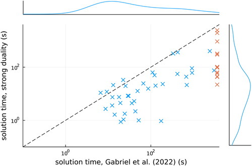
We compare the performance of the two single-level reformulations, the LCP-based reformulation from Gabriel, et al. (Citation2022) (Section 2.3) and our strong duality reformulation (Section 2.4) by solving 50 randomly generated problems with two producers, five energy sources, three nodes, and three representative days. This problem size was chosen as the base case because it seems to be large enough to make the problems challenging to solve, but small enough for them to be mostly solvable within a time limit of 1 h.

The results are presented in , and the main observation here is that the novel strong duality formulation is faster in most cases. In , markers below the diagonal (dashed line) correspond to such cases. In 13 instances, the formulation of Gabriel, et al. (Citation2022) did not find an optimal solution in an hour while our strong duality formulation did. One major issue with both models compared here is that usually the first feasible solutions are found at the end of the solution process, and most of the solution time is spent on improving the dual bound without finding any feasible solutions. Nevertheless, changing solver parameters to emphasise finding feasible solutions was not found to have a major impact on performance.

Figure 1. Solution times for the two formulations on 50 random instances with 2 producers, 5 energy sources, 3 nodes, and 3 representative days. If one of the methods failed to find a solution within 3600 s, an orange marker is used, and the marginal distributions on the right and top sides exclude unsolved instances.

As discussed in Section 2.5, the strong duality formulation results in fewer constraints than the reformulation in Gabriel, et al. (Citation2022). Recall that in our models, complementarity constraints are formulated as SOS1 constraints. The model sizes in the base case test problems are presented in , and out of the two, our strong duality model is smaller, except for having one more quadratic SOS1 constraint to represent the strong duality constraint Equation(11i)(11i) $0 \leq ϵ ⊥ - \sum_{i \in I} (z_{i}^{⊤} F_{i} z_{i} + e_{i 3} {(x)}^{⊤} z_{i} - a_{i 3} {(x)}^{⊤} p_{i}) \geq 0,$ (11i) . In our model, all non-complementarity quadratic constraints are inequality constraints, while in the LCP-based model, there is one quadratic equality constraint (the first one in Equation(6h)(6h) ${(q + N_{x} x)}^{⊤} (\tilde{z} - \bar{z}) = 0, (M + M^{⊤}) (\tilde{z} - \bar{z}) = 0,$ (6h) ).

Table 1. Model sizes for the two reformulations.

Download CSV Display Table

Next, we analyse how problem size affects solution times by varying either the number of producers, energy sources, nodes, and representative days from the base case, one parameter at a time. The results are presented in . The medium-sized cases in each subfigure are similar to each other, which is expected as the problem sizes are the same. Varying the number of producers or energy sources seems to have only a small effect on the solution times while changing the number of nodes has a far stronger effect. The effect of the number of representative days is stronger than that of the number of producers and energy sources but seems to be weaker than that of the number of nodes.

Figure 2. Cumulative distribution functions of solution times for the two formulations with 1–3 producers, 4–6 energy sources, and 2–4 nodes and representative days. For each problem size, 50 instances are generated and solved.

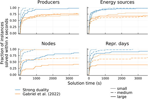
We can also see that the number of problems that were not solved to optimality within the time limit is affected by the number of nodes and representative days, but not by the number of firms or energy sources. Additionally, the novel strong duality model finds an optimal solution more frequently than the previous formulation. As predicted in Section 2.4, the larger number of complementarity constraints in the LCP formulation () proves to be computationally challenging, and the smaller strong duality model is solved faster.

4.2. Case study: a five-node Nordic energy system

The case study in Belyak et al. (Citation2023) considers five nodes, representing Finland, Sweden, Norway, Denmark, and the combined Baltic countries (Estonia, Latvia, and Lithuania). There are five producers, each owning production capacity in one of the five nodes. Nine different energy sources are available, consisting of five conventional sources: nuclear, coal, gas (closed- and open-cycle) and biomass, and four renewable sources: solar, hydro, onshore, and offshore wind. Additionally, we consider three representative days of renewable generation availability factors and demand curves. Recall that in our model, the top-level regulator makes their decisions independent of the day considered, that is, the carbon tax and minimum renewable share are constant across different representative days. These representative days are obtained in Belyak et al. (Citation2023) by performing hierarchical clustering on demand, price, and renewable availability data.

Day 1 is a winter day with higher demand, low solar availability, and medium wind availability. Days 2 and 3 have a lower demand with day 2 representing a windy day with medium solar availability, and day 3 representing a sunny day with low wind availability. The details of the hierarchical clustering process can be found in Belyak et al. (Citation2023).

In , the production portfolio (a weighted average over the representative days) is presented for a model with no carbon tax (i.e., the regulator heavily prefers maximising production over minimising emissions) and a carbon tax of 23 €/ton (enough to remove nearly all emissions). Compared to the baseline with no carbon tax, this 23 €/ton tax decreases the total production by 2.8%. In this example, these carbon tax values are achieved by setting the weight parameter r in the top-level objective Equation(12a)(12a) $max_{x, ρ, y, z} \sum_{d \in D} P_{d} \sum_{i \in I, j \in J, k \in K} (r - (1 - r) η_{ijk}) z_{ijkd}$ (12a) to 0.8 and 0.4, respectively.

Figure 3. Weighted average electricity production portfolio over the five nodes and three representative days.

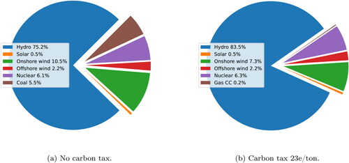
Because of the substantial hydropower production capacity in the Nordic system, particularly in Norway and Sweden (IRENA, Citation2023), the renewable share of production is large even without a carbon tax. A part of the increase in hydropower usage when the carbon tax is introduced comes from decreasing onshore wind production. This is a consequence of the simplified nature of the model and data, as the operational costs for both hydropower and onshore wind power are zero, resulting in multiple optima and indifference for the producers to use one or the other, as long as the production capacity of neither is exceeded. This artefact of the model could be easily removed by, e.g., setting the operational cost of either energy source to a small positive number instead of zero, causing the producers to prefer the cheaper source. However, this would imply an artificial preference for one source over the other. The only significant source of emissions is coal, and introducing a carbon tax of 23€/ton removes all coal from the portfolio, bringing in a small amount of closed-cycle gas power instead. The closed-cycle gas production occurs in the Baltics for day 1, and to understand this emergence of gas better, we must examine the transmission network in .

Figure 4. Transmission grid usage with different carbon taxes and representative days. The size of an arrow is proportional to the flow on the line and the colour of an arrow represents congestion: black arrows correspond to lines operating at their limit. The nodes are FI = Finland, SE = Sweden, NO = Norway, DK = Denmark, BA = Baltic countries.

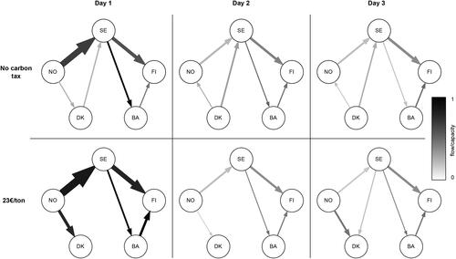
The first representative day has the highest network usage with large amounts of electricity transmitted from Norway to Finland through Sweden. With the carbon tax, the importance of transmission is further highlighted as the hydropower capacity in Norway is used for lowering overall prices under high demand and low production from both solar power and high-emission sources. The differences between representative days 2 and 3 are more subtle, but we can see, e.g., the reliance on wind power in Denmark: in the low-wind day 3, the carbon tax results in Denmark importing a significant amount of electricity from Norway, compared to the high-wind day 2. On the first day with a carbon tax of 23 €/ton, both lines connecting the Baltic countries to the rest of the system are at their capacity, explaining why the Baltic countries start using gas power after a carbon tax is introduced. This illustrates the complex interplay between the three levels that is captured by our model.

5. Conclusions

In this article, we propose a novel formulation for trilevel optimisation problems focusing on energy systems planning with environmental considerations. Additionally, we characterise the notion of weak and strong trilevel structures and compare the computational performance of the novel strong duality-based reformulation in this article and the LCP-based reformulation in Gabriel, et al. (Citation2022).

The computational results are encouraging, as we are able to solve the case study to optimality within a few minutes despite the fact that both single-level reformulations considered are non-convex problems. However, we note that preliminary experiments with seemingly small extensions to the model, such as adding ramping constraints (limiting the change in production between consecutive periods) to the producer problem made the problem computationally intractable. The small size of the case study is indicative of the very challenging (non-convex) nature of these problems, and the authors note that the reformulations and solution methods in this article should be viewed as one of the first steps towards an efficient solution framework for trilevel problems.

For the results in this article, an off-the-shelf solver is used, which is useful to ensure a low barrier-to-entry for using the developed formulation. However, we believe that the computational performance can be increased considerably using specialised solution methods like column-and-constraint generation (Dvorkin et al., Citation2018). Notably, ideas such as bilevel branch-and-bound (Fischetti et al., Citation2018) and convex hull reformulations of the middle-level feasible region (Santana and Dey, Citation2020) may be explored in the context of the problems presented in this article. In addition, the model could also be extended to consider transmission and/or production capacity expansion over multiple time periods, especially if computationally more efficient reformulations and solution methods are developed.

Despite the outstanding computational challenges, we show that the novel reformulation improves computational performance compared to the previous formulation (Gabriel, et al., Citation2022), and we show that the framework can be applied to a setting representing the Nordic electricity market, and results on the effect of carbon tax can be obtained. A limitation of the formulation approach presented in this article and that originally proposed by Gabriel, et al. (Citation2022) is that they require a weak trilevel structure. In practice, relevant problems may instead have a strong trilevel structure, precluding the use of these reformulations. Thus, further research is needed on developing (heuristic) solution methods for problems with a strong trilevel structure.

Disclosure statement

No potential conflict of interest was reported by the author(s).

Additional information

Funding

The calculations presented in this paper were performed using computer resources within the Aalto University School of Science “Science-IT” project. Fabricio Oliveira and Olli Herrala were supported by the Research Council of Finland (decision numbers 348094 and 332180). Steven A. Gabriel was supported by the National Science Foundation (NSF) Award #2113891, Civil Infrastructure Systems. Tommi Ekholm was supported by the Research Council of Finland (decision number 341311).

Notes

1 For completeness, the steps for obtaining the dual Equation(8)(8a) $max_{p_{i}, z_{i}} - \frac{1}{2} z_{i}^{⊤} F_{i} z_{i} + a_{i 3} {(x)}^{⊤} p_{i}$ (8a) from the primal problem Equation(7)(7a) $(P_{3 i} (x)) : min_{z_{i}} \frac{1}{2} z_{i}^{⊤} F_{i} z_{i} + e_{i 3} {(x)}^{⊤} z_{i}$ (7a) are presented in Appendix B.

2 For problems with only affine constraints, such as Equation(7)(7a) $(P_{3 i} (x)) : min_{z_{i}} \frac{1}{2} z_{i}^{⊤} F_{i} z_{i} + e_{i 3} {(x)}^{⊤} z_{i}$ (7a) , the Abadie constraint qualification is always satisfied (Bazaraa et al., Citation2013).

References

Bard, J. F. (1983). An algorithm for solving the general bilevel programming problem. Mathematics of Operations Research, 8(2), 260–272. https://doi.org/10.1287/moor.8.2.260
Web of Science ®Google Scholar
Bard, J. F. (1991). Some properties of the bilevel programming problem. Journal of Optimization Theory and Applications, 68(2), 371–378. https://doi.org/10.1007/BF00941574
Web of Science ®Google Scholar
Bard, J. F., & Moore, J. T. (1990). A branch and bound algorithm for the bilevel programming problem. SIAM Journal on Scientific and Statistical Computing, 11(2), 281–292. https://doi.org/10.1137/0911017
Web of Science ®Google Scholar
Baringo, L., & Conejo, A. J. (2012). Transmission and wind power investment. IEEE Transactions on Power Systems, 27(2), 885–893. https://doi.org/10.1109/TPWRS.2011.2170441
Web of Science ®Google Scholar
Bazaraa, M. S., Sherali, H. D., & Shetty, C. M. (2013). Nonlinear programming: Theory and algorithms. John Wiley & Sons.
Google Scholar
Beale, E. M. L., & Tomlin, J. A. (1970). Special facilities in a general mathematical programming system for non-convex problems using ordered sets of variables. Operational Research, 69(99), 447–454.
Google Scholar
Belyak, N., Gabriel, S. A., Khabarov, N., & Oliveira, F. (2023). Optimal transmission expansion planning in the context of renewable energy integration policies. https://doi.org/10.1016/j.jclepro.2024.141955
Google Scholar
Bezanson, J., Edelman, A., Karpinski, S., & Shah, V. B. (2017). Julia: A fresh approach to numerical computing. SIAM Review, 59(1), 65–98. https://doi.org/10.1137/141000671
Web of Science ®Google Scholar
Burr Metzler, C. (2000). Complementarity models of competitive oligopolistic electric power generation markets. [Doctoral dissertation, The Johns Hopkins University]. https://cats.informa.com/PTS/login.do https://www.proquest.com/openview/23325a82a09fd6418e0f13c0164e2dd6/1
Google Scholar
Camacho-Vallejo, J.-F., Corpus, C., & Villegas, J. G. (2023). Metaheuristics for bilevel optimization: A comprehensive review. Computers & Operations Research, 161, 106410. https://doi.org/10.1016/j.cor.2023.106410
Web of Science ®Google Scholar
Cottle, R. W., Pang, J.-S., & Stone, R. E. (2009). The linear complementarity problem. Society for Industrial and Applied Mathematics.
Google Scholar
Dempe, S., & Zemkoho, A. (Editors). (2020). Bilevel optimization. In: Panos M. Pardalos, My T. Thai (Series Editors), University of Florida. Springer optimization and its applications (Vol.161). Springer. Pages 3–26.
Google Scholar
Dorn, W. S. (1960). Duality in quadratic programming. Quarterly of Applied Mathematics, 18(2), 155–162. https://doi.org/10.1090/qam/112751
Google Scholar
Dunning, I., Huchette, J., & Lubin, M. (2017). JuMP: A modeling language for mathematical optimization. SIAM Review, 59(2), 295–320. https://doi.org/10.1137/15M1020575
Web of Science ®Google Scholar
Dvorkin, Y., Fernandez-Blanco, R., Wang, Y., Xu, B., Kirschen, D. S., Pandzic, H., Watson, J.-P., & Silva-Monroy, C. A. (2018). Co-planning of investments in transmission and merchant energy storage. IEEE Transactions on Power Systems, 33(1), 245–256. https://doi.org/10.1109/TPWRS.2017.2705187
Web of Science ®Google Scholar
Facchinei, F., & Kanzow, C. (2010). Generalized Nash equilibrium problems. Annals of Operations Research, 175(1), 177–211. https://doi.org/10.1007/s10479-009-0653-x
Web of Science ®Google Scholar
Fischetti, M., Ljubić, I., Monaci, M., & Sinnl, M. (2018). On the use of intersection cuts for bilevel optimization. Mathematical Programming, 172(1–2), 77–103. https://doi.org/10.1007/s10107-017-1189-5
Web of Science ®Google Scholar
Gabriel, S. A., Conejo, A. J., Fuller, J. D., Hobbs, B. F., & Ruiz, C. (2012). Complementarity modeling in energy markets. Springer Science & Business Media.
Google Scholar
Gabriel, S. A., Leal, M., & Schmidt, M. (2022). On linear bilevel optimization problems with complementarity-constrained lower levels. Journal of the Operational Research Society, 73(12), 2706–2716. https://doi.org/10.1080/01605682.2021.2015254
Web of Science ®Google Scholar
Gao, S., & Liu, N. (2021). Improving the resilience of port–hinterland container logistics transportation systems: A bi-level programming approach. Sustainability, 14(1), 180. https://doi.org/10.3390/su14010180
Web of Science ®Google Scholar
Gu, Y., Cai, X., Han, D., & Wang, D. Z. (2019). A tri-level optimization model for a private road competition problem with traffic equilibrium constraints. European Journal of Operational Research, 273(1), 190–197. https://doi.org/10.1016/j.ejor.2018.07.041
Web of Science ®Google Scholar
Gurobi Optimization, LLC. (2022). Gurobi Optimizer Reference Manual. https://www.gurobi.com
Google Scholar
Hájek, M., Zimmermannová, J., Helman, K., & Rozenský, L. (2019). Analysis of carbon tax efficiency in energy industries of selected EU countries. Energy Policy, 134, 110955. https://doi.org/10.1016/j.enpol.2019.110955
Web of Science ®Google Scholar
Hirth, L., Mühlenpfordt, J., & Bulkeley, M. (2018). The ENTSO-E transparency platform–A review of Europe’s most ambitious electricity data platform. Applied Energy, 225, 1054–1067. https://doi.org/10.1016/j.apenergy.2018.04.048
Web of Science ®Google Scholar
Hobbs, B. F. (2001). Linear complementarity models of Nash-Cournot competition in bilateral and POOLCO power markets. IEEE Transactions on Power Systems, 16(2), 194–202. https://doi.org/10.1109/59.918286
Web of Science ®Google Scholar
Huppmann, D., & Egerer, J. (2015). National-strategic investment in European power transmission capacity. European Journal of Operational Research, 247(1), 191–203. https://doi.org/10.1016/j.ejor.2015.05.056
Web of Science ®Google Scholar
Ilic, M., Galiana, F., & Fink, L. (1998). Power systems restructuring: Engineering and economics. Kluwer Academic Publishers.
Google Scholar
IRENA (2023). Renewable capacity statistics 2023. International Renewable Energy Agency.
Google Scholar
Jin, S., & Ryan, S. M. (2014). A tri-level model of centralized transmission and decentralized generation expansion planning for an electricity market—Part I. IEEE Transactions on Power Systems, 29(1), 132–141. https://doi.org/10.1109/TPWRS.2013.2280085
Google Scholar
Karush, W. (1939). Minima of functions of several variables with inequalities as side conditions [Master’s thesis, University of Chicago].
Google Scholar
Keles, D., Dehler-Holland, J., Densing, M., Panos, E., & Hack, F. (2020). Cross-border effects in interconnected electricity markets-an analysis of the Swiss electricity prices. Energy Economics, 90, 104802. https://doi.org/10.1016/j.eneco.2020.104802
Web of Science ®Google Scholar
Kieffer, E., Danoy, G., Brust, M. R., Bouvry, P., & Nagih, A. (2020). Tackling large-scale and combinatorial bi-level problems with a genetic programming hyper-heuristic. IEEE Transactions on Evolutionary Computation, 24(1), 44–56. https://doi.org/10.1109/TEVC.2019.2906581
Web of Science ®Google Scholar
Kleinert, T., Labbé, M., Ljubić, I., & Schmidt, M. (2021). A survey on mixed-integer programming techniques in bilevel optimization. EURO Journal on Computational Optimization, 9, 100007. https://doi.org/10.1016/j.ejco.2021.100007
Web of Science ®Google Scholar
Köppl, A., & Schratzenstaller, M. (2023). Carbon taxation: A review of the empirical literature. Journal of Economic Surveys, 37(4), 1353–1388. https://doi.org/10.1111/joes.12531
Web of Science ®Google Scholar
Kuhn, H. W., & Tucker, A. W. (1951). Nonlinear programming. Berkeley Symposium on Mathematical Statistics and Probability, 1951, 481–492.
Google Scholar
Leyffer, S., Menickelly, M., Munson, T., Vanaret, C., & Wild, S. M. (2020). A survey of nonlinear robust optimization. Information Systems and Operational Research, 58(2), 342–373. https://doi.org/10.1080/03155986.2020.1730676
Web of Science ®Google Scholar
Nahmmacher, P., Schmid, E., Knopf, B. (2014). Documentation of LIMES-EU - A long-term electricity system model for Europe. Retrieved February 22, 2024, from https://www.pik-potsdam.de/en/institute/departments/transformation-pathways/models/limes/DocumentationLIMESEU_2014.pdf
Google Scholar
Pineda, S., Bylling, H., & Morales, J. (2018). Efficiently solving linear bilevel programming problems using off-the-shelf optimization software. Optimization and Engineering, 19(1), 187–211. https://doi.org/10.1007/s11081-017-9369-y
Web of Science ®Google Scholar
Poncelet, K., Hoschle, H., Delarue, E., Virag, A., & Drhaeseleer, W. (2017). Selecting representative days for capturing the implications of integrating intermittent renewables in generation expansion planning problems. IEEE Transactions on Power Systems, 32(3), 1936–1948. https://doi.org/10.1109/TPWRS.2016.2596803
Web of Science ®Google Scholar
Ribó-Pérez, D., Van der Weijde, A. H., & Álvarez-Bel, C. (2019). Effects of self-generation in imperfectly competitive electricity markets: The case of Spain. Energy Policy, 133, 110920. https://doi.org/10.1016/j.enpol.2019.110920
Web of Science ®Google Scholar
Ruiz, C., Conejo, A. J., & Smeers, Y. (2012). Equilibria in an oligopolistic electricity pool with stepwise offer curves. IEEE Transactions on Power Systems, 27(2), 752–761. https://doi.org/10.1109/TPWRS.2011.2170439
Web of Science ®Google Scholar
Santana, A., & Dey, S. S. (2020). The convex hull of a quadratic constraint over a polytope. SIAM Journal on Optimization, 30(4), 2983–2997. https://doi.org/10.1137/19M1277333
Web of Science ®Google Scholar
Sauma, E. E., & Oren, S. S. (2007). Economic criteria for planning transmission investment in restructured electricity markets. IEEE Transactions on Power Systems, 22(4), 1394–1405. https://doi.org/10.1109/TPWRS.2007.907149
Web of Science ®Google Scholar
Siddiqui, S., & Gabriel, S. A. (2013). An SOS1-based approach for solving MPECs with a natural gas market application. Networks and Spatial Economics, 13(2), 205–227. https://doi.org/10.1007/s11067-012-9178-y
Web of Science ®Google Scholar
Sinha, A., Malo, P., & Deb, K. (2018). A review on bilevel optimization: From classical to evolutionary approaches and applications. IEEE Transactions on Evolutionary Computation, 22(2), 276–295. https://doi.org/10.1109/TEVC.2017.2712906
Web of Science ®Google Scholar
Slater, M. (1950). Lagrange multipliers revisited. Cowles Foundation Discussion Papers, 304.
Google Scholar
Still, G. (2002). Linear bilevel problems: Genericity results and an efficient method for computing local minima. Mathematical Methods of Operations Research, 55(3), 383–400. https://doi.org/10.1007/s001860200189
Web of Science ®Google Scholar
Ye, J. J., & Zhu, D. (1995). Optimality conditions for bilevel programming problems. Optimization, 33(1), 9–27. https://doi.org/10.1080/02331939508844060
Google Scholar
Young, D. (2020). US-REGEN model documentation. Retrieved February 22, 2024, from https://www.epri.com/research/products/3002016601
Google Scholar

Appendix A.

Reformulation of a bottom-level LCP with a positive semi-definite M

Cottle et al. (Citation2009) show that if the matrix M is positive semi-definite (PSD), all solutions to the LCP (A1) $0 \leq z ⊥ q + N_{x} x + N_{y} y + Mz \geq 0,$ (A1) can be obtained as the following polyhedral set: (A2) $\begin{matrix} {z \in R_{\geq 0}^{n_{z}} : q + N_{x} x + N_{y} y + Mz \geq 0, \\ {(q + N_{x} x + N_{y} y)}^{T} (z - \bar{z}) = 0, \\ (M + M^{T}) (z - \bar{z}) = 0}, \end{matrix}$ (A2) where $\bar{z}$ is a solution to the LCP.

Hence, the middle-level problem can be rewritten as (A3a) $mi n_{y, z \geq 0} d_{2}^{⊤} y + e_{2}^{⊤} z$ (A3a) (A3b) $s . t . A_{2} x + B_{2} y + C_{2} z \geq a_{2}$ (A3b) (A3c) $q + N_{x} x + N_{y} y + Mz \geq 0$ (A3c) (A3d) ${(q + N_{x} x + N_{y} y)}^{⊤} (z - \bar{z}) = 0$ (A3d) (A3e) $(M + M^{⊤}) (z - \bar{z}) = 0.$ (A3e)

We observe that Equation(A3d)(A3d) ${(q + N_{x} x + N_{y} y)}^{⊤} (z - \bar{z}) = 0$ (A3d) includes a bilinear term $y^{⊤} N_{y}^{⊤} z$ in an equality constraint. This is a non-convex constraint, precluding the direct use of KKT conditions for obtaining an optimal solution to Equation(A3)(A3a) $mi n_{y, z \geq 0} d_{2}^{⊤} y + e_{2}^{⊤} z$ (A3a) . However, for problems with a weak trilevel structure, N_y = 0 and these bilinear terms vanish. In the next theorem, we assume N_y = 0.

Theorem A.1.

Let M be a positive semi-definite matrix. Then, $(x^{*}, y^{*}, z^{*})$ is an optimal solution of Problem Equation(3)(3a) $(P_{1}) : mi n_{x, y, z} c_{1}^{⊤} x + d_{1}^{⊤} y + e_{1}^{⊤} z$ (3a) with middle level Equation(4)(4a) $(P_{2} (x)) : mi n_{y, z} d_{2}^{⊤} y + e_{2}^{⊤} z$ (4a) if and only if $(x^{*}, y^{*}, z^{*}, {\bar{z}}^{*})$ is an optimal solution of the problem(A4a) $mi n_{x, y, z, \bar{z}} c_{1}^{⊤} x + d_{1}^{⊤} y + e_{1}^{⊤} z$ (A4a) (A4b) $s . t . A_{1} x + B_{1} y + C_{1} z \geq a_{1}$ (A4b) (A4c) $\begin{matrix} \bar{z} \in \underset{z' \geq 0}{arg min} {z'^{⊤} (q + N_{x} x + Mz') : \\ q + N_{x} x + Mz' \geq 0 (β)}, \end{matrix}$ (A4c) (A4d) $\begin{matrix} y, z \in \underset{\hat{y}, \hat{z} \geq 0}{arg min} {d_{2}^{⊤} \hat{y} + e_{2}^{⊤} \hat{z} : \\ q + N_{x} x + M \hat{z} \geq 0 (δ) \\ {(q + N_{x} x)}^{⊤} (\hat{z} - \bar{z}) = 0 (ζ) \\ (M + M^{⊤}) (\hat{z} - \bar{z}) = 0 (η) \\ A_{2} x + B_{2} \hat{y} + C_{2} \hat{z} \geq a_{2} (γ)}, \\ such that {({\bar{z}}^{*})}^{⊤} (q + N_{x} x^{*} + M {\bar{z}}^{*}) = 0. \end{matrix}$ (A4d)

See Theorem 6 in Gabriel et al. (Citation2022) for a proof of this result as well as related theoretical aspects of the general form of the problem.

The two nested optimisation problems in Equation(A4)(A4a) $mi n_{x, y, z, \bar{z}} c_{1}^{⊤} x + d_{1}^{⊤} y + e_{1}^{⊤} z$ (A4a) are a convex QP Equation(A4c)(A4c) $\begin{matrix} \bar{z} \in \underset{z' \geq 0}{arg min} {z'^{⊤} (q + N_{x} x + Mz') : \\ q + N_{x} x + Mz' \geq 0 (β)}, \end{matrix}$ (A4c) and an LP Equation(A4d)(A4d) $\begin{matrix} y, z \in \underset{\hat{y}, \hat{z} \geq 0}{arg min} {d_{2}^{⊤} \hat{y} + e_{2}^{⊤} \hat{z} : \\ q + N_{x} x + M \hat{z} \geq 0 (δ) \\ {(q + N_{x} x)}^{⊤} (\hat{z} - \bar{z}) = 0 (ζ) \\ (M + M^{⊤}) (\hat{z} - \bar{z}) = 0 (η) \\ A_{2} x + B_{2} \hat{y} + C_{2} \hat{z} \geq a_{2} (γ)}, \\ such that {({\bar{z}}^{*})}^{⊤} (q + N_{x} x^{*} + M {\bar{z}}^{*}) = 0. \end{matrix}$ (A4d) . Hence, the KKT conditions of both problems are necessary and sufficient for optimality and the two inner problems can be replaced by their necessary and sufficient KKT conditions, leading to the single-level reformulation Equation(6)(6a) $min_{x, y, \tilde{z}, \bar{z}, β, γ, δ, ζ, η} c_{1}^{⊤} x + d_{1}^{⊤} y + e_{1}^{⊤} \tilde{z}$ (6a) .

Appendix B.

Formulating the dual of a QP with affine constraints

Given a quadratic program with affine constraints (B1a) $min_{z_{i}} \frac{1}{2} z_{i}^{⊤} F_{i} z_{i} + e_{i 3} {(x)}^{⊤} z_{i}$ (B1a) (B1b) $s . t . C_{i 3} z_{i} \geq a_{i 3} (x) (p_{i})$ (B1b) (B1c) $z_{i} \geq 0 (s_{i}),$ (B1c) where we assume F_i is a positive semi-definite (PSD) symmetric matrix, the Lagrangian of the problem is (B2) $L (z_{i}, s_{i}, p_{i}) = \frac{1}{2} z_{i}^{⊤} F_{i} z_{i} + e_{i 3} {(x)}^{⊤} z_{i} + p_{i}^{⊤} (a_{i 3} (x) - C_{i 3} z_{i}) - s_{i}^{⊤} z_{i},$ (B2) where p_i and s_i are non-negative Lagrange multipliers or dual variables. The first-order optimality condition is thus (B3) $\nabla_{z_{i}} L (z_{i}, s_{i}, p_{i}) = F_{i} z_{i} + e_{i 3} (x) - C_{i 3}^{⊤} p_{i} - s_{i} = 0$ (B3) and rearranging Equation(B2)(B2) $L (z_{i}, s_{i}, p_{i}) = \frac{1}{2} z_{i}^{⊤} F_{i} z_{i} + e_{i 3} {(x)}^{⊤} z_{i} + p_{i}^{⊤} (a_{i 3} (x) - C_{i 3} z_{i}) - s_{i}^{⊤} z_{i},$ (B2) gives us (B4) $\frac{1}{2} z_{i}^{⊤} F_{i} z_{i} - z_{i}^{⊤} C_{i 3}^{⊤} p_{i} + z_{i}^{⊤} e_{i 3} (x) - z_{i}^{⊤} s_{i} + a_{i 3} {(x)}^{⊤} p_{i},$ (B4) which, using the first-order condition $- F_{i} z_{i} = - C_{i 3}^{⊤} p_{i} + e_{i 3} (x) - s_{i},$ becomes (B5) $- \frac{1}{2} z_{i}^{⊤} F_{i} z_{i} + a_{i 3} {(x)}^{⊤} p_{i} .$ (B5)

Maximising EquationEq. (B5)(B5) $- \frac{1}{2} z_{i}^{⊤} F_{i} z_{i} + a_{i 3} {(x)}^{⊤} p_{i} .$ (B5) , subject to the first-order optimality condition for z_i and treating s_i as a slack variable and removing its explicit representation from the problem results in the Lagrangian dual formulation (B6a) $max_{p_{i}, z_{i}} - \frac{1}{2} z_{i}^{⊤} F_{i} z_{i} + a_{i 3} {(x)}^{⊤} p_{i}$ (B6a) (B6b) $s . t . C_{i 3}^{⊤} p_{i} - F_{i} z_{i} \leq e_{i 3} (x)$ (B6b) (B6c) $p_{i} \geq 0.$ (B6c)

Appendix C.

Further substitutions for the middle and bottom levels

The producer model can be further simplified using the substitution $s_{ikd} = \sum_{j \in J} z_{ijkd},$ removing the sales variables and the balance constraint Equation(17c)(17c) $\sum_{k \in K} s_{ikd} = \sum_{j \in J, k \in K} z_{ijkd} (θ_{id})$ (17c) . For a further reduction, the remaining equality constraints Equation(17d)(17d) $α_{kd} - β_{kd} (\sum_{i' \in I} s_{i' kd} + a_{ikd}) = p_{id}^{H} + w_{kd} \forall k \in K$ (17d) and Equation(17e)(17e) $\sum_{k \in K} a_{ikd} = 0$ (17e) can be used to solve for a and p^H.

We have the necessary and sufficient KKT conditions (C1) $α_{kd} - β_{kd} (\sum_{i' \in I} s_{i' kd} + a_{ikd}) = p_{id}^{H} + w_{kd} \forall k \in K$ (C1) (C2) $\sum_{k \in K} a_{ikd} = 0$ (C2) of the arbitrager’s problem, and with the substitution $\sum_{j \in J} z_{ijkd} = s_{ikd},$ we get (C4) $α_{kd} - β_{kd} (Z_{kd} + a_{ikd}) = p_{id}^{H} + w_{kd} \forall k \in K$ (C4) (C5) $\sum_{k \in K} a_{ikd} = 0,$ (C5) where $Z_{kd} = \sum_{i \in F, j \in J} z_{ijkd} .$ In matrix form, we get (C7) $[\begin{matrix} Q_{d} & 1 \\ 1^{⊤} & 0 \end{matrix}] [\begin{matrix} a_{id} \\ p_{id}^{H} \end{matrix}] = [\begin{matrix} α_{d} - Q Z_{d} - w_{d} \\ 0 \end{matrix}],$ (C7) where Q_d is a square diagonal matrix with the element on the kth row and column being β_kd and $1$ is a vector of ones. It can be shown that (C8) ${[\begin{matrix} Q_{d} & 1 \\ 1^{⊤} & 0 \end{matrix}]}^{- 1} = [\begin{matrix} L^{d} & h_{d} \\ h_{d}^{⊤} & {\hat{h}}_{d} \end{matrix}],$ (C8) where $\begin{matrix} {\hat{h}}_{d} = \frac{1}{\sum_{k \in K} β_{kd}^{- 1}} \\ h_{kd} = β_{kd}^{- 1} {\hat{h}}_{d} \\ L_{k, k}^{d} = {\hat{h}}_{d} β_{kd}^{- 1} \sum_{k' \in K ∖ k} β_{k′d}^{^{- 1}} \\ L_{k, k'}^{d} = - {\hat{h}}_{d} β_{kd}^{- 1} β_{k′d}^{^{- 1}}, k \neq k' . \end{matrix}$

This results in the solution (C9) $a_{ikd} = h_{kd} Z_{d} - Z_{kd} - \sum_{k' \in K} (α_{k' d} - w_{k' d}) L_{k, k'}^{d}$ (C9) (C10) $p_{id}^{H} = \sum_{k \in K} (α_{kd} - w_{kd}) h_{kd} - Z_{d} {\hat{h}}_{d},$ (C10) where $\begin{matrix} Z_{d} = \sum_{i \in I, j \in J, k \in K} z_{ijkd} \\ Z_{kd} = \sum_{i \in I, j \in J} z_{ijkd} . \end{matrix}$

It can be seen that the values of a_ikd and $P_{id}^{H}$ are the same for each firm $i \in I$ and we can drop the index i. Burr Metzler (Citation2000) shows that the arbitrage amounts correspond to the transmission values: a_kd = y_kd.

These substitutions result in the problem formulation (C11a) $max_{z_{id}} (\sum_{k \in K} (α_{kd} - w_{kd}) h_{kd} - Z_{d} {\hat{h}}_{d}) Z_{id} - \sum_{j \in J, k \in K} (γ_{ijk} - w_{kd}) z_{ijkd}$ (C11a) (C11b) $s . t . z_{ijkd} \leq z_{ijkd}^{max} (λ_{ijkd}) \forall j \in J, k \in K$ (C11b) (C11c) $z_{ijkd} \geq 0$ (C11c) and we can see that the substitutions do not change the concavity of the objective function: the quadratic term for producer $i \in I$ is ${\hat{h}}_{d} Z_{id}^{2} .$ Finally, the sales variables s_ikd are also eliminated from the market-clearing constraint, resulting in (C12) $h_{kd} Z_{d} - Z_{kd} + \sum_{k' \in K} (α_{k' d} - w_{k' d}) L_{kk'}^{d} = y_{kd} (w_{kd}) \forall k \in K .$ (C12)

The formulation Equation(C11)(C11a) $max_{z_{id}} (\sum_{k \in K} (α_{kd} - w_{kd}) h_{kd} - Z_{d} {\hat{h}}_{d}) Z_{id} - \sum_{j \in J, k \in K} (γ_{ijk} - w_{kd}) z_{ijkd}$ (C11a) can be converted into an LCP by using the KKT optimality conditions. The combined KKT conditions of Equation(C11)(C11a) $max_{z_{id}} (\sum_{k \in K} (α_{kd} - w_{kd}) h_{kd} - Z_{d} {\hat{h}}_{d}) Z_{id} - \sum_{j \in J, k \in K} (γ_{ijk} - w_{kd}) z_{ijkd}$ (C11a) for all producers $i \in I$ are (C13a) $0 \leq z_{d} ⊥ B_{d} z_{d} + λ_{d} + q_{d}^{z} \geq 0$ (C13a) (C13b) $0 \leq λ_{d} ⊥ - z_{d} + z_{d}^{max} \geq 0,$ (C13b) where $q_{ijkd}^{z} = - \sum_{k \in K} (α_{kd} - w_{kd}) h_{kd} + (γ_{ijk} - w_{kd})$ and B_d is a PSD matrix with $B_{d} (ijk, i' j' k') = {\begin{matrix} 2 {\hat{h}}_{d} & i = i' \\ {\hat{h}}_{d} & i \neq i', \end{matrix}$ making the bottom level an LCP with a PSD coefficient matrix $[\begin{matrix} B_{d} & I \\ - I & 0 \end{matrix}] .$ This makes the problem setting suitable for the method described in Section 2.3, but we will continue by presenting the strong duality approach to this problem.

C.1 Strong duality reformulation of the trilevel electricity market model

Using the primal–dual conversion rules for quadratic programs summarised in Dorn (Citation1960), the dual of the bottom-level problem Equation(C11)(C11a) $max_{z_{id}} (\sum_{k \in K} (α_{kd} - w_{kd}) h_{kd} - Z_{d} {\hat{h}}_{d}) Z_{id} - \sum_{j \in J, k \in K} (γ_{ijk} - w_{kd}) z_{ijkd}$ (C11a) can be stated as (C14a) $min_{λ_{ijkd}, z_{ijkd}} {\hat{h}}_{d} Z_{id}^{2} + \sum_{j \in J, k \in K} z_{ijkd}^{max} λ_{ijkd}$ (C14a) (C14b) $\begin{matrix} s . t . - λ_{ijkd} \leq \hat{h} d (Z_{d} + Z_{id}) - \sum_{k \in K} h_{kd} (α_{kd} - w_{kd}) \\ + (γ_{ijk} - w_{kd}) (z_{ijkd}) \forall j \in J, k \in K \end{matrix}$ (C14b) (C14c) $z_{ijkd}, λ_{ijkd} \geq 0.$ (C14c)

As described in Section 2.4, we impose a strong duality constraint stating that the objective value of the dual (minimisation) problem is less or equal to that of the primal (maximisation) problem, and combine constraints Equation(C11b)(C11b) $s . t . z_{ijkd} \leq z_{ijkd}^{max} (λ_{ijkd}) \forall j \in J, k \in K$ (C11b) –Equation(C11c)(C11c) $z_{ijkd} \geq 0$ (C11c) , Equation(C14b)(C14b) $\begin{matrix} s . t . - λ_{ijkd} \leq \hat{h} d (Z_{d} + Z_{id}) - \sum_{k \in K} h_{kd} (α_{kd} - w_{kd}) \\ + (γ_{ijk} - w_{kd}) (z_{ijkd}) \forall j \in J, k \in K \end{matrix}$ (C14b) –Equation(C14c)(C14c) $z_{ijkd}, λ_{ijkd} \geq 0.$ (C14c) and the strong duality constraint. A solution that satisfies these constraints must be optimal to Equation(C11)(C11a) $max_{z_{id}} (\sum_{k \in K} (α_{kd} - w_{kd}) h_{kd} - Z_{d} {\hat{h}}_{d}) Z_{id} - \sum_{j \in J, k \in K} (γ_{ijk} - w_{kd}) z_{ijkd}$ (C11a) and Equation(C14)(C14a) $min_{λ_{ijkd}, z_{ijkd}} {\hat{h}}_{d} Z_{id}^{2} + \sum_{j \in J, k \in K} z_{ijkd}^{max} λ_{ijkd}$ (C14a) . Notice that the inequality version of the strong duality constraint is convex (as opposed to an equality constraint between the primal and dual objective values), and the other constraints are affine.

Finally, we can write the primal and dual constraints and the strong duality constraint as (C15a) $z_{ijkd} \leq z_{ijkd}^{max} (λ'_{ijkd}) \forall i \in I, j \in J, k \in K$ (C15a) (C15b) $\begin{matrix} - λ_{ijkd} - {\hat{h}}_{d} (Z_{d} + Z_{id}) \leq - \sum_{k \in K} (α_{kd} - w_{kd}) h_{kd} \\ + (γ_{ijkd} - w_{kd}) (z'_{ijkd}) \forall i \in I, j \in J, k \in K \end{matrix}$ (C15b) (C15c) $\begin{matrix} \sum_{i \in I} ({\hat{h}}_{d} Z_{id}^{2} + {\hat{h}}_{d} Z_{d} Z_{id} + \sum_{j \in J, k \in K} z_{ijkd}^{max} λ_{ijkd} - (\sum_{k \in K} (α_{kd} - w_{kd}) h_{kd}) Z_{id} \\ + \sum_{j \in J, k \in K} (γ_{ijk} - w_{kd}) z_{ijkd}) \leq 0 (ϵ_{d}) \end{matrix}$ (C15c) (C15d) $z_{ijkd}, λ_{ijkd} \geq 0,$ (C15d) where the strong duality constraints for all producers $i \in I$ have been combined into a single constraint Equation(C15c)(C15c) $\begin{matrix} \sum_{i \in I} ({\hat{h}}_{d} Z_{id}^{2} + {\hat{h}}_{d} Z_{d} Z_{id} + \sum_{j \in J, k \in K} z_{ijkd}^{max} λ_{ijkd} - (\sum_{k \in K} (α_{kd} - w_{kd}) h_{kd}) Z_{id} \\ + \sum_{j \in J, k \in K} (γ_{ijk} - w_{kd}) z_{ijkd}) \leq 0 (ϵ_{d}) \end{matrix}$ (C15c) to reduce the number of constraints as suggested in Pineda et al. (Citation2018).

The KKT conditions of the ISO problem Equation(13)(13a) $max_{y_{kd}, z_{ijkd}} \sum_{k \in K} w_{kd} y_{kd}$ (13a) combined with the constraints Equation(C15)(C15a) $z_{ijkd} \leq z_{ijkd}^{max} (λ'_{ijkd}) \forall i \in I, j \in J, k \in K$ (C15a) and the market-clearing constraint Equation(C12)(C12) $h_{kd} Z_{d} - Z_{kd} + \sum_{k' \in K} (α_{k' d} - w_{k' d}) L_{kk'}^{d} = y_{kd} (w_{kd}) \forall k \in K .$ (C12) are (C16a) $\begin{matrix} 0 \leq z_{ijkd} ⊥ λ'_{ijkd} - {\hat{h}}_{d} (Z_{d} + Z_{id}) + (2 {\hat{h}}_{d} (Z_{d} + Z_{id}) - \sum_{k \in K} (α_{kd} - w_{kd}) h_{kd} + \\ (γ_{ijkd} - w_{kd})) ϵ_{d} - (I (j \in R) - ρ) ψ_{kd} \geq 0 \forall i \in I, j \in J, k \in K \end{matrix}$ (C16a) (C16b) $0 \leq λ_{ijkd} ⊥ - z'_{ijkd} + z_{ijkd}^{max} ϵ_{d} \geq 0 \forall i \in I, j \in J, k \in K$ (C16b) (C16c) $0 \leq z'_{ijkd} ⊥ λ_{ijkd} + {\hat{h}}_{d} (Z_{d} + Z_{id}) - \sum_{k \in K} (α_{kd} - w_{kd}) h_{kd} + (γ_{ijkd} - w_{kd}) \geq 0 \forall i \in I, j \in J, k \in K$ (C16c) (C16d) $0 \leq λ'_{ijkd} ⊥ z_{ijkd}^{max} - z_{ijkd} \geq 0 \forall i \in I, j \in J, k \in K$ (C16d) (C16e) $0 \leq ϕ_{ad}^{-} ⊥ T_{a}^{-} + \sum_{k \in K} {PTDF}_{ka} y_{kd} \geq 0 \forall a \in A$ (C16e) (C16f) $0 \leq ϕ_{ad}^{+} ⊥ T_{a}^{+} - \sum_{k \in K} {PTDF}_{ka} y_{kd} \geq 0 \forall a \in A$ (C16f) (C16g) $0 \leq ψ_{kd} ⊥ \sum_{i \in I, j \in R} z_{ijkd} - ρ \sum_{i \in I, j \in J} z_{ijkd} \geq 0 \forall k \in K$ (C16g) (C16h) $\begin{matrix} 0 \leq ϵ_{d} ⊥ - \sum_{i \in I} ({\hat{h}}_{d} Z_{id}^{2} + {\hat{h}}_{d} Z_{D} Z_{id} + \sum_{j \in J, k \in K} z_{ijkd}^{max} λ_{ijkd} - \\ (\sum_{k \in K} (α_{kd} - w_{kd}) h_{kd}) Z_{id} + \sum_{j \in J, k \in K} (γ_{ijk} - w_{kd}) z_{ijkd}) \geq 0 \end{matrix}$ (C16h) (C16i) $w_{kd} = \sum_{a \in A} {PTDF}_{ka} (ϕ_{ad}^{+} - ϕ_{ad}^{-}) \forall k \in K$ (C16i) (C16j) $y_{kd} = - Z_{kd} + h_{kd} Z_{d} + \sum_{k' \in K} L_{k, k'}^{d} (α_{k' d} - w_{k' d}) \forall k \in K .$ (C16j)

The indicator term $I (j \in R)$ is 1 if $j \in R,$ 0 otherwise, and the variables $z'_{ijkd}$ and $λ'_{ijkd}$ are the dual variables of the primal and dual constraints from the producer level for the system operator problem, and ϵ is the dual variable for the strong duality constraint.

A novel strong duality-based reformulation for trilevel infrastructure models in energy systems development

Abstract

1. Introduction