Record linkage in the Cape of Good Hope Panel^*

Abstract

In this article, we describe the record linkage procedure to create a panel from Cape Colony census returns, or opgaafrolle, for 1787–1828, a dataset of 42,354 household-level observations. Based on a subset of manually linked records, we first evaluate statistical models and deterministic algorithms to best identify and match households over time. By using household-level characteristics in the linking process and near-annual data, we are able to create high-quality links for 84% of the dataset. We compare basic analyses on the linked panel dataset to the original cross-sectional data, evaluate the feasibility of the strategy when linking to supplementary sources, and discuss the scalability of our approach to the full Cape panel.

Keywords:

• Census
• machine learning
• micro-data
• record linkage
• panel data
• South Africa

Introduction

Improvements in computing power and novel analytical techniques allow for the reconstruction of historical populations in a way that has brought historical demography into the realm of big data (Ruggles 2012, 2014). Mass digitization of historical sources, particularly those containing individual-level information is now commonplace, and not only in the developed world (Dong et al. 2015; Fourie 2016). However, to enable in-depth life-course analyses, individuals need to be identified and linked across multiple, often disparate historical records (Bloothooft et al. 2015). Introducing a degree of automation into this process increases efficiency, but raises questions of accuracy and potential bias (Feigenbaum 2016).

In this article, we describe the record linkage strategy used to link households in the opgaafrolle tax records from the Cape Colony. The opgaafrolle were annual tax censuses collected between 1663 and 1834 of all free households of the Colony; first by the Dutch East India Company (VOC) administration and, after 1795, by the British colonial administration. Household-level information includes the name and surname of household head and spouse, the number of children present in the household, the number of slaves (and, in some cases, indigenous Khoesan employed), and several agricultural inputs and outputs, including cattle, sheep, horses, grain sown, grain reaped, vines and wine produced. Our ultimate goal is to create an annual panel of the agricultural production of households for over a century.

To create this panel, we evaluate a number of statistical models and deterministic algorithms to link households over time. After establishing the best approach based on a subset of manually linked records, we describe how we use this model to create a panel from the opgaafrolle for the Graaff-Reinet territory from 1787 to 1828, a 35-year, 42,354-observation dataset. We pay specific attention to the role of the panel nature of our data and the usage of household-level characteristics in attaining high linkage rates. We also compare basic correlations in the linked panel dataset to the original cross-sectional data. Next, we assess the re-usability and flexibility of our approach by adapting it to link the newly created panel dataset to a dataset of genealogical records of South African families, an independent dataset containing a different set of potential linking variables from the same period. We end with a discussion of the scalability of this approach to the full Cape panel.

Literature

Substantial efforts have already been made to link historical records in a systematic manner. Ferrie (1996) was among the first to use automated record linkage on historical data. His procedure to link individuals from the 1850 to the 1860 US census was based on the comparison of phonetically encoded names, year of birth, and birthplaces. In the decades since, record linkage has become an important tool in economic and social history, and methodological contributions have continued to be made (e.g., Ruggles 2002; Hautaniemi, Anderton, and Swedlund 2000; Rosenwaike et al. 1998). See also the review in Ruggles, Fitch, and Roberts (2018).

It is worthwhile to discuss a number of recent contributions. Vick and Huynh (2011) analyze how name standardization affects record linkage on the USA and Norwegian censuses. Using manually created first-name dictionaries to preprocess their linking data, they find improvements in linkage. Wisselgren et al. (2014) use a combination of three techniques to link Swedish population registers: manually standardized names, constructing surnames from patronymic naming practices, and using household information to make additional links between household members once the primary links have been established. Using this procedure on the high-quality Swedish population registers gives them linkage rates of 70%. Antonie et al. (2014) discuss their record linkage approach for the Canadian censuses of 1871 and 1881. While they use household-level characteristics to manually create their training data, automatic linkage is done based on individual-level characteristics only. Using a blocking strategy and a support vector machine (SVM) classifier, they achieve a linkage rate of 24%, with the largest share of missing links due to the discarding of ambiguous links. More recently, Massey (2017) evaluates historical record linkage practices by comparing their performance to high-quality links based on social security numbers. She finds that the use of string distance measures and probabilistic matching increases linkage rates substantially, but that this comes at the cost of a greater number of incorrect links.

Two articles deal explicitly with group versus individual-level linking, which is highly relevant to our method. Goeken et al. (2011) give an overview of the record linkage strategy used to create the IPUMS project’s United States Linked Samples, 1850–1930. They describe their strategy of blocking on race, gender, birthplace, and age range, the use of a SVM classifier, and a weighting procedure to correct for variable linkage rates across subpopulations. Of particular interest for the present article is their approach to linking households and individuals. Because they do not want to create a bias towards people who remain in the same households from one census to the next, their primary linking is done on individuals, not households. Once the individuals are confirmed, other individuals are linked across censuses based on the fact that they are in the same household. While overall linkage rates are not reported, they achieve high reliability in the links (less than 2% false positives).

Fu et al. (2014) describe a group and individual-based record linkage technique for historical censuses. They note that historical record linkage is particularly problematic due to data quality. The main issue is that existing procedures tend to generate multiple links, that is, matches are created where there are actually none. They propose using household-level characteristics, which are more likely to be unique over time, to resolve ambiguous links. Below we arrive at a similar conclusion: using additional household information can greatly improve linkage rates. The difference, however, is that we use household characteristics as the basis for primary links rather than as a tool for disambiguation after an initial linkage has been made.

Above all, the broad scope in methods and application of historical record-linkage suggest that a thorough understanding of the context is critical for developing a successful matching strategy, which is why we turn next to South Africa’s opgaafrolle.

The Opgaafrolle

When Europeans first settled at the southern tip of Africa, arriving in Table Bay in April 1652, their purpose was clear: to supply ships passing the Cape of Good Hope on their way to India and back to Europe with the necessary fresh produce, fuel and water. However, the small settlement was simply not large enough to produce enough food for its own survival and the almost 6000 soldiers and sailors that would frequent the Cape every year. In 1657, then, nine Company servants were released to become vryburghers (free settlers) and settle along the Liesbeeck River to farm. It was the beginning of a colonial society.

To keep track of the fluctuating levels of production in the fledging colonial society, the Company instituted annual tax censuses. It is unclear when the first proclamation for the opneemrolle, the name given to the tax censuses before 1794, or opgaafrolle, as they have since become known, were made. The inventory of the opgaafrolle in the Cape Archives Repository states that the “earliest reference to the submission of a return of people and possessions is found in the journal of 12 October 1672” (Potgieter and Visagie 1974).

Nevertheless, the household census of production became an annual event at the Cape soon after the establishment of a free settler society. The early censuses recorded only key household and production figures. Demographic information included the number of men, women, sons, daughters, European laborers, and slaves. Production information included the number of horses, cattle, and sheep owned, the number of vines planted and wine produced, as well as the volume of grains (wheat, barley, rye, and oats) sown and reaped. In addition, the number of flintlocks, pistols, and swords were also captured. Later censuses, particularly those after 1800, sporadically included additional production information, like the volume of brandy produced. Other assets, like wagons and carts, also appeared. Sometimes information on recapitulation totals, mortality rates, church contributions, and taxes paid are also included. In certain cases, the head of the household signed his or her name next to the record. It is these records the Cape of Good Hope Panel project is in the process of transcribing.

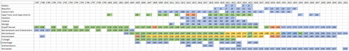
The original census returns pose many transcription challenges. There are often two returns for each year, a “concept return” and a “final return”. There are numerous examples where the two returns do not correspond perfectly; in one of them, or both, sub-districts are amiss. We follow the general rule of transcribing the “final return,” where possible. There are also several returns missing. Figure 1 shows all the census returns that are available in the Cape Town Archives Repository between 1787 and 1842, as indicated in the inventory. The inventory also provides a short description of each return. It frequently states that some returns, or parts thereof, are missing or unreadable. Although ordered chronologically, parts of some censuses appear in other districts or years. Other information, like lists of Khoesan inhabitants, cattle lists and even a poem written about census collection, are also included.

Figure 1. The series of opgaafrolle, 1787–1842, by district. Fully transcribed censuses in green, partially transcribed ones in yellow, illegible ones in red and the un-transcribed census returns in blue.

It is also useful to note what these census returns do not include. While the names of the husband and, usually, the wife are included, childrens’ names are not. Except for the name of the district and sometimes the name of the subdistrict, there is no information about the location of the household. Farm names are not included, for example. Occasionally, the names of the household heads are listed alphabetically but are most often ordered randomly. It may be that the order is an indication of proximity: names were recorded in the sequence that the surveyor traveled through the countryside, visiting homesteads. Most importantly for economic analysis, no information about the value of land, the size of farms or homesteads or other forms of wealth (except slaves, productive assets, and wagons and carts) are included.

Between January 2015 and April 2017, 100 census returns were transcribed in full, and the names for an additional 29 have been transcribed (Figure 1). The focus was initially on those records which also included numbers for Khoesan employed on settler farms. Such information was limited to the Graaff-Reinet and Tulbagh districts, the two frontier districts at the end of the eighteenth century on the eastern and northern borders of the 8 Colony, respectively. The third district to be transcribed was the Cape district, the returns for which differ substantially from those of the outlying regions. The Cape district returns are captured at the individual level rather than at the household level. We choose to focus here on the Graaff-Reinet district, the most complete and longest series transcribed at present.

The Cape of Good Hope Panel project aims to transcribe more than five times the number of censuses and link them, for the first time, across time. Below we describe the record linkage strategy we have developed to combine the opgaafrolle into what will become the world’s longest household-level panel dataset.

Record Linkage

Our record linkage process consists of the following steps. After basic data cleaning, candidates for comparison were created (blocking). Actual comparisons and linkage decisions were then made using a classifier which was trained on a manually linked subset of the data. The results of these comparisons were then used to create links between the censuses. Each of these steps is explained in more detail below.¹

The first step was to clean the data. All names were converted to the same case, encoding issues were fixed, nonletter characters were removed, and all characters were converted to ASCII. This latter step transliterated a few accented characters.² Initials were created from the first names.

Blocking—selecting candidates for more in-depth comparison—was the next step. This was necessary to prevent having to do computationally intensive full comparisons for all combinations of records (Christen 2012). We used the Jaro–Winkler string distance (with the penalty for mismatches in the first four characters set to 0.1) between men’s surnames as our blocking variable (Loo 2014). We selected as candidates all pairs of households whose length-normalized male surname string distance was less than 0.15.

This blocking strategy was found to be somewhat inefficient as the surname string distance still had to be calculated between all records. While calculating one string distance is still preferable over computing all string distances used in the in-depth comparison, it is still a computationally intensive step. A blocking strategy based on indexing would therefore be preferable, using for example ages, or soundex-encoded surnames. The opgaafrolle, however, do not report ages, and the diversity of origin of the settler population – including Dutch, French, English, and German origins—means that language-specific phonetic encodings are likely to be unreliable (Christen 2012). We do use phonetic string distances in the more detailed comparisons below because phonetically similar spelling variations can be important (for instance exchanging the letters C and K). At that detailed stage of the matching procedure, the use of soundex for the South African population is not problematic because uninformative variables do not end up contributing greatly to the predictions. However, selecting the candidates based on a potentially uninformative variable carries a high risk.

Since we only compare the observations from one year in one district (usually between 1,000 and 1,500 observations) to all the others in the district (the remainder of the 42,354 observations), the computational inefficiency of our procedure does not yet lead to problems. Future expansions of the procedure will, however, probably require an improved blocking strategy. Scalability issues are further discussed below.

Next, we use machine learning techniques to predict whether two candidate records belong to the same household. To do this, we began by manually creating a training dataset of 454 links based on 608 records from Graaff-Reinet in 1828 and 674 records from 1826. When manually matching individuals the following steps were followed: Names were arranged alphabetically in the two censuses. A large number of straightforward matches could be made on the basis of male first-names and surnames alone, as unique male first-names and surnames often existed across several years. The fact that 80% of males in our manually matched sample had more than one first name, also aided the matching process. Note that minor spelling variations between names were permitted – e.g. the surname “Ackerman” could be either “Akkerman” or “Ackermann” – but given the same unique first names, a true match was assigned. Knowledge about the idiosyncrasies of the Dutch/Afrikaans naming traditions proved particularly useful, for example, that “Johan” and “Jan” are both common short forms of the first name “Johannes”.

In some cases, however, owing to the tradition of naming oldest sons after their fathers or paternal grandfathers, certain first names, their ordering, and surnames repeated within a given census year, a match could not be made. This necessitated the consideration of the wife’s name and surname. Although we did not count how many names could be matched by simply using this procedure, we estimate that at least 70% of all pairs were successfully matched using only these four variables (names and surnames of husbands and wives). Where there was no wife present and two similar names appeared in the same year, manual matching became much more difficult, and subjective. Here, we erred on the side of caution; if two names could not be distinguished, we did not attempt a match. Sometimes, though, additional information, like “junior” or “widow”, would enable disambiguation between identical names. Sometimes a name was unique within a specific district, which allowed us to match the individual (assuming no migration). Occasionally, we also considered the number of children in the household or assets owned, although here, too, we erred on the side of caution. Quite frequently, while the husband’s name and surname might have been similar across years, the wife’s name would be somewhat different: for example, “Maria Magdelena” might become “Maria Elizabeth”. We then assumed that these were errors in the transcription process, or genuine errors in the original. There were also several cases where it was clear that the wife had died, and that the husband had remarried.

Almost 75% of names in the 1828 census could be manually linked to 1826. A retention rate of 75% is surprisingly high in this context given that this was a turbulent period on the Cape frontier, characterized by frequent skirmishes between the settlers, the indigenous Khoesan and amaXhosa, and the settlers’ semi-nomadic lifestyle with poor access to basic services. New migrants constantly entered and exited the district in search of land, or better economic opportunities. As far as we could establish from casual observation, the unmatched consisted of largely two groups: (i) Where a unique name and surname combination only existed in one year (this was the most likely reason for non-matches), and (ii) where two similar names existed in one year matched by similar names in another year but with no additional information, like wives’ names, to separate the two.

Using the blocking strategy described above, candidates were created for linkage from these 608/674 records to end up at a final training data set with 7,585 possible comparisons (candidate links) containing 454 true links. To train the models and assess their performance, we split this dataset in half. Having a separate test, dataset is important to check for overfitting (the tendency to fit the model to the training data’s idiosyncrasies rather than general features that will also hold for the rest of the data), a common issue with machine learning algorithms.

Table 2 presents the variables or features of the data that were used in the models. Some of these are commonly used in historical record linkage (Feigenbaum 2016; Goeken et al. 2011), while others are more specific to the opgaafrolle. We include string distances between the first names and surnames of the husbands and wives from one year to the next. The old and young indicator variables are also included.³ The nrdist variable is included to capture information about the order of the households in the returns.⁴ The wife-presence variables are important to include because the absence of the wife makes it far harder to identify a link.⁵ The string distances between the name of the husband and wife are meant to capture changes in recording the wife’s maiden name or her husband’s surname. Finally, the frequency of each surname was also included as a predictor variable, as common surnames are likely to be less predictive of linkages compared to rarer surnames.⁶

Table 2. Description of variables used in the record comparisons.

Variable	Explanation
namefreq_from/to	Frequency of name and similar variants in full opgaafrolle dataset
mlastdist	Jaro-Winkler string distance between husbands’ last names.
mfirstdist	Jaro-Winkler string distance between husbands’ first names.
minidist	Jaro-Winkler string distance between husbands’ initials.
wlastdist	Jaro-Winkler string distance between wives’ last names.
wfirstdist	Jaro-Winkler string distance between husbands’ first names.
winidist	Jaro-Winkler string distance between husbands’ initials.
mlastsdx	Soundex string distance between husbands’ last names.
mfirstsdx	Soundex string distance between husbands’ first names.
wlastsdx	Soundex string distance between wives’ last names.
wfirstsdx	Soundex string distance between wives’ first names.
nrdist	Difference between position in year’s opgaafrol.
bothyoung	Both individuals are identified as young.
bothold	Both individuals are identified as old.
dchildren	Difference in number of children present in households
spousenamedist_from/to	Jaro-Winkler string distance between husband and spouse surname
wife_present_from/to	Wife present in the “from” or “to” record
wifeinboth	Wife present in both records.
bothwineprod	Both records are indicated as wine producers (they have
mtchs	Number of candidates for this record.

We experimented with a number of models including support vector machines and neural networks, but focus here on two: logistic regression and the random forest classifier (Breiman 2001; Liaw and Wiener 2002). Logistic regression is included as a high-performing, yet easy-to-interpret classifier (Feigenbaum 2016). The random forest classifier is discussed because it is the best performing model of the ones we have tested.⁷

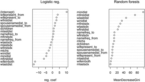
Figure 2 presents the regression coefficients for the logistic regression and the importance of variables in the random forest model. The models agree on a number of features. The string distance between the male first names, the initials, and the female last names are important in both models. The low importance of the string distance between male surnames in both models can be explained by the fact that they have already been used to select candidates (blocking). Thus, the male surnames within each block will be similar and contain little further information for prediction of matches within the block.

Figure 2. Regression coefficients for logistic regression (left panel) and variable importance plot for random forest model (right panel).

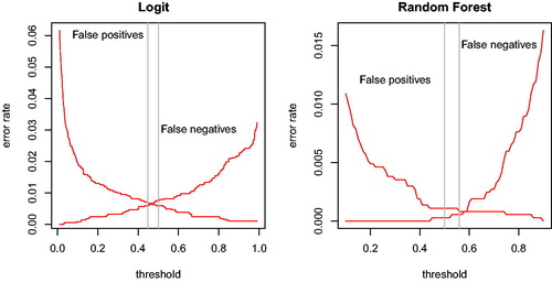
Most important for our purposes is the predictive performance of the models. Since both models give estimates of the probability that a link is true, a threshold at which we declare a link must first be determined. This is done by minimizing the error rate, based on combined number of false positives (where the model predicts a link in the test data that was not present in the training data) and false negatives (where the model incorrectly fails to predict a link in the test data that was present in the training data) as a share of the total number of observations (James et al. 2013).

Figure 3 shows that the false positive- and false-negative error rates are minimized below the conventional threshold of 0.5 in the case of logistic regression and at 0.56 in case of the random forest model. As we explain below, we are more concerned about creating false links that we are about missing true links. In the comparisons below, we thus stick to a 0.56 threshold for the random forest model. In the case of the logit model, we use a more conservative threshold of 0.5, thus lowering its false positive rate compared to the error rate-minimizing threshold. We include the predicted probability (or in the case of the random forest model, “votes”) of a true link in the data, so future users of the opgaafrolle database can increase the required confidence level and exclude less certain links. Note, however, that the number of false negatives increases sharply when we raise the threshold in the random forest model above 0.7, meaning one would miss a large number of true links.

Figure 3. Errors as share of total candidates in the training data as a function of the threshold for logistic regression (left panel) and for random forest (right panel) model. Vertical reference lines at error rate minimizing-vote share and 0.5.

The predictive performance of the two models is further investigated using the confusion matrices in Tables 3 and 4. These matrices show the true positives (where the model correctly predicts a link that was present in the training and test data), true negatives (where the model correctly predicts that a link was not present in the training and test data), false positives, and false negatives for the training and the test data. Because there are many candidates that are not actual links relative to the number of actual links, true negative rates are typically very high in record linkage and not informative about the quality of the matches (Christen 2012). We therefore focus on recall (the true positives as a share of the sum of true positives and false negatives, also known as the true positive rate) and the precision (the true positives as a share of the sum of the true positives and false positives).

Table 3. Confusion matrix for logit models.

		Predicted
		Train		Test
		False	True	False	True
Actual	0	3432	22	3558	20
	1	28	201	23	189

Table 4. Confusion matrix for random forests model.

		Predicted
		Train		Test
		False	True	False	True
Actual	0	3451	3	3566	12
	1	2	227	30	182

Both models have high recall. In case of the logit model, it is 88% on the training data and 89% on the test data (Table 3). The random forest model (Table 4) performs well on the training data (99.6% sensitivity), though its performance is lower than the logit model on the test data 86%), a sign of overfitting. Overall, our models perform well compared to other historical record linkage efforts, a point which we explain below.

Of the two main classifiers tested here, we prefer the random forest model for our linkage procedure. While both classifiers have similar sensitivity on the test data, the main reason for preferring the random forest model is that it has fewer false positives. Its precision on the test data is 94% compared to 90% in the logit model.⁸ Including false links is arguably worse than missing true links, since missing observations, while an issue, is a well-researched issue; consider, for instance, the literature on missing data, selection bias, and survey weighting (Little and Rubin 1987; Heckman 1979; Solon, Haider, and Wooldridge 2015; Antonie et al. 2014). On the other hand, there are no satisfying methods to deal with incorrectly matched observations (a similar point in Antonie et al. 2014). Another reason for preferring the random forest classifier is that the decision trees on which it is based are well suited to find any non-linearities and interactions that might exist in the data (Hastie, Tibshirani, and Friedman 2009, 587), which is relevant for record linkage.⁹

While we prefer the random forest classifier, it should be noted that logistic regression performs well here (see also Feigenbaum 2016), and could be preferable if interpretability of the classifier is important.

A manually weighted combination of string distances performed far worse than all models we tested. To create a set of weights that reflected what we deemed to be important in the linking procedure, we drew from our experience of manually matching the training data.¹⁰ We identified only 122 out of 229 true matches (53%) in the training data correctly. The false-positive and false-negative rate for this procedure were 7% and 47%, respectively.¹¹ Clearly, even relatively straightforward classifiers are superior in the case of the opgaafrolle data, probably because classic record linkage variables like age and place of birth are missing.

It is useful to investigate the false positives created by the random forest classifier in greater detail to understand in which cases our procedure fails. The preferred model creates 12 false positives in the test data (see appendix, section B.2). Of these, 6 lack information on the wife in both records. Based on only the husband’s name, all could be true links omitted in the creation of the training data, but were omitted because the link was ambiguous. The remaining six observations for which information about the wife is available are likely correct, but were not recognized as true links in the construction of the training data. In short, many of the false positives could be actual links in the training data.

The random forest model is not dependent on including all of the variables in Table 2. In appendix C, Tables A3 and A4 show that the area under the curve (AUC), a measure of the rate of true positives to the rate of false positives, remains close to the preferred model’s AUC of 0.94.¹²

Panel Linkage

We declare as links those candidates that get the highest score for their block, provided the score is above 0.56. To deal with the possibility of multiple links we rely on their absence in the training data, where ambiguous matches were explicitly not linked (see above). Our models include a number of variables to capture this aspect of the training data. Of these, the presence of a wife is important as the names of husband and wife often suffice to uniquely identify individuals in the Graaff-Reinet district. Our low false-positive rate indicates this method can be successful.

Since we are building a panel, we would expect to find one household in multiple years. This means the application of the model outlined above as well as the construction of the panel out of the suggested links require us to deal with a number of further issues.

Our approach has been to apply our linkage from each year to all earlier years (e.g., 1828 to 1826, 1825, …; 1826 to 1825, 1824, …, and so forth). We use this backwards procedure to exploit the fact that information is typically better for the more recent records. Once we move to the next base year for comparing, it is unnecessary to include the previous base year in the comparison. The string distance relations we use are symmetric, so if two years have been compared in one direction they do not need to be compared again. This allows us to economize on the number of comparisons we need to make. Working from one base year has the additional advantage of keeping the string distance matrix that serves as the basis for creating candidates small.

Working in a panel setting also creates the possibility of creating incomplete series of links (where, for example, observations 1 and 3, and 2 and 3 are matched, but observations 1 and 2 are not). In dealing with this issue, we have been permissive and have used the linkage information from various base-years to connect disjointed series. The main reason for doing this is that finding that a household is linked between certain census-years means this household should probably be present in intermediate years as well, but has been missed as a result of a transcription error, or simply excluded from the original census.

Finally, it is worth mentioning that the panel structure of the data could also be used to assist the linkage process. If, for example, we find an individual in 1828, 1826, and 1824, our expectation of finding him in 1825 is higher and this information should feed into the linkage procedure. We have not been able to implement this here, but suggest this as a fruitful avenue to pursue when linking panel data.

Dataset Evaluation

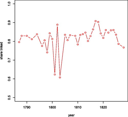
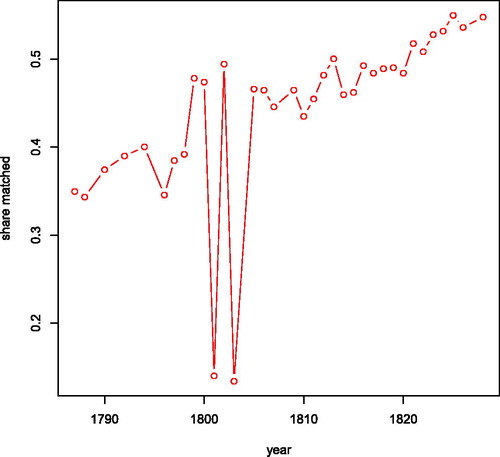
We now turn to the evaluation of the linked dataset. While success on the test data is the only certain assessment of the linkage procedure, manual inspection of the resulting series is also useful. This has so far not revealed obviously incorrect linkages. On average, the share of households in any other year being linked to any other year is over 80% (Figure 4). Usually, the figure is somewhat higher than that, but linking individuals to and from 1801 to 1803 proved more difficult because the opgaafrolle in those years rarely if ever contain information on wives. In these years, linkage drops to 60% of the households and many of our series end in one of these two years.

Figure 4. Share of households linked by year.

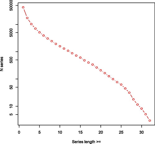
The longest series created are 32 observations long (figure 5). There are 3 of these series in the data, making for 96 observations in total. A shorter minimum length of linkages yields more observations: a minimum series length of 23 yields some 100 series. A lower threshold of a minimum series length of 8 yields over 2,000 series, covering almost 20,000 observations. With the Graaff-Reinet opgaafrolle for 1787–1828 containing 42,354 observations, this means that almost half of the observations are contained in these moderately long series. If series of at least three years are sufficient for an intended analysis, over two-thirds of the dataset (more than 10,000 series and over 30,000 observations) would be covered.

Figure 5. Cumulative links in opgaafrolle panel by series length. Number of series plotted on a (natural) logarithmic axis.

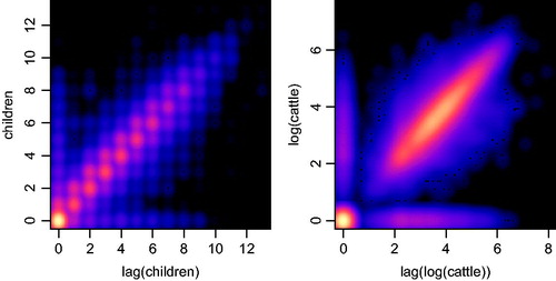
Another way to assess the quality of the created panel is to inspect the correlation of variables within linked households over time (Figure 6). To check the correlations over time, we compare the number of settler children (children who are not Khoesan or slaves) and cattle on the farms with their respective one year lags. As expected, it can clearly be seen that the panel displays a strong correlation between the variables and their lags (Pearson correlation coefficient is 0.9 for the number of settler children and 0.83 for the number of cattle).¹³

Figure 6. Smoothed scatter plot of the number of children v. the one year lag of number children (left) and of the natural logarithm of the number of cattle v. its one-year lag (right) in panel created through record linkage.

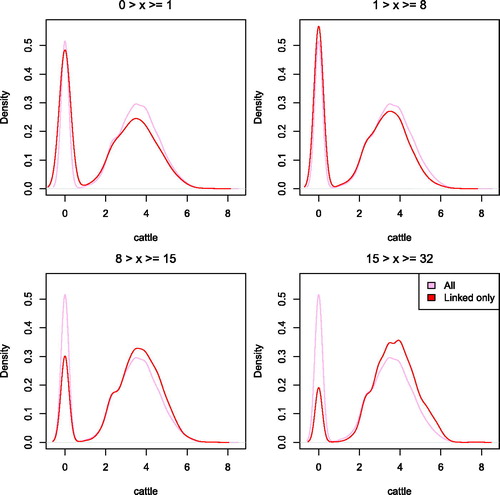
Differences in the data between the linked and unlinked observations can reveal if there are any biases in the resulting data, as well as provide a check on the characteristics that drive the record linkage procedure (that is: are the biases as we expect them to be?). Figure 7 shows the distribution of the number of cattle owned per household broken down by the length of the created series. It can be seen that the distribution for short series is similar to the one for unlinked households. However, longer linked series show fewer households with no cattle (the spike at the left) and in the case of the longest linked series (bottom right panel), more households with a high number of cattle. One possible reason for this pattern is that households with a high number of cattle were less likely to migrate compared to households without such valuable assets. They are therefore more likely to be captured by our linkage procedure for Graaff-Reinet. In general, wealthier families in the opgaafrolle are more likely to have characteristics that make them easier to link. Moreover, rare surnames are easier to link and can also be informative of economic outcomes (Guell, Mora, and Telmer 2015; Clark et al. 2015). Besides this general phenomenon, it is particularly important in our case that household heads with large farms were also more likely to be married (households with a wife present on average had more than twice as many cattle in Graaff Reinet), thus increasing the proportion of links through the information contained in the wives’ names.

Figure 7. Distribution of natural logarithm of number of cattle by length of series. x refers to the series length.

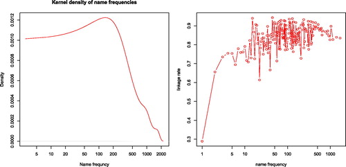
To deal with these biases, we follow Goeken et al. (2011) and provide weights based on the inverse of the linking rate of variables showing a strong linking gradient. We have considered two weighting variables: one based on the presence of a wife (indirectly capturing marital status), and one on the name frequency. The weight based on the presence of a wife is probably the most important as it strongly predicts linkage (linkage rates are 87% versus 72%) and is probably correlated with many outcomes of interest (Solon, Haider, and Wooldridge 2015). Surname frequency shows a strong gradient at frequencies lower than 10, with rarer surnames less likely to be linked (see Figure 8). Above 10, no linkage gradient can be observed. Altogether, this means that rare surnames are not improving our linkage rates, but rather only capture the fact that some names were so infrequent that they were unlikely to be linked. Moreover, name frequency is probably not as highly correlated with outcome variables of interest as the presence of a wife. We therefore suggest that the presence of a wife is the most important linking variable.¹⁴ Finally, because the panel contains the unlinked individuals as well as all the variables used to construct the links, users of the data can create further weighting variables to meet the specific requirements of their analyses.

Figure 8. Distribution of uniformised name frequency in the Graaff Reinet district and linkage rate by name frequency. Name frequency is plotted in a logarithmic axis. Distribution computed using kernel density estimation, a nonparametric method to estimate the probability density function. The linkage rate is the share of observations in the opgaafrolle data that was linked to the genealogy dataset.

While our linked dataset is not without biases, we have been able to create a model that provides high recall and precision links. The sensitivity and precision of the model on the training and test data are high and at more than 80% the overall linkage rate on the complete data is also high (Massey 2017; Feigenbaum 2016). This is especially striking given the fact that the opgaafrolle lack a number of the conventionally important variables for record linkage such as age or place of birth. The transcription of names is not the reason for our high linkage rate. Small spelling variants between the names from one year to the next are frequent. We also do not think the naming practices in South Africa are to credit. Figure 8 shows the distribution of surnames over our entire panel as well as the linkage rate by frequency. It can be seen that linkage rates are not higher for rare names.

The reason we are able to achieve high linkage rates with a low number of false positives despite the existence of common surnames is that we also use other household information to make the links (see also Fu et al. 2014). While a surname and a first name of the husband are often unable to provide an unambiguous link, adding the first name and surname of the wife often does allow us to make that distinction. Figure 4 confirms this: 1801 and 1803 are years in which the wives’ names are only recorded infrequently in the opgaafrolle and our linkage rate drops to just over 60%, in line with individual-level historical record linkage strategies. Additionally, the fact that our data are close to annual means that events such as migration, death, or changes in the composition of the household are less frequent in adjacent years than in datasets with a greater time gap. This will also increase linkage rates.

Linking External data: South African Families

Thus far, our record linkage efforts have used relatively consistent source material: the various years of the opgaafrolle. Most information in one year is usually also present in the next. However, many record linkage tasks will have to deal with more heterogeneous data. The data in the opgaafrolle also lack certain information that would be useful for analyses. Most importantly, it is lacking demographic data as no ages, dates of marriage, details on childbirths, or family links are provided. The latter would allow us to know the composition of the households in more detail and also provide insight into intergenerational mechanisms of economic success.

For these reasons, we also attempt to link the opgaafrolle to an outside dataset. One such source is a large genealogical database of the South African settler population, South African Families (SAF, see Cilliers 2016). SAF is a complete register of European settlers and their descendants at the Cape spanning over 250 years from settlement in 1652 to the beginning of the twentieth century. Unique in its size and scope across time and space, it offers a longitudinal account of individual life histories of white settlers.

Linking this dataset to the opgaafrolle requires some modifications to our strategy used to link within the opgaafrolle. These modifications concern the creation of a linkage window to prevent having to match against a large number of implausible candidates and dealing with the fact that we cannot recreate all the opgaafolle variables in the SAF-data. Other than these modifications, we have used the same procedure as outlined above.

Information contained in the genealogies includes names of all family members (also maiden names of wives), dates and locations for birth, baptism, marriage, and death, as well as occasionally occupations. However, not all entries contain complete information for every event. While close to two-thirds of the entries contain a birth or a baptism date, only one quarter contain a death date, and less than one-fifth contain a marriage date. Nevertheless, these dates, where available, allow for an additional selection step, in which individuals in the genealogies who could not possibly be a match to the opgaafrolle given their birth and death dates can be excluded.¹⁵ This is important for the prevention of false negatives as well as computational feasibility given the size of SAF. We use the date-of-death of the husband (after the year of the opgaafrol, but no later than 100 years after) and date-of-birth (16 years before the year of the opgaafrol tax, but no earlier than 100 years before) to construct our linking window. This step reduces the size of potential matches from over 670,000 (the full SAF database), to 153,156. Date-of-death and date-of-birth are, however, often missing (119,548 and 110,232 observations, respectively). Further selection based on the date of birth of children in a household reduces the number of individuals in SAF further. We include men whose children were born between 48 years before the year of the opgaafrol (meaning a male fathering a child at age 12 would be 60 at the time of the opgaafrol) or 88 years after the year of the opgaafrol (a male household head aged 12 at the time of the opgaafrol could conceivably still father a child at that time).

Because some of the variables are not available or would not contain a great deal of information in SAF, the full random forest classifier, we use to predict linkages within the opgaafrolle cannot be used here. One set of variables we exclude are cross-spouse surname string distances. In the within-opgaafrolle linking, these variables were meant to capture year-to-year variation in wife’s surname—especially whether the wife had dropped her maiden name. But since wives are reported only once with their maiden name in the genealogies, such a distance measure would have no meaning in the linking between SAF and the opgaafrolle. We have also excluded the old and young dummies since it is unclear when a person in the opgaafrolle qualified as either, making it difficult to construct a similar variable for the genealogies. The order of the observations is also excluded. This was meant to capture the order in which households were recorded in the opgaafrolle, which has no equivalent in the genealogies. Also excluded were the wine producer and district dummy variables.

This model was trained and evaluated on the opgaafrolle training data (that is: no new training and test data were created for the SAF-to-opgaafrolle linkage). While this model has to work with less information, it still performs well on the opgaafrolle training data. Ninety-six percent of the true matches are correctly classified in the training data and 87% of the true matches are correctly classified in the test data, similar to the results of the full model (99% and 86%). The number of false negatives on the test data (14) is also comparable to the full model. The fact that the name distances are the most important predictor variables in the original model explains why the model’s predictive power deteriorates only slightly while omitting a number of variables.

We select the best match from the genealogies for each person in each year. Because the opgaafrolle have already been linked over time, this allows for the possibility that the same opgaafrol-person over time (according to our linkage procedure) gets linked to multiple genealogy-persons. Reassuringly, this does not happen often (1,729 out of 21,496 linked individuals in the opgaafrolle). We chose to drop these links to the genealogies altogether. However, it would probably be possible to disambiguate a few of these links. Figure A1 in the appendix shows that the differences of the mean linking scores of the doubly linked persons can be substantial. While the largest differences can probably be resolved, developing a systematic rule would require a new training data set which is beyond the scope of this article.

The share of observations in the opgaafrolle that our procedure managed to link is shown in Figure 9. Again, it shows that in the years where the names of the wives are usually absent (1801 and 1803), linkage is difficult. Elsewhere, the share of observations matched is fairly high in the latest years (about 55%), but decreases to below 40% as we go further back in time. One reason for this is that the number of persons in the genealogies increases exponentially over time as a result of population growth and continued immigration (Cilliers 2016), so the further back in time we try to link, the smaller the number of candidates will be. Overall, it is feasible to scale the procedure to larger datasets.

Figure 9. Share of observations in opgaafrolle that is linked to an observation in the genealogy by year.

Overall, the efforts to link the opgaafrolle to the genealogy data have been successful in two ways. First, it adds valuable demographic data to the economic information contained in the opgaafrolle panel. We are hopeful that additional supplementary data can be linked to the final panel as well. Second, it shows that our linkage strategy is more widely applicable than to the opgaafrolle alone. We think that any household-level data that contain the surnames and first names of the husband and the wife and uses the naming conventions of South Africa in the eighteenth and nineteenth century (a mix of Dutch, English, German, and French) could potentially be linked using our strategy and classifier. Creating additional training data for these datasets could improve performance further.

Scalability

While we are generally satisfied with our record linkage procedure, a few issues with scalability remain. Memory usage is especially an issue because we have to use string distances for our blocking strategy. By comparing one base year of observations with the rest of the dataset rather than all observations at once, we have already limited the computational burden this imposes. Rather than a 13 GB object containing all the string distances that we would get if we compare all the 42,354 male surnames at once, we are now left with an object smaller than 1 GB. This means that the creation of each distance matrix takes less than a minute on commodity hardware.¹⁶

Once we begin to expand the dataset, however, computation may become more difficult. Currently, the Graaff-Reinet opgaafrolle contain 42,354 observations, spread over 35 years and 1–14 sub-districts (depending on the year). The eventual goal of the Cape of Good Hope Panel project is to cover 150 years for each of the territories that make up the Cape Colony. If we take an upper limit to the comparison depth of 60 years and restrict ourselves to within-district linkage, this should still keep the size of the candidates string distance matrix, currently our most computationally intensive step in the procedure, below 1.5 GB.

However, computing difficulties might arise as the project expands. Neighboring territories are one such complication. Borders were not stable, so we can expect to find households appearing in different territories in later years even if people did not migrate. This could increase the number of records that needs to be considered, though a detailed graph of neighboring sub-districts or districts would help. Should we want to follow migrants in the panel, record linkage will become more computationally expensive as well. This means we would have to search for ways to make our record linkage more scalable. Options to do this include: using a different indexing method (blocking) for candidate selection, parallelization of string distance matrix calculation, parallelization of string comparisons, and parallelization of estimation of the random forest model and its predictions.

Conclusion

This article has explained the record linkage strategy used to create the Cape of Good Hope Panel. The basis for this panel are the opgaafrolle, annual census returns for settlers of the Cape Colony, an area at the southern tip of Africa settled by Europeans in the seventeenth century. The tax censuses contain valuable information on agricultural production and demographic characteristics of the settlers. To get the most out of these censuses, it is necessary to create a panel by linking the households in the repeated cross-sectional censuses. This article constructs a matching algorithm to link settlers residing in one region of the Cape Colony, Graaff-Reinet, for the years 1787–1828.

The first step was to manually create 441 links between 608 and 674 households across two years. From this starting point, we created linkage candidates based on the male surname string distances. This training dataset was then used to estimate a model to classify new, unlinked observations. We preferred a random forest classifier over alternative classifiers, most notably logistic regression, because it resulted in fewer false positives. The model takes on board as much information in the opgaafrolle as possible, but the string distances of the husband and wife names are the strongest predictors of a link. The training and test data show that our model has a sensitivity of 86% and a precision of 94% meaning that it correctly classifies 86% of the manually identified links and has an acceptable rate of false positives. A key driver of this high linkage rate is our use of household-level characteristics and near-annual data.

The number of links created in the resulting dataset is more than sufficient for most socio-economic analyses. Almost three-quarters of the dataset consists of series of at least three observations per individual and nearly half is of length eight or more. Moreover, the created links show the expected correlations in demographic or economic variables. It is however important to be aware of the biases that are created in the linkage process. Notably, linkage rates of households with a married couple were 20 percentage points higher, skewing the subset of the longest series (length eight or more) compared to the overall dataset. Weights are provided in the data to correct for this issue in analyses.

We have also explored the possibilities of linking the Cape of Good Hope Panel to a genealogical database (SAF). The SAF adds valuable demographic information to the opgaafrolle. Matching is done using the same training data and random forest classifier as for the within-opgaafrolle linkage task, but using fewer variables to match the variables in the genealogical data. Nonetheless, 87% of the links are correctly identified in the test data and this allows us to link a person from the genealogies to half the households in the opgaafrolle. This means our approach is more generally applicable and should enable us to create a more detailed and complete dataset of Cape Colony settlers.

We expect our method to be able to scale beyond Graaff-Reinet, the district we analyzed here. If we want to follow households across districts, however, it will be necessary to compare far more records at once. Memory usage would especially become a concern and for this reason, a better blocking procedure than male surname string distance will be necessary.

Table 1. Example records from Graaff-Reinet opgaafrolle.

Year	mfirst	mlast	wfirst	wlast	old	…
1828	dirk jacobus	coetzee	engela geertruida	grobler	0	…
1828	jan willem	mienie	anna maria	els	0	…
1828	alewijn petrus johannes	van heerden	anna willemina hendrina	lubbe	0	…
…	…	…	…	…	…	…
1826	johannes willem	minnie	anna maria	els	0	…
…	…	…	…	…	…	…
1824	dirk jacobus	koetzee	engela geertruida	grobler	0	…
…	…	…	…	…	…	…

Notes

1 The R scripts (R Core Team 2015) for the procedure can be found at https://github. com/rijpma/opgaafrolle/.

2 This was done because we did not expect accents to be consistently applied between census years.

3 The administrator of the census would sometimes append a name with junior or old or, in rare occasions, deceased. This is, ostensibly, to identify men of the same name—most frequently fathers and sons, living in close proximity to one another.

4 We experimented with other ways of capturing order information, especially using the string distance of shifted observations, but these did not improve the model’s performance.

5 We also tried to use separate models for observations with and without the wives’ names to make sure that the importance of the wives’ names did not hinder our ability to make links where the wife was absent. However, the minor improvement in performance did not compensate for the additional complexity of having to create matches from two different models.

6 The surname frequency was calculated on the basis of the entire Graaff-Reinet corpus. We used uniformized surnames to avoid giving each minor spelling variation a separate count since these variations could be transcription error. Uniformization was done by aggregating surnames that had a Jaro–Winkler string distance of 0.2 or less. Note that this uniformization procedure was not used in the direct string comparisons of names, but only for the creation of this surname frequency variable. In this respect, our approach differs from that of Vick and Huynh (2011).

7 The random forest classifier is an extension of the decision trees classifier which repeatedly segments the data to predict outcomes. Random forest lowers the variance of decision trees by averaging over a large number of trees, each based on a subset of the predictor variables to decrease the correlation between the trees (James et al. 2013).

8 With precisions of 91% and 92%, the support vector machine and neural net classifiers also performed worse than the random forest model.

9 For example, a low string distance between the men’s first names should be required if there is a large string distance between the wives’ surnames (due to remarriage or a change from maiden name to husbands name).

10 Weights: mlastdist 0.27; mfirstdist 0.16; minidist 0.05; winidist 0.03; wlastdist 0.14; wfirstdist 0.07; mlastsdx 0.11; mfirstsdx 0.05; wlastsdx 0.05; wfirstsdx 0.03; mtchs 0.03. Note that this manual weighting was also done on the male surname distance-blocked candidates, so our manual weighting of the male surname distance was very high relative to the informativeness of the variable as indicated by the model-based procedure. Other weighting schemes were tried, but performance was generally similar or worse, showing that it is difficult to guess the actual informativeness of the variables.

11 The sensitivity on the test data of the support vector machine (Venables and Ripley 2002) and a neural net classifier (Meyer et al. 2017) was 86% and 85%, respectively.

12 We were not able to test the exclusion of every combination of variables because more than 8 million combinations are possible.

13 This also suggests that serial correlation will be an important issue when analyzing the data.

14 We do however provide weights based on four categories of name frequencies (1, 2–5, 6–10, greater than 10) in the final dataset.

15 Since the opgaafrolle for Graaff-Reinet only cover the period 1787-1828 and SAF spans 1652-2012 there are many individuals in SAF that could not possibly be a match to an individual in the opgaafrolle given that some will already be dead before the opgaafrolle begin, while others will not have been born until long after the opgaafrolle end. We therefore only consider SAF-persons who were conceivably alive during the opgaafrolle period.

16 Of course, such a matrix needs to be created as many times as there are base years, so there is no advantage in processing time to doing the procedure one year at a time. However, the advantage of keeping the base years separate for memory limits is substantial.

Appendix

Figure A1. Distribution of between-group linking scores. For each indexed person in the opgaafrolle that was linked to more than one person from the genealogies, the difference of the mean random forest classification score for each genealogy-person was calculated. The maximum possible difference is 0.5.

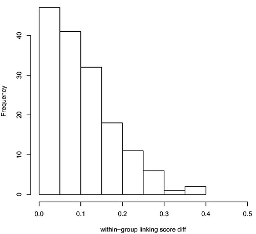
Table A1. Logistical regression predicting record matches.

	Model 1
(Intercept)	10.24	(3.76)	**
wifepresent_from	3.79	(0.73)	***
spousenamedist_from	1.71	(1.20)
namefreq_from	−0.12	(5.23)
wifepresent_to	2.94	(0.83)	***
spousenamedist_to	1.95	(1.48)
namefreq_to	0.67	(5.24)
mlastdist	0.81	(1.23)
mfirstdist	−6.16	(1.89)	**
minidist	−4.49	(0.97)	***
wlastdist	−13.45	(4.62)	**
wfirstdist	2.86	(2.37)
winidist	−4.24	(1.16)	***
mlastsdx	−1.30	(1.12)
mfirstsdx	0.25	(0.54)
wlastsdx	−0.88	(1.61)
wfirstsdx	−1.94	(1.02)
wifeinboth	−12.52	(3.46)	***
dchildren	0.90	(1.79)
mtchs	−2.66	(1.07)	*
AIC	281.1
BIC	405.33
Log Likelihood	−120.55
Deviance	241.10
Num. obs.	3683

***p < .001, **p < .01, *p < .05

Table B2. False positives created by random forest classifier.

mlast_from	mfirst_from	wlast_from	wfirst_from	mlast_to	mfirst_to	wlast_to	wfirst_to
Kunhl	p. f.	godier	j.	kluhl	petrus francois	godier	maria
Konkel	johannes lodewicus	otto	maria aletta	kinkel	johannes lucas	otto	maria aletta
Greef	matthys johannes			greef	matthys johannes
du prees	johannes francis			du preez	johannes fredericus
Loots	paul johannes jacobus			loots	paul johannes jacobus
Burger	andries petrus			burger	andries petrus
claassen	johannes hendrik			klaassen	jan henddrik
Brits	rudolf johannes	du toit	maria catharina	brits	rudolph johannes	du toit	maria catharina
Brits	rudolf	brits	elzie sophia	brits	rudolph	brits	elsje
combrink	michiel			combrink	michiel
Leroux	jan hendrik	viljoen	m. christina gertruida	le roux	jan henddrik	viljoen	maria christina geertruida
liebenberg	christoffel johannes	van der merwe	anna maria	liebenberg	charel johannes	van der merwe	anna maria

Table A3. AUC after omitting one variable.

V1	AUC
minidist	0.93
wlastdist	0.93
wfirstdist	0.93
wlastsdx	0.93
winidist	0.93
wfirstsdx	0.93
bothyoung	0.93
bothwineprod	0.93
spousenamedist_from	0.94
wifepresent_from	0.94
wifepresent_to	0.94
spousenamedist_to	0.94
mfirstdist	0.94
correct	0.94
mlastdist	0.94
dchildren	0.94
namefreq_to	0.94
mlastsdx	0.94
wifeinboth	0.94
mtchs	0.94
nrdist	0.94
mfirstsdx	0.94
bothold	0.94

Table A4. AUC after omitting two variables (full model AUC: 0.94).

V1	V2	AUC
mfirstdist	minidist	0.90
minidist	wlastsdx	0.91
wlastdist	wlastsdx	0.91
minidist	mtchs	0.92
minidist	winidist	0.92
minidist	wlastdist	0.92
minidist	wfirstsdx	0.92
correct	minidist	0.92
minidist	mlastsdx	0.92
wifepresent_from	winidist	0.92
wifepresent_to	winidist	0.93
minidist	wifeinboth	0.93
spousenamedist_to	minidist	0.93
namefreq_to	minidist	0.93
winidist	wlastsdx	0.93
wifepresent_from	wifepresent_to	0.93
wifepresent_from	minidist	0.93
minidist	wfirstdist	0.93
wfirstdist	winidist	0.93
spousenamedist_from	minidist	0.93

Note: only 20 lowest AUC values reported.

References

- Antonie, L., K. Inwood, D. J. Lizotte, and J. Andrew Ross. 2014. Tracking people over time in 19th century Canada for longitudinal analysis. Machine Learning 95(1):129–46. no. :
- Bloothooft, G., P. Christen, K. Mandemakers, and M. Schraagen. 2015. Population reconstruction. Cham: Springer.
- Breiman, L. 2001. Random forests. Machine Learning 45(1):5–32.
- Christen, P. 2012. Data matching: Concepts and techniques for record linkage, entity resolution, and duplicate detection. Berlin: Springer Science & Business Media.
- Cilliers, J. A. 2016. “A demographic history of settler South Africa.” Thesis, Stellenbosch University. http://ir.nrf.ac.za/handle/10907/497.
- Clark, G., N. Cummins, Y. Hao, and D. D. Vidal. 2015. Surnames: A new source for the history of social mobility. Explorations in Economic History 55(1):3–24.
- Dong, H., C. Campbell, S. Kurosu, W. Yang, and J. Z. Lee. 2015. New sources for comparative social science: Historical population panel data from East Asia. Demography 52 (3):1061–88.
- Feigenbaum, J. J. 2016. “Automated census record linking: A machine learning approach.” http://scholar.harvard.edu/jfeigenbaum/publications/ automated-census-record-linking.
- Ferrie, J. P. 1996. A new sample of males linked from the public use microdata sample of the 1850 U.S. Federal census of population to the 1860 U.S. Federal census manuscript schedules. Historical Methods: A Journal of Quantitative and Interdisciplinary History 29(4):141–56. no. : https://doi.org/10.1080/01615440.1996.10112735.
- Fourie, J. 2016. The data revolution in African economic history. Journal of Interdisciplinary History 47 (2):193–212.
- Fu, Z., H. Boot, P. Christen, and J. Zhou. 2014. Automatic record linkage of individuals and households in historical census data. International Journal of Humanities and Arts Computing 8(2):204–25. no. :
- Goeken, R., L. Huynh, T. A. Lynch, and R. Vick. 2011. New methods of census record linking. Historical Methods: A Journal of Quantitative and Interdisciplinary History 44(1):7–14. no. : https://doi.org/10.1080/01615440.2010.517152.
- Guell, M., J. V. R. Mora, and C. I. Telmer. 2015. The informational content of surnames, the evolution of intergenerational mobility and assortative mating. The Review of Economic Studies 82(2):693–735.
- Hastie, T., R. Tibshirani, and J. H. Friedman. 2009. The elements of statistical learning: data mining, inference, and prediction. Second edition, corrected 7th printing. Springer series in statistics. New York: Springer.
- Hautaniemi, S. I., D. L. Anderton, and A. Swedlund. 2000. Methods and validity of a panel study using record linkage: Matching death records to a geographic census sample in two Massachusetts towns, 1850– 1912. Historical Methods: A Journal of Quantitative and Interdisciplinary History 33(1):16–29. no. : Accessed June 28, 2018. https://doi.org/10.1080/01615440009598943.
- Heckman, J. J. 1979. Sample selection bias as a specification error. Econometrica 47(1):153–61.
- James, G., D. Witten, T. Hastie, and R. Tibshirani. 2013. An introduction to statistical learning. Vol. 6. New York: Springer.
- Liaw, A., and M. Wiener. 2002. Classification and regression by random-forest. R News 2(3):18–22. http://CRAN.R-project.org/doc/Rnews/.
- Little, R. J., and D. B. Rubin. 1987. Statistical analysis with missing data. New York: Wiley.
- Loo, M. P. J. V D. 2014. The stringdist package for approximate string matching. The R Journal 6(1):111–22. http://CRAN.R- project. org/package = stringdist.
- Massey, C. G. 2017. Playing with matches: an assessment of accuracy in linked historical data. Historical Methods: A Journal of Quantitative and Interdisciplinary History 1–15. doi.org/10.1080/01615440.2017.1288598
- Meyer, D., E. Dimitriadou, K. Hornik, A. Weingessel, and F. Leisch. 2017. e1071: Misc Functions of the Department of Statistics, Probability Theory Group (Formerly: E1071), TU Wien. https://CRAN.R-project.org/package=e1071.
- Potgieter, M., and J. Visagie. 1974. Inventaris van Opgaafrolle. Cape Town: Cape Town Archives Repository.
- R Core Team 2015. R: A language and environment for statistical computing. Vienna, Austria: R Foundation for Statistical Computing. https://www.R-project.org/.
- Rosenwaike, I., M. E. Hill, S. H. Preston, and I. T. Elo. 1998. Linking death certificates to early census records: the african american matched records sample. Historical Methods: A Journal of Quantitative and Interdisciplinary History 31(2):65–74. Accessed June 28, 2018. http://www.tandfonline.com/doi/abs/10.1080/01615449809601189.
- Ruggles, S. 2002. Linking historical censuses: A new approach. History and Computing 14(1–2):213–24. Accessed June 28, 2018. https://www.euppublishing.com/doi/abs/10.3366/hac.2002.14.1-2.213.
- Ruggles, S. 2012. The future of historical family demography. Annual Review of Sociology 38(1):423–41. http://dx.doi.org/10.1146/annurevsoc- 071811-145533.
- Ruggles, S. 2014. Big microdata for population research. Demography 51(1):287–97.
- Ruggles, S., C. A. Fitch, and E. Roberts. 2018. Historical census record linkage. Annual Review of Sociology 44 (1)null. Accessed June 28, 2018. https://doi.org/10.1146/annurev-soc-073117-041447.
- Solon, G., S. J. Haider, and J. M. Wooldridge. 2015. What are We weighting for? Journal of Human Resources 50(2):301–16. no. :
- Venables, W. N., and B. D. Ripley. 2002. Modern applied statistics with S. Fourth. New York: Springer. http://www.stats.ox.ac.uk/pub/MASS4.
- Vick, R., and L. Huynh. 2011. The effects of standardizing names for record linkage: Evidence from the United States and Norway. Historical Methods: A Journal of Quantitative and Interdisciplinary History 44(1):15–24. no. : http://dx.doi.org/10.1080/01615440.2010.514849.
- Wisselgren, M. J., S. Edvinsson, M. Berggren, and M. Larsson. 2014. Testing methods of record linkage on Swedish censuses. Historical Methods: A Journal of Quantitative and Interdisciplinary History 47(3):138–51. no. : https://doi.org/10.1080/01615440.2014.913967.