A new strategy for linking U.S. historical censuses: A case study for the IPUMS multigenerational longitudinal panel

Abstract

This paper presents a probabilistic method of record linkage, developed using the U.S. full count censuses of 1900 and 1910 but applicable to many sources of digitized historical records. The method links records using a two-step approach, first establishing high confidence matches among men by exploiting a comprehensive set of individual and contextual characteristics. The method then proceeds to link both men and women by leveraging links between households established in the first step. While only the first stage links can be directly comparable to other popular methods in research on the U.S., our method yields both considerably higher linkage rates and greater accuracy while only performing negligibly worse than other algorithms in resembling the target population.

Keywords:

• Record linkage
• United States of America
• census data
• machine learning

Introduction

A broad set of social research questions benefits from having individuals linked across datasets and time. This includes research related to demographic behavior, intergenerational mobility and how conditions during childhood affects later-life outcomes. In the United States, considerable efforts have been made to digitize vast amounts of individual level data, with the publically available full-count decennial censuses from 1850 to 1940 being the most notable example. This data opens the possibility for life-course studies across multiple birth cohorts, but the lack of a stable personal identifier (such as a Social Security number) in historical sources makes it challenging to link individuals across records.

During the past 25 years, multiple efforts have been undertaken to combine historical individual records in order to create longitudinal data, thereby allowing for an improved understanding of the past. Along with the digitization of historical records and improved computational capabilities, an acceleration of the development of computerized, automated linking methods has ensued. The main aim of the paper is to present a two-step probabilistic method of automated record linkage, developed for linking individuals across historical records using the U.S. full count censuses of 1900 and 1910. The method was developed within the Multigenerational Longitudinal Panel project at the University of Minnesota, aiming to link individuals across the 1850–1940 historical US censuses and death records. The presented method has been used to produce the public-use IPUMS MLP datasets, to date providing individual links covering the 1900–1940 decennial U.S. Federal Censuses.

Besides variables used in most record linking efforts, our method incorporates a broader set of household and neighborhood contextual features, yielding computer-generated matches closer to those a human genealogist would produce and – equally importantly – without decreasing performance for individuals lacking this data. The method begins by exploiting the broader set of characteristics to first establish high confidence links among individuals. In a second step, the method then compares all remaining household members of the original linked individuals and establishes additional links. Since the only potential matches are within the household, we are able to substantially relax the criteria which otherwise may have prevented successful linkage while at the same time maintaining very quality links. In this implementation of the method, we begin by only linking males in the first step and then linking males and females in the second, household-based step. The resulting linkages provide high quality links of individual men, couples, and some women. While implementing the full algorithm maximizes the share of the underlying population that is linked, some researchers may opt only for the implementation of the first step, most comparable with the current efforts of the Census Linking Project. This also motivates why we during this step exclusively link men, in addition to unique challenges in linking women due to surname changes after marriage.

Advances in record linkage during the past decade imply that researchers today either can choose between already linked data generated using different methods, or – if conducting their own record linkage –between several carefully outlined linking algorithms to implement themselves. A second aim of this paper is therefore to compare how the method outlined in this paper compares to the methods that today are most commonly encountered in the scientific literature within the U.S. context. While this comparison necessarily is limited to the first stage of our algorithm, our results suggest that we are not only able to achieve a match rate that is twice as high and with higher precision and out-of-sample accuracy than other popular methods, in addition to obtaining a linked sample which performs almost equally well in terms of resembling the target population. While the method outlined in the paper has been developed for linking individuals across decennial U.S. censuses, its underlying principles can also help improve the linking of other datasets in which individuals are listed along with their family members or neighbors.

Background: Earlier record linkage efforts

Efforts to create longitudinal individual data for historical populations, frequently exploiting numerous different types of source material, are by no means novel. Examples from across the world include longitudinal datasets from Sweden (Scanian Economic Demographic Database, POPLINK), Canada (BALSAC), the Netherlands (Historical Sample of the Netherlands) and China (China Multi-Generational Panel Datasets), allowing for the study of demographic and socioeconomic outcomes from a life-course perspective over time periods, and in some cases going as far back in time as the 17th century while they reside in the area in question.

Record linkage of historical U.S. censuses began as early as Malin (1935) who linked farm operators in Kansas across thirteen censuses taken between 1860 and 1935. All early census record linkage was limited to smaller geographical areas such as Trempeleau county, Wisconsin (Curti 1959), Newburyport, Massachusetts (Thernstrom 1964), Atlanta, Georgia (Hopkins 1968), Boston, Massachusetts (Knights 1971) and Kingston, New York (Blumin 1976). The overarching linking methodology in these studies was to track a population of men over time by manually searching microfilmed census listings. Since their source material only covered the location where the sample population was first observed, the study population became restricted to individuals who did not migrate, with nontrivial consequences regarding representability of the resulting sample (Ruggles, Fitch, and Roberts 2018).

While constant human supervision over the linking process is an advantage, there are also many disadvantages. The true characteristics of the individual in the record are often altered by reporting errors from the respondent, errors introduced by the enumerator, and transcription errors in converting the hand-written text into machine-readable format. Given these sources of errors, the decision of whether individuals in two records are the same person often involves weighing a complicated set of factors. As a consequence, it is difficult for manual linkers to maintain consistent criteria for determining matches. It is difficult to fully document the decision process, making replication impossible. Beyond the concerns about validity and reliability, manual record linkage is time consuming and expensive, making it infeasible for large populations that extend beyond local areas.

As earlier attempts to track individuals over time using U.S. data relied on source material with limited opportunities to sort, restrict, and search among records, the first release of IPUMS data in the early 1990s represented a watershed moment. The digitization of historical census records opened new opportunities to examine and follow substantially larger populations over time, catalyzing the transition to computerized approaches for processing the data. With the availability of larger population sets, one major challenge associated with linking census data became obvious: how could one systematically and most effectively use the available information in the source material to find the records corresponding to the same individual in another source? Theoretically, this is a straightforward task, as we expect individuals to carry certain immutable characteristics over their lifespan. For example, an individual named John Smith, male and born in state s in the year t will display these same characteristics in the next census. Defining the universe of potential matches would therefore represent a straightforward task, limiting the population to individuals sharing those characteristics. However, several factors make this less straightforward, including the prevalence of proxy reporting¹ and lack of detail and precision in the data. As a result, nontrivial differences in the spelling of names and in the reported year or state of birth are common. This presents the researcher with a dilemma, since while allowing for a widely defined universe of potential matches increases the probability that the true match will be among the potential matches, it also increases the risk of false positives as well as increasing computational requirements. For example, going from restricting potential matches to individuals reporting the same year of birth to instead allowing for birth year reporting error of +/- three years increases the amount of potential matches (amount of data that needs to be processed) by 900 percent, holding everything else constant.

An early use of IPUMS for linking U.S. census data was made by Ferrie (1996), whose approach originated from a set of rules based on which records across two different censuses were considered to be the same person. Ferrie exploited the IPUMS sample for 1850 and an alphabetic name index of the 1860 census that had been constructed for genealogical use. Ferrie coded both the IPUMS data and the 1860 index phonetically and searched the 1860 index for cases that phonetically matched each name in the IPUMS sample. After discarding cases with more than 10 potential matches, Ferrie located each potential match on the microfilm of the census enumeration, and used birth year (within three years), state or country of birth, and the presence of family members to determine which match was correct. If there were two or more perfect matches the individual with the closest age difference was selected.

At a meeting on historical record linkage held at the University of Montreal in 2003, Ruggles (2002) argued that using information about family members, place of residence, or occupation to disambiguate potential links would introduce selection bias that would be likely to distort estimates of geographic or economic mobility and other life-course transitions. Ferrie had come to a similar conclusion, and he announced that he had already embarked on a new fully-automated record linkage project using only characteristics that in theory should remain consistent over time: name (for males), age, sex, and birthplace.

Ferrie’s fully-automated record linkage became feasible with the advent of the first full-count historical census microdata. In 2003, a collaboration of IPUMS and The Church of Jesus Christ of Latter-day Saints released census microdata covering the entire U.S. population enumerated in 1880, comprising over 50 million records (Roberts et al. 2003). Ferrie (2005) linked the new 1880 full-count database to the IPUMS 1% samples of the 1850, 1860, 1870, 1900, and 1910 censuses. To avoid selection bias, Ferrie considered a limited set of variables. He required an exact match on name (except for very small spelling variations), matching birthplace, and a birth year within three years. All multiple matches were dropped, and no information on family members, place of residence, or other variables was consulted.

Subsequent efforts to link U.S. censuses have virtually all followed Ferrie’s lead and avoided the use of variables that could introduce selection biases. IPUMS linked the 1880-full count census to the other IPUMS samples using the same variables as Ferrie, but using a probabilistic machine-learning strategy instead of his deterministic approach. The IPUMS Linked Representative Samples (IPUMS-LRS) used a support vector machine to obtain the predicted probability that two records are a true match, based on a set of characteristics believed to be time-invariant across the life course, as well as consistently being available in both sets of data that were being linked (Goeken et al. 2011). The support vector machine used manually linked input data to calibrate the relative importance of each examined characteristic, using characteristics such as name commonality, first and last name similarity score, and age difference. This probabilistic method of record linkage thereby allows for a more flexible linking approach, but also one whose performance ultimately will depend on the accuracy of the input data used by the algorithm to recognize patterns in the data that is consistent with a pair of records referring to the same individual. After the identification of primary links, the method proceeded to link additional household members, again conditional on the same set of linking characteristics. Under the umbrella of IPUMS-LRS, multiple datasets were released, spanning the time period 1850–1930, with versions of the method also being applied to census data from other countries.

In recent years, automated linkage of U.S. censuses has become increasingly common. Many studies adapted and scaled Ferrie (1996) for use with the full-count census records that made the linking replicable, fully automated, and transparent. The first paper to implement this type of census linking for the entire population was Abramitzky, Boustan, and Eriksson (2012) and a similar approach was used by Abramitzky, Boustan, and Eriksson (2014), Collins and Wanamaker (2015), Beach et al. (2016), and Alexander and Ward (2018). In general, these studies combine the use of phonetic classification used in Ferrie (1996) with the rules introduced by Ferrie (2005). Recent work uses statistical algorithms such as expectation maximization to determine which links are correct (Abramitzky, Mill, and Pérez 2020). The code needed to implement these approaches are now widely available for researchers to use (censuslinkingproject.org) and have become a very important tool for linking historical records.

Following the example of IPUMS-LRS, other investigators have turned to probabilistic machine-learning approaches. Feigenbaum (2016) adapted a regression model to training data using statistical software and methods that are in the wheelhouse of many social scientists in order to evaluate potential matches in his 1915 Iowa sample, linked to the 1940 Census. His approach made record linking methods that employ machine learning more accessible and more understandable. Other efforts to link historical records using supervised machine learning methods include Bailey (2018), Abramitzky et al. (2020); and Price et al. (2021). The precision of each of these approaches is based on the training data that can be used to teach the model and the machine learning algorithm to discern between true and false links. Bailey et al. (2020) provides a description of a massive effort to create training data using humans to label true and false links between historical records that involve frequent standardized training and double and triple entry practices to ensure a high level of quality. Price et al. (2021) uses links created on a public genealogy platform to create training data in which high quality links are created by people doing family history for their relatives and using information that goes beyond the fields contained in the census records.

In the wake of the emergence of several straightforwardly applicable, methods of record linkage and the availability of a plethora of digitized individual level historical data, the focus has shifted toward comparing how existing methods perform. There is considerable debate about the quality of links created through automated methods (Bailey et al. 2020; Abramitzky et al. 2020). Bailey et al. (2020) uses the large training set that they created to evaluate the quality of automated linking methods. They note that 15 to 37 percent of the links created by automated methods are identified as false links by human reviewers. Their evaluation highlights the importance of comparing the predictions of automated methods with the decisions made by humans doing the same task to evaluate possible improvements to automated approaches to link records. Hand linking individuals across records is a much too slow and expensive process to provide the primary approach, but efforts to create training data or validation sets can be used in combination with automated methods to create linked samples with high match rates and high precision.

Most recent efforts to link individuals across historical U.S. sources rely exclusively on immutable characteristics to establish links. Several investigators linking data from other countries use machine learning approaches which exploit a more extended set of characteristics. Fu et al. (2014) takes information at the household level into account through the calculation of household similarity scores, and finds that this method diminishes the number of ambiguous links and raises accuracy. Rijpma, Cilliers, and Fourie (2020) use household level characteristics to identify links rather than as a way to disambiguate once primary linking is performed. This method yields considerable gains in the linkage rate while minimizing the false positive rate. Using Canadian data, Antonie et al. (2014) employ household-level characteristics in the training data generation process. Also using (potentially) time varying characteristics in the linking stage on 19th century Canadian census data, Antonie et al. (2020) find a doubling of linkage rates with trivial cost in terms of increasing the bias in the composition of the linked population. Implementing their algorithm on 19th century Canadian census data, the authors find a doubling of linkage rates with trivial cost in terms of increasing the bias in the composition of the linked population. Using Swedish census data, Wisselgren et al. (2014) implemented the IPUMS-LRS method (Goeken et al. 2011) with some minor modifications. More specifically, they examine how the implementation of the second, household-linking, stage of the algorithm affects the overall linkage rate, finding this method to improve the linkage rate considerably. A similar two-stage approach, using primary individual links to identify households as a base for straightforwardly identifying secondary links was developed by Eriksson (2015, also outlined in Dribe, Eriksson, and Scalone 2019). Lastly, the LINKS database, linking individuals across a range of civil registry certificates in the Netherlands relies on at least two pairs of names across records from different sources in order to obtain high confidence matches (van den Berg et al. 2021).

Our approach

All the early efforts to link historical records—from Malin to the first iteration of Ferrie—used all information available for linking, including the characteristics of household members. These projects generally linked only a small fraction of the population for two main reasons. First, most studies were local and lost track of out-migrants; second, the source data were not machine-readable, and it was impossible to broadly search on many characteristics to find the best possible match. Because only a small percentage of the population was linked, there was high potential for selection bias, especially bias favoring non-migrants who resided with the same family members across multiple census years. To mitigate these biases, with few exceptions, record linkage projects conducted since 2003 have tended to only rely on time-invariant characteristics, mainly name, birth year, sex, and birthplace.

In the past seven years, IPUMS has released full-count machine-readable data for every surviving U.S. census from 1850 to 1940. The availability of the full-count data opens the potential for a new approach to record linkage. A consistent feature of the U.S. historical censuses, conducted every ten years, is that information on a range of individual level demographic and socioeconomic characteristics was collected, and the information is organized into families and households. By using all the information available—mutable and immutable—we can link a far higher percentage of the population than was previously possible, with far lower levels of false links. We developed our strategy by linking individuals extracted from the 1900 census to their respective 1910 records. These censuses contain all information that we envisioned as important for the record linking algorithm,² in addition to being chronologically located approximately at the center of all the censuses to be linked within the MLP project.

Selection bias remains a concern. People who remain in the same place or remain married to the same person, for example, have more information available to establish links than do those who migrate without kin. All linkage efforts, however, introduce selection biases, and our preliminary analysis suggests that the bias introduced by our approach is comparatively small. Our linked data complements work based on linking individuals using immutable characteristics. The benefits of higher linkage rates and improved precision should be weighed against the concern of potential selection bias, particularly for social and geographic mobility.

Our approach draws on previous research in several respects, however not previously implemented in such an extensive and systematic way as here. First, we train a probabilistic machine learning algorithm to use a range of individual, household, and contextual characteristics when declaring matches. Second, we use a two-step approach, beginning by linking men in order to obtain a sample of high confidence links. We then proceed to a second step, which exploits links between households that are generated in stage one. Here, the household is used to maximally restrict the universe of potential matches, after which a second step machine learning algorithm is used to link members of those households –men and women–that were not linked in the first stage. Each stage requires a unique set of training data to calibrate its respective machine learning algorithm, outlined separately below.

Step I: Linking men

Training data

For the generation of the initial set of hand-linked training data used to calibrate the Step I algorithm, we extracted a sample of 3,000 men from the 1900 census. The training data consists of 50 randomly selected men from each state of birth (50*50 = 2500), in addition to 50 randomly selected men from 10 different regions of origin outside the United States (50*10 = 500). While deviating from the standard procedure when generating training data by not being a random draw from the underlying 1900 population of men, the sample nevertheless largely reflects the full 1900-population in terms of basic demographic characteristics, other than region of birth.

The universe of potential matches extracted from the 1910 full-count census was generated by restricting the linkable population to individuals who were male and born in the same state within +/- three years of the 1900 individual. In addition, the universe was limited to those having at least one identical last name adjusted bigram³ and a (unstandardized) first and last name Jaro-Winkler score of at least 0.7, respectively. The Jaro-Winkler threshold was set at this level in order to minimize the risk of excluding a true match from the universe of potential matches on the basis of a small name discrepancy, while at the same time maintaining a manageable universe of potential matches. Out of the 3,000 individuals initially selected from the 1900 census, the enforcement of aforementioned blocking criteria⁴ results in a population of 2,700 potentially linkable individuals. On average, the universe of potential matches for each 1900 individual amounts to 82 census records from the 1910 census, thus yielding a total training data set containing 221,388 observations.

We set out to generate training data of the highest quality possible, through systematically relying on the wealth of resources provided by Ancestry.com when evaluating each potential match. Out of the 2,700 individuals extracted from the 1900 census, we were able to confidently link 1,354 individuals, or 50.1 percent to a record among the aforementioned universe of 1910 census potential matches. The linking rate is somewhat difficult to compare to figures reported in other historical research on the United States due to differences in linking methods, samples and sources, but we remain confident that our share represents a gold standard.

Expanding the universe of linking variables

Our machine learning algorithm shares several fundamental procedural characteristics with those proposed by Feigenbaum (2016). In terms of linking variables, our linking algorithm benefits from a number of those used by Feigenbaum, while also considerably expanding the set of linking variables. Indeed, this reflects one key extension of our linking approach, proposing that data – in particular census data spanning comparatively shorter time periods – can be used more effectively and enhance the algorithm’s ability to more accurately distinguish between potential matches as outlined in greater detail below.

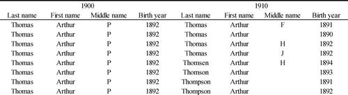
An illustrative example of the underlying idea of our proposed algorithm is provided in Figure 1, taking as a point of departure a frequently encountered situation when relying solely on individual level information. In the example, the individual to be linked, Thomas P Arthur, represents someone with a relatively common name, also translating to more than one perfect match on first and last name to individual records in the 1910 census. In a situation like this, remaining time-invariant linking characteristics are unlikely to assist in further distinguishing between the potential matches. As a result, all of the first four potential matches emerge as equally plausible candidates, with the linking algorithm thereby failing to identify one unique match. If anything, a human doing this task might choose the bottom row since the birth year matches exactly and there is no conflicting information for the middle initial.

Figure 1. Sample potential match data, only displaying (theoretically) immutable characteristics.

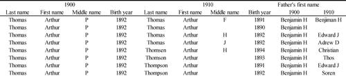
One key idea of this paper is that additional and readily available information can and should be used in order to arrive at a better calibrated machine learning algorithm. Figure 2 elaborates on the contents of Figure 1 in order to illustrate the usefulness of broadening the set of information used by the algorithm. In the example below, information on the name of the father of the 1900 individual as well as of the 1910 potential match is added, allowing for straightforwardly determining what by all accounts appear to be the correct match. In addition, it then becomes clear that the P and F for the middle initial are written in a very similar way and one of them is likely a transcription error. Indeed, while in many situations it remains very difficult to conclusively determine one potential match as the correct one, the idea underlying our algorithm is that being able to rely on additional information increases the degree of precision in doing so.

Figure 2. Sample potential match data, extended with father’s first name.

Parents and spouse characteristics

Much of the historical census population is embedded in households and families that often persist across multiple censuses. This is particularly true for children under the age of 7 and married adults who are often with at least some of the same family members ten years later.

For every record, categorical variables indicate whether the individual’s mother, father, or spouse was present in both the household of the 1900 individual and the 1910 potential match. When this is the case, the variable additionally indicates whether there is substantial mismatching information on key characteristics, suggesting that the 1900 and 1910 records are referring to a different parent or spouse. More specifically, the variable indicates the presence of (substantial) mismatch on year or place of birth, as well as whether (for the spouse) there are unrealistic values on the marriage duration variable or (for the parents) whether the parent’s relationship to the target individual changes, i.e. from biological to step-parent or vice versa. For observations where both the 1900 individual and the 1910 census potential match has a non-missing observation on the name of the family member in question, we additionally calculate the Jaro-Winkler name similarity score.

Another potentially relevant piece of information available for all individuals in the 1900 and 1910 U.S. censuses is provided by the birthplace of both the individual’s mother and father. This is operationalized as two separate indicators showing whether this matches across the censuses for the individual’s mother and father, respectively.

Other household members

Albeit less straightforward to operationalize in a manageable way, similarly useful information in accurately identifying matching records may be provided by other household members, related or otherwise. Due to individuals frequently residing in large households, we opted to operationalize the information by distinguishing between related (i.e., siblings, grandparents) and unrelated (lodgers, etc.) household members. Within each category, we calculate the Jaro-Winkler score for each member from the 1900-household and compare it to every age (+/-5 years) and sex-appropriate individual belonging to that same household member type in the potential match’s 1910 household. Thus, the Jaro-Winkler name similarity of a female relative to the 1900 index individual named “Anna” and born 1884 is calculated for all female relatives of the 1910 potential match that were born between 1879 and 1889. This ascertains that comparisons are performed between the relevant “category” of people and, furthermore, that an index individual’s uncle, born in the mid-1800s will not be compared to a potential link’s sister, born 1895, not only belonging to a different sex but also widely differing in age. Subsequent to performing all relevant comparisons, an indicator variable that is used by the algorithm is generated, signaling whether there is at least one relative of the 1900 individual whose Jaro-Winkler name similarity score is greater than or equal to 0.9 when compared to a qualifying 1910 potential match’s related household member. This threshold yields near identical name combinations allowing only minor variations in spelling. Consequently, this indicates a high likelihood that there is (at least) one common relative who resides in the same household as the 1900 individual and the potential match in 1910. An analogously generated indicator variable measures the presence of unrelated household members that are present in both records.

Residential characteristics

The censuses also contain information on the individual’s place of residence and on potentially relevant neighborhood characteristics. While not available for every household, many individuals in both censuses live in households where the street name is reported. Conditional on the 1900 index individual and the 1910 potential match individual living in the same state and county, we calculate the degree of street name similarity,⁵ again through the Jaro-Winkler string comparison score. The rationale underlying this as a linking variable pertains to its use in confirming rather than rejecting a potential match. More specifically, since migration was not uncommon, a low street name similarity score fails to provide any evidence against a potential match. On the other hand, however, a high score should provide strong evidence in favor of a match.

A second indicator is represented by calculating the share of common neighbors between the 1900 index individual and the 1910 potential match individual. Again, its main expected use is in confirming rather than rejecting potential matches, which is why we carefully design the variable only to assist with the former. We begin by extracting the ten nearest preceding and ten following household heads’ last names for the 1900 sample individual, conditional on the neighboring household residing in the same county and state as the sample individual. We follow the same procedure for the potential matching individual from the 1910 census. Thus, for an individual with at least ten households listed before and after on the census form, respectively, and residing in the same county and state, the individual’s twenty closest residing neighbors are obtained. Conditional on the 1900 individual and the 1910 potential match residing in the same state and county in both censuses, through Jaro-Winkler scores, we proceed to compare each of the 1900 individuals’ neighbors to every neighbor household’s last names of the potential match from 1910. Treating Jaro-Winkler scores above 0.95⁶ as evidence of the presence of a common neighbor in both censuses, a 1900 sample individual will have between zero and twenty common neighbors. Since the vast majority of observations pertain to individuals with either zero or several common neighbors, we operationalize this information as a dichotomous variable, indicating whether one or more neighboring household is identical across the census records.

Additional linking variables

When linking a sample of the population from one record to the full population in another record, the risk of declaring false positives will increase. An illustrative example is provided by a situation where the sample that we are trying to link contains an individual John Stevenson, born in state s and in year y. Born in the same state and year is a second John Stevenson who was not included in the random sample of the population that we chose to link. If only the second John Stevenson survived through the linking period, resulting in the linking algorithm almost certainly declaring a positive match with the namesake that was included in the linking sample. It is easy to see how this problem is exacerbated with sample data, since if we were linking full populations, both John Stevensons would likely be linked to the only surviving one. Through appropriate post-processing of the linked data, dropping duplicate links, both would be discarded from the data. In an attempt to quantify the extent of this problem for each 1900 sample individual and allowing for the algorithm to account for this, we calculate the number of individuals sharing the 1900 sample individual’s (standardized) first and last name in the 1900 census, conditional on being born in the same country/state and within +/- three years. The underlying logic is to provide the algorithm with a quantification of the likelihood that a link could be declared to another individual with the exact same name, given the aforementioned blocking criteria.

As mentioned earlier, migration at the time was common, a phenomenon that we operationalize through the distance between the county of the 1900 individual and that of the 1910 census potential match. The algorithm is also provided with information on the 1900 individual’s race, as well as whether this corresponds to the race of the 1910 potential match. The variable is intended to both capture underlying differences according to race in the ability to accurately link across censuses, as well as promoting declaring matches when the 1900 individual and the 1910 potential match are recorded as belonging to the same race. Attempting to further distinguish between individuals with different underlying linkage probabilities, the algorithm is provided with information on the 1900 individual’s region of birth, both domestic and foreign. Additionally, U.S. born individuals with (at least) one foreign born parent is additionally indicated as being second generation immigrants. Lastly, and naturally only of relevance to the foreign born, we calculate the difference in the reported immigration year for the sample individual from the 1900 census and their potential match in 1910.

Training and implementing the algorithm

The approach selected for training the machine learning algorithm is similar to Feigenbaum (2016), however relying on a logistic rather than a probit regression model as we found its performance consistently providing superior stability. Based on model parameters calibrated on training data, the machine assigns the predicted probability of a match for each 1900 and 1910 census potential match. The key decision therefore becomes which thresholds to select when declaring links in the data. This pertains to the predicted probability cutoff (α) value, roughly representing the required estimated similarity of two census records, as well as the relative probability cutoff (β) value, measuring in relative terms how much better than remaining potential matches the highest probability match is required to be. This is determined by employing a train-test-split procedure and cross-validation over a range of realistic values of both thresholds in order to identify the optimal cutoffs. The training data set is used to create ten new data sets, randomly assigning 50 percent of the observations to be the training set, with the other 50 percent being the testing set. In each data set, the algorithm was estimated on the training part, used to predict matches in the testing part of the data, subject to aforementioned values of α and β. Once matches are assigned, these are compared to the underlying verified matches in the training data, thus assigning true/false positives/negatives. Due to the varying assignment of observations to the train and test parts of the data, the performance of the algorithm will necessarily differ across datasets, holding α and β values constant. This motivates the use of ten separate train-test-split datasets, allowing us to obtain a more stable statistic by averaging over the ten observations. Selecting which α and β cutoffs to use when applying the algorithm on unseen data is not straightforward, however, as the performance parameters of interest in record linkage, precision (share of identified matches that are correct) and recall (share of matches in the underlying training data that are identified) move in opposite directions as the thresholds are adjusted.

We select α and β thresholds based on Matthew’s Correlation Coefficient (MCC), designed to be especially advantageous for use with unbalanced two-class data (Chicco 2017). The MCC, outlined in Eq. (1)(1) $$\mathit{MCC}=\mathrm{ }\frac{TP\mathrm{ }\times TN-FP\mathrm{ }\times FN}{\sqrt{(TP+FP)(TP+FN)(TN+FP)(TN+FN)}}$$(1) below, compares the predictions of the algorithm to all possible outcomes (true/false positives/negatives) and provides a single metric (ranging from −1 to +1) to be used to select which thresholds to use for overall optimal performance. For each unique combination of threshold values within a plausible range,⁷ we repeat the train-test-split procedure ten times in order to calibrate a stable MCC value. In the MCC formula displayed in Equation (1)(1) $$\mathit{MCC}=\mathrm{ }\frac{TP\mathrm{ }\times TN-FP\mathrm{ }\times FN}{\sqrt{(TP+FP)(TP+FN)(TN+FP)(TN+FN)}}$$(1) below, TP represents true positive, TN represents true negative, FP represents false positive, and FN represents false negatives: (1) $$\mathit{MCC}=\mathrm{ }\frac{TP\mathrm{ }\times TN-FP\mathrm{ }\times FN}{\sqrt{(TP+FP)(TP+FN)(TN+FP)(TN+FN)}}$$(1)

The model used to calibrate thresholds is presented in Table A1 in the Appendix, along with variable means in the underlying training data. Note that this is the model output using the full set of training data, and not the output from any of the separate train-test-split runs. Based on the average MCC obtained for each combination of α and β, we were able to identify the threshold values yielding the overall best performance, amounting to an MCC of 0.89,⁸ associated with a precision of 0.90 and a recall of 0.87.

Table 1. Linkage rate, by method.

	Step I	Feigenbaum	ABE
Confirmed links	46,342	28,404	26,459
Linkage rate	46.3	28.4	26.5
Agreement rate among declared matches:
Step I	–	86.7	90.7
Feigenbaum		–	92.6
ABE			–

Having obtained the thresholds, we proceed to implement the first stage of the linking procedure. For this exercise, we randomly selected 100,000 men from the 1900 full count census, linking them to potential matches following the same criteria as when generating the training data. Using the point estimates presented in Table A1 to predict the probability of each 1900–1910 potential match, subjected to the previously identified α and β thresholds, the algorithm yields 46,342 unique matches, translating to a linking rate of 46.3 percent of men.

Step II: Linking remaining household members

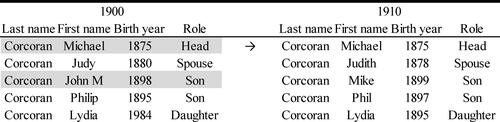
One of the major challenges associated with the feasibility of any attempt at large scale record linkage is its considerable computational requirements. Therefore, blocking criteria to limit the universe of potential matches are typically implemented, possibly at the expense of the exclusion of de facto links through reporting and digitization errors in characteristics such as name and state or year of birth. The second step of our linking procedure exploits the high confidence links that were made in the first step, while at the same time relaxing restrictive blocking criteria. The links already obtained provide valuable and specific information regarding where to look for individuals in the immediate circle of the person who was successfully linked in Step I. More specifically, consider a situation like that in Figure 3 below, where Michael Corcoran and his son, John M Corcoran (both highlighted in grey) are among the individuals who we attempt to link in Step I. In this hypothetical yet hardly unusual example, we were unsuccessful in linking the son, likely because his first name in 1910 is listed as Mike rather than John M. Also likely are situations where the year of birth reported in the 1910 census fails to be within the +/-3-year interval or where there is a change in the individual’s state of birth.

Figure 3. Using confirmed individual links to define universe of potential matches for Step II.

The logic of the second step is to use the 1910 household identifier as the primary blocking criteria when creating the universe of potential matches for all remaining (unlinked) family members. Since this restricts the population of potential matches (and thus also the computational requirements) to such a great extent, we are able to relax all other blocking criteria, including place of birth, year of birth, sex, and name similarity score. In fact, the only remaining blocking criterion is year of birth, however broadened to be an interval of +/- 10 years. Our training data consists of the remaining household members of the 1900 census individuals who we successfully hand linked in our training data for Step I. We linked these 3,776 individuals from the 1900 census to all individuals in the 1910 household to which we had linked the Step I training data individual – conditional on the year of birth blocking criteria. As a result of the household being the primary blocking criterion, the 1900 individual is on average only linked to 2.7 potential matches from the 1910 census. The resulting training data set, where we were able to manually link 61.4 percent of the 1900 census individuals (2,320 individuals), thus contains 10,101 observations.

Linking variables

Similar to the earlier outlined procedure, the algorithm in Step II is trained using characteristics such a Jaro-Winkler first and last name similarity scores, whether the race and place of birth of the 1910 potential match lines up with the 1900 census individual, and similarity in year of birth. Overall, however, a much more succinct set of linking variables are used, also reflecting the greater ease for the algorithm to confidently declare matches when the universe of potential matches is limited to the household.

While the incorrect enumeration or digitization of the individual’s sex remains an unusual phenomenon in the data, it nevertheless does occur. In fact, in the 1900 census, there are over 100,000 people who have a gender that doesn’t match their relationship to the household head, such as a daughter who is listed as male. As a consequence, a variable indicating whether the reported sex of the 1900 individual and the 1910 potential match is the same was created, naturally with the expectation that a mismatch on this characteristic will lower the predicted probability for any potential match. As indicated earlier, a more common occurrence is that the recorded name(s) of an individual change over time, for example from John M in 1900 to Mike in 1910. In order to capture this possibility, categorical variables measure whether the first and middle name initials in 1900, respectively, matches the first or middle name initial of the 1910 potential match. As a consequence, for the John M to Mike potential match, the variable intends to signal the presence of evidence in favor of a link, whereas this would not be the case for the John M to Phil combination of records.

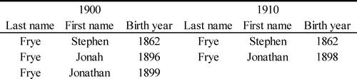
The two last linking characteristics we operationalize capture the individual’s role within the household as well as the presence of potentially competing matches. Firstly, we believe that the individual’s position within the household is characterized by varying degrees of volatility. More specifically, whereas a household head or spouse is likely to find themselves in a similar household a decade later, this is substantially less likely to be the case for a lodger or for a teenage child. Net of this, we believe that a 1900 individual and a 1910 potential match who occupy the same position within the household is a signal promoting a match. Lastly, we model the likelihood of incorrectly declaring a link by capturing the highest Jaro-Winkler score of a competing match in the household. The logic is perhaps most easily understood through an example like that displayed in Figure 4 below. In this situation, assume that we successfully linked the father, Stephen Frye, across the censuses and now turn to linking the remaining family members. In this case, the older of the two sons, Jonah, died in the intercensal period. Due to the high name similarity score between Jonah and Jonathan (Jaro-Winkler = 0.925), it is not, however, unlikely that many algorithms would have linked both Jonah and Jonathan in 1900 to the same 1910 record. As a consequence, both links would have been removed in the post-processing phase, as they represent duplicate matches. In an attempt to avoid this loss of data, for each 1900 individual, we obtain the highest name similarity score between the 1910 potential match in question and the remaining 1900 household members of that individual. In this case, for the Jonah 1900 record, while the name similarity score of Jonah and Jonathan (the 1910 potential match) amounts to 0.925, the corresponding value on the variable capturing the name similarity score of the most likely competing match amounts to 1. Consequently, the higher the latter score, the more likely it is that the potential match actually is another individual in the same household.

Figure 4. Operationalization of competing household match variable.

Training and implementing the algorithm

The procedure used to calibrate the linking algorithm for the Step II is the same as for Step I. Again, we opt for a logistic regression model when we calibrate the algorithm as well as which thresholds to use to optimize performance, performing ten loops over relevant threshold values to obtain stability. The estimated model parameters, along with variable means, are presented in Table A2, Appendix, corresponding to a precision of 96.2% and a recall of 97.0% at a maximum MCC value of 0.96.⁹

Table 2. Accuracy, by method.

	Step I	Feigenbaum	ABE
Confirmed links	46,342	28,404	26,459
Agreement rate with Family Tree database	97.7	86.5	93.4
Identical links declared by both algorithms		19,038	18,597
Only linked in Step I		98.5	99.0
		24,372	25,848
		97.0	96.5
Only linked by Feigenbaum/ABE		6,434	5,965
		18.9	62.2
Linked by both algorithms, different		2,932	1,897
Step I		95.0	90.7
Feigenbaum/ABE		0.4	5.4

Implementing the second step is considerably less computationally demanding due to the ability to block on household identifier. The approximately 46,000 links from Step I yields 237,000 unlinked 1900 household members – both men and women – to be linked to the 1910 census in Step II. Despite the substantial number of individuals that we aim to link, the fact that the 1910 universe of potential matches is limited to household(s) that their relatives belonging to the already confirmed matches have been linked to limits the number of potential matches. Consequently, if a given linked individual from a 1900 household where two members have been linked to different 1910 households in Step I, both these households will represent the universe of potential matches. Applying the parameter estimates and calibrated thresholds to the universe of potential matches, we obtain 104,932 matched men and women from Step II, for an accumulated total of linked men and women across both steps, amounting to 151,274 individuals.

Performance comparison

The linking procedure in this paper introduces two main innovations to automated record linkage: namely the algorithm’s systematic use of a more extensive set of characteristics as well as implementing a two-step procedure where we are able to leverage the existence of confident links to substantially relax typically used blocking criteria and thereby allowing for previously undiscoverable links to be found. It is, however, unclear how this approach performs compared to other methods of record linkage that are commonly encountered in the social scientific literature. We therefore proceed to implement both the Feigenbaum (2016) probabilistic record linkage method as well as the Abramitzky-Boustan-Erikson (2014) method (ABE¹⁰), in order to see how they compare. We will limit the comparison to the links obtained in Step I, by applying aforementioned methods in linking the same 100,000 men, comparing how the linked populations compare in terms of i) linkage rates, ii) precision, and iii) representivity.

When implementing the method proposed by Feigenbaum (2016), we use the same training data from Step I of the approach proposed in this paper.¹¹ In order to replicate the method in question as closely as possible to the original, however, we calibrate the performance thresholds using a probit estimator and with the same linking variables as Feigenbaum uses. Again, we select the α and β thresholds yielding the optimized performance based on MCC.¹² The ABE algorithm was implemented using the script provided by the authors,¹³ using first name, last name, and birth place as the exact match variables. Year of birth information is also used, first looking for exact matches, subsequently expanding the search to individuals with up to a two-year difference. NYSIIS standard names were also used to compare among potential matches.

Linkage rate

Table 1 illustrates the number of individuals out of the sample population of 100,000 men that were confidently linked across the methods evaluated in this paper. Beginning with Step I of our method, 46,342 men, or 46.3 percent, are linked across the censuses. The Feigenbaum and ABE linking methods yield a substantially lower number of confirmed links, with the ABE method yielding 26,500 links and the Feigenbaum method yielding 28,400 links.

While the methods confidently link differing shares of the sample population, another relevant aspect pertains to the degree to which the methods – when both declare a match – come to the same conclusion. The agreement rate is thus calculated conditionally on both compared methods declaring a link for a given 1900 census individual, reflecting the share of instances when they link to the same 1910 record. Across methods, the agreement rate is high, from 87 percent when comparing our method to Feigenbaum to 93 percent when comparing ABE with Feigenbaum.

Link accuracy

Despite the algorithms, to a large extent, being in agreement when declaring a match, a further investigation into how they perform when disagreeing will help to further understand the advantages and disadvantages associated with selecting one approach over another. A frequently relied upon measurement, precision, is not independent of the process as it is directly derived from the training data used to calibrate the linking algorithm. Instead, we make use of an extensive set of links from the Family Tree at familysearch.org. This comparison data is described in more detail in Price et al. (2021) and consists of pairs of records that have been attached to individual profiles on a genealogical website. This thereby provides us with an excellent and unbiased way to investigate the accuracy of our declared links, as the assessment is independent of all methods that are being compared. It, however, needs to be emphasized that while the database used contains a very large number of high confidence links that we can use to double check our declared links against, it does not cover the entire population. For example, out of the 1900 individuals who were successfully linked using Step I of our linking procedure, about 5% are covered by the database used to crosscheck performance. As a result, precision estimates are based on the subset of individuals in the 1900 census who are successfully linked by each method that overlap with the Family Search database.¹⁴

Table 2 illustrates that all methods similarly produce links that are of high quality in terms of agreement with the Family Search database. Among sample individuals from the 1900 census that are present and linked to a 1910 census record in the Family Search database, the accuracy across the three models range between a low of 87% (13% of declared matches do not agree with the Family Search database) for the Feigenbaum method to a high of 98% for the method described in this paper. Thus, despite linking a substantially higher proportion of the original sample of 100,000 randomly selected males from the 1900 full count census, the procedure outlined in this paper is able achieve a higher overall accuracy than both of the other algorithms.

Delving a bit deeper into what is behind the overall accuracy statistic unsurprisingly reveals a further increase when two compared algorithms are in agreement regarding the declared link. More specifically, when our algorithm declares the same link as either the Feigenbaum or ABE method, the Family Search database suggests an accuracy of 99 percent. Arguably of greater interest is the extent to which declared matches are correct across the methods when they arrive at different conclusions. Beginning with matches only declared by our algorithm, also representing the single most common category, the agreement with the Family Search database is only about a percentage point lower. In contrast, the decline in the agreement rate when examining matches only made by the Feigenbaum or the ABE algorithm is quite significant. More specifically, only in about 20 and 60 percent of the cases, respectively, does the match correspond with that in the Family Search database. Lastly, and further evidence to support our method’s improved ability to accurately distinguish between potential matches, in the cases where both our and the Feigenbaum or ABE algorithm declares a match for a 1900 individual but disagrees on which 1910 individual represents the true match, at least 90 percent of such cases result in our link corresponding to the Family Search database.

Representivity

The evidence we have presented suggests that the method introduced in this paper performs better than the other evaluated methods, with respect to both accuracy and linkage rate. A nontrivial consideration is, however, to what extent a linked sample resulting from any method of automated record linkage is able to reflect the underlying 1910 populations, as strong selection mechanisms in the process of record linking may result in linked samples that are not representative of the population of interest. As far as the method outlined in this paper is concerned, this is may be a particularly relevant concern since the household level features used to conduct linking may disproportionately link individuals experiencing household level and geographical stability over time. In order to investigate to what extent this appears to be the case, Table 3 presents each linked sample composition according to a range of characteristics, comparing them to a random subsample extracted from the 1910 full-count census, evaluating differences in means through t-tests. The comparison population is restricted to men, as well as to individuals 7 year of age and older and – if foreign born – with a time of arrival no later than 1900, serving to restrict the comparison population to individuals who were credibly present in the 1900 sample population, given the blocking criteria imposed.

Table 3. Representivity, by method.

	Census	Step I	Feigenbaum	ABE
Age	31.57	33.06***	35.29***	32.71***
7–20	0.33	0.33	0.28***	0.32***
21–45	0.44	0.41***	0.43**	0.44
46–60	0.15	0.17***	0.17***	0.15
61+	0.07	0.09***	0.12***	0.09***
Race
White	0.88	0.93***	0.93***	0.92***
Black	0.11	0.07***	0.07***	0.08***
Other	0.01	0.00***	0.00***	0.00***
U.S. born	0.87	0.89***	0.90***	0.90***
Household size	6.02	5.85***	5.74***	5.85***
1	0.03	0.01***	0.03***	0.02***
2–3	0.21	0.20**	0.23***	0.22***
4–6	0.42	0.44***	0.43***	0.43***
7–10	0.27	0.29***	0.26***	0.27**
11+	0.07	0.05***	0.06***	0.06***
Resides with spouse	0.43	0.47***	0.50***	0.46***
Resides with parent(s)	0.39	0.45***	0.37***	0.41***
Married	0.46	0.48***	0.51***	0.48***
Socioeconomic index^a	23.46	24.07***	24.58***	23.89**
1–9	0.14	0.12***	0.12***	0.13***
10–14	0.19	0.21***	0.22***	0.20***
15–25	0.14	0.15***	0.14	0.15**
26+	0.17	0.18***	0.19***	0.18***
Missing	0.36	0.34***	0.33***	0.34***
Resides in rural area	0.57	0.59***	0.59***	0.58***
Lifetime migrant (only for U.S. born)	0.26	0.21***	0.27*	0.25***
Region of residence
New England	0.07	0.08***	0.09***	0.08***
Mid-Atlantic	0.19	0.19	0.15***	0.18***
East North Central	0.20	0.23***	0.21***	0.22***
West North Central	0.13	0.15***	0.15***	0.15***
South Atlantic	0.13	0.12***	0.14	0.12***
East South Central	0.09	0.09*	0.09***	0.08***
West South Central	0.10	0.08***	0.09***	0.09***
Mountain	0.03	0.02***	0.03*	0.03
Pacific	0.05	0.04***	0.05*	0.05*
Observations	100,000	46,342	28,404	26,459

a Mean SEI score only calcucated for individuals with non-missing values

*** p < 0.01.

** p < 0.05.

* p < 0.1.

The linked populations resulting from all tested methods diverge from the comparison population across virtually all examined characteristics. Across all three linking methods, the resulting 1910 populations are older, more likely to be white, U.S. born and residing in a rural area, in addition to being characterized by a higher socioeconomic status than the comparison sample population. However, this is generally consistent with Bailey et al. (2020), who, in their evaluation of several of the most commonly used automated record linkage methods, note that “no algorithm (...) consistently produces representative samples”. Of potentially greater importance are differences across methods in their (in)ability to generate linked populations reflecting certain 1910 population characteristics. As far as our method is concerned, Table 3 reveals that the Step 1 linked population contains an overrepresentation of individuals residing with parents as well as a share of lifetime migrants that is lower than in the 1910 population that it should reflect. Should one wish to analyze a population that more closely resembles the comparison 1910 population, the data thus suggests both the Feigenbaum and the ABE method as offering a better ability to do so. There are, however, important implications linked to differences across methods’ accuracy, since we know that links generated by the Feigenbaum/ABE methods only are associated with considerably more noise, through incorrect links. The issue is further illustrated by Table 4, showing differences in means across the linking methods depending on whether observations were labeled as accurate links by the Family Search database. Beginning with our method, there are few statistically significant difference in means between the two categories, suggesting that – for example – the proportion of incorrect links among the foreign born does not differ from the proportion among the native born.

Table 4. Accuracy across methods, by 1910 characteristic.

	Step I		Feigenbaum		ABE
	Status of link compared with FamilySearch database
	Agree	Disagree	Agree	Disagree	Agree	Disagree
Age	35.40	33.52	35.19	37.95***	34.14	37.00**
Race
White	1.00	0.99	0.99	0.94***	1.00	0.91***
Black	0.00	0.01	0.01	0.06***	0.00	0.09***
Other	0.00	0.00	0.00	0.00	0.00	0.00
U.S. born	0.94	0.95	0.95	0.94	0.95	0.91**
Household size	6.19	5.93	6.14	5.87	6.16	6.47
Resides with spouse	0.59	0.60	0.57	0.58	0.55	0.52
Resides with parent(s)	0.42	0.37	0.42	0.27***	0.45	0.28***
Married	0.60	0.63	0.58	0.60	0.56	0.56
Socioeconomic index
1–9	0.09	0.12	0.09	0.14***	0.09	0.18***
10–14	0.30	0.30	0.29	0.27	0.27	0.25
15–25	0.14	0.12	0.14	0.13	0.15	0.12
26+	0.16	0.12	0.15	0.18	0.15	0.15
Missing	0.31	0.35	0.33	0.28**	0.33	0.29
Resides in rural area	0.70	0.70	0.70	0.63***	0.69	0.61**
Lifetime migrant (only for U.S. born)	0.27	0.27	0.27	0.37***	0.26	0.40***
Region of residence
New England	0.08	0.04	0.09	0.07	0.09	0.04***
Mid-Atlantic	0.14	0.12	0.11	0.14*	0.12	0.15
East North Central	0.28	0.21*	0.28	0.17***	0.28	0.23*
West North Central	0.18	0.17	0.19	0.16	0.19	0.16
South Atlantic	0.10	0.15	0.10	0.17***	0.09	0.14**
East South Central	0.08	0.08	0.07	0.10**	0.07	0.08
West South Central	0.07	0.07	0.07	0.08	0.06	0.08
Mountain	0.04	0.09*	0.05	0.04	0.04	0.07
Pacific	0.05	0.07	0.05	0.06	0.05	0.05
Observations in Family Tree database	4,804	113	2,599	406	2,752	195

*** p < 0.01.

** p < 0.05.

* p < 0.1.

Turning to remaining methods, important differences between the characteristics of correctly and incorrectly linked individuals emerge. More specifically, for both the Feigenbaum and the ABE methods, incorrect links are disproportionately found among individuals who are black, of low socioeconomic status, living in an urban area, and are lifetime migrants. Consequently, while these methods yield populations that in some respects more closely resemble the comparison 1910 population, our evidence suggests that this comes at the price of higher errors in the linkage of individuals possessing these very characteristics.

Step II links

Thus far, only the first step of our linking procedure has been evaluated, as it is only this that can directly be compared to the Feigenbaum and ABE linking methods. We now proceed to evaluate the complete set of links generated by the approach introduced in this paper. As previously reported, Step II links include remaining household members of individuals who were successfully linked in Step I; the Step II links benefit from the more narrowly-defined universe of potential matches. Additionally, while we restricted the population linked in Step I to men, we are here able to link a large population of women, primarily children and spouses. Table 5 illustrates that the additional approximately 105,000 individuals that are linked in Step II are characterized by a similarly high agreement rate compared to the Family Search database as in Step I, amounting to 98 percent.

Table 5. Accuracy, Step I and Step II.

	Step I	Step II	Total
Confirmed links	46,342	104,932	151,274
Agreement rate with Famiy Tree database	97.7	98.0	97.9

While Step I was developed to offer an alternative to already existing methods for linking historical records, the addition of Step II was primarily developed to be a tool useful for efforts to link complete-count populations or for research questions focusing on the household as a unit of analysis. More specifically, through the ability to isolate the universe of potential matches to such a great extent allows for the confident identification of links even when there is nontrivial discrepancy of traditionally used blocking criteria, such as place or year of birth. Resulting from the exercise of this paper, Step II yields an additional population of 59,000 women and 46,000 men. Table 6 presents the male (Step I + II) and female (Step II) populations compared to a randomly selected population of 500,000 individuals from the 1910 census. Focusing initially on men, the added population from Step II makes the linked population slightly younger and from larger households than the 1910 comparison population. In addition, the proportion of the population that resides with parents increases further. For women, selection according to the investigated characteristics generally resemble those for men, with the linked population disproportionately being white, not being a lifetime migrant, residing with a family member and in a larger household than the average woman from the 1910 census.

Table 6. Representivity, Step I and Step II combined by sex.

	Men		Women
	Census	Step I + II	Census	Step II
Age in 1910	31.76	30.85***	31.19	32.42***
7–20	0.33	0.41***	0.34	0.37***
21–45	0.44	0.35***	0.44	0.38***
46–60	0.15	0.17***	0.14	0.19***
61+	0.08	0.07***	0.08	0.06***
Race
White	0.89	0.94***	0.88	0.94***
Black	0.11	0.06***	0.11	0.06***
Other	0.01	0.00***	0.00	0.00***
U.S. born	0.87	0.89***	0.89	0.87***
Household size	6.00	6.55***	5.72	6.71***
1	0.04	0.01***	0.02	0.00***
2–3	0.21	0.12***	0.23	0.10***
4–6	0.42	0.41	0.43	0.41***
7–10	0.27	0.38***	0.26	0.41***
11+	0.07	0.08***	0.06	0.08***
Resides with spouse	0.43	0.39***	0.45	0.47***
Resides with parent(s)	0.39	0.56***	0.39	0.49***
Married	0.46	0.40***	0.47	0.48***
Socioeconomic index^a	23.41	23.27	25.03	29.23***
1–9	0.14	0.11***	0.04	0.02***
10–14	0.19	0.19***	0.02	0.01***
15–25	0.14	0.17***	0.07	0.07***
26+	0.17	0.16***	0.05	0.05***
Missing	0.36	0.37	0.81	0.85***
Resides in rural area	0.56	0.59***	0.54	0.57***
Lifetime migrant (only for U.S. born)	0.26	0.19***	0.24	0.20***
Region of residence
New England	0.07	0.08***	0.07	0.08***
Mid-Atlantic	0.19	0.19**	0.20	0.20**
East North Central	0.20	0.23***	0.20	0.24***
West North Central	0.13	0.16***	0.13	0.16***
South Atlantic	0.13	0.12***	0.14	0.11***
East South Central	0.09	0.09***	0.09	0.08***
West South Central	0.10	0.08***	0.09	0.07***
Mountain	0.03	0.02***	0.03	0.02***
Pacific	0.05	0.04***	0.04	0.03***
Observations	255,334	92,335	244,666	58,939

a Mean SEI score only calcucated for individuals with non-missing values.

*** p < 0.01.

** p < 0.05.

* p < 0.1.

Conclusions

A large empirical literature has emerged from numerous efforts to link individuals across historical records using various forms of deterministic and probabilistic machine learning techniques. We argue that the use of an expanded set of characteristics throughout the linking process yields higher precision and linkage rates, despite potential shortcomings in terms of stronger selection mechanisms. In particular, we propose the systematic use of information on household members and available contextual characteristics, both to maximize precision and to increase the ability to declare matches. We find that not only does our method yield a considerably higher number of links, but also does so with a higher degree of accuracy than two alternative methods. At the same time, it needs to be underlined that our method does yield a population with a larger underrepresentation of lifetime migrants, an important concern. It is also true, however, that there appears to be disproportionately more false links made by the ABE and Feigenbaum methods among the groups that are known to be more difficult to link, including lifetime migrants and non-whites. The consequences of sample selection as well as differing rates of linking errors by subgroups for substantive research questions are important and need to be explored in greater detail in future research.

The approach used in this paper is part of the process of eventually creating a longitudinal panel dataset that includes everyone who lived in the United States between 1850 and 1940 within the Multigenerational Longitudinal Project. Consequently, the method is straightforwardly modifiable to link censuses besides 1900–1910 either by using the same training data or after generating data uniquely suited for the censuses in question. Our method achieves very high match rates and precision, but it is likely that future access to additional records (such as birth, marriage, death, and administrative records) will make it possible to achieve even higher match rates. Efforts like the Longitudinal, Intergenerational Family Electronic Micro-Database (Bailey 2018) or the Census Longitudinal Infrastructure Project (Massey et al. 2018) point in the direction of using multiple records to link censuses. In addition, it is likely that combining machine learning with traditional genealogical approaches to linking records could identify linkages that are simply impossible to find using only one tool or the other (Price et al. 2021). Limiting linking approaches to immutable characteristics is likely to come at the cost of blocking or capping the match rates that are possible and increasing the number of false positives that are used to answer research questions.

Linkage strategies based on immutable characteristics that have dominated the literature for the past two decades highlighted the potential for selection bias in record linkage, and such linked datasets may still be preferred for some research questions. The approach in this paper is complementary and has its own set of advantages. Modern access to the full-count census records and fast computing make it possible for researchers to test the conclusions of their analysis to both types of linked samples. In addition, the tradeoff between the two approaches will only be present in the short run while the linkages of people across census records remains incomplete. It is likely combining multiple methods will allow the state of art to move more quickly to the eventual goal of linking the great majority of the population across all of the US census records, at which point concerns about selection bias will be reduced.

The algorithm presented in this paper is mainly based linking a small subsample of the underlying population from the 1900 full-count census to records from the 1910 census. The linking algorithm, available for download at ipums.org., was developed using the statistical software Stata (MP, version 14) and shares other methods’ challenges when it comes to scaling up the populations that one wishes to link. Unsurprisingly, the multitude of linking features employed by our method implies that the running time as well as the storage space and memory required exceeds that of the ABE and Feigenbaum methods in particular due to the latter’s relative simplicity. In order to overcome these performance issues, hlink has been developed within the Multigenerational Longitudinal Panel project. hlink uses a distributed processing engine to spread the workload across a cluster of computers, increasing the efficiency and the speed with which linking can be performed. As an example, linking the full 1900 population to the 1910 full-count census, yielding 30 million confirmed links, required a running time of 65 hours. The program, built on top of Apache Spark, will be released in the near future and is designed to allow the user to tailor the procedure outlined in this paper for other datasets, choosing which linking variables to include or exclude, as well as employing various linking methodologies, thereby further pushing the frontier of record linkage of individual level data. Through the implementation of the linking algorithm in hlink, we released the first public-use linked microdata for the 1900-1910, 1910-1920, 1920-1930 and 1930-1940 censuses in 2020 on the IPUMS website (https://usa.ipums.org/usa/mlp.shtml). The resulting datasets represent the largest populations to date that have been linked across each decennial pair of censuses. These linkages have consistently high overall accuracy, estimated at 97 percent or better across the datasets. Additionally, the representivity of the linked datasets largely resemble the figures presented in this article.

Acknowledgments

The authors acknowledge Ancestry.com for providing the underlying data making this research possible. The authors also gratefully acknowledge support from the National Institute on Aging (R01AG057679) and from the Minnesota Population Center (P2C HD041023) funded through a grant from the Eunice Kennedy Shriver National Institute for Child Health and Human Development (NICHD). We thank the editor, anonymous reviewers and participants at the 2019 Economic History conference on record linkage at Northwestern University ffor helpful comments and suggestions. We are also grateful for feedback from Ran Abramitzky, Leah Boustan and James Feigenbaum, as well as to Megan Moland, Jacob Van Leeuwen, Daniel Sabey and Tom Bryan for their excellent research assistance.

Disclosure statement

No conflicts of interest to report

Data availability statement

Data and syntax are to be published on ipums.org

Additional information

Funding

This work was funded by the research project “A Multigenerational Longitudinal Panel for Aging Research” (NIH/NIA, R01AG057679). Financial support from the Minnesota Population Center is also acknowledged, through core funding (P2C HD041023) from the Eunice Kennedy Shriver National Institute for Child Health and Human Development (NICHD).

Notes

1 A single individual typically provided information for all individuals in the household. While for the husband or wife of a small family with no unrelated household members, this task may not have been very complicated, this challenge would have been considerably more daunting for a servant or lodger (Magnuson 1995, 34).

2 The 1940 census, for example, only collected information on an individual’s parents respective place of birth for a small subsample.

3 The adjustment of the bigrams is through the first letter of the name being its own token. For example, Helgertz is split into “H”, “He”, “el”, “lg”, “ge”, “er”, “rt”, “tz”. Consequently, net of the Jaro-Winkler score similarity, the last names Helgertz and Wellington would pass this criteria, through “el”. Within the linking software developed to implement the algorithm outlined in this article, the use of first and last name adjusted bigrams reduces the baseline number of computations required during the generation of the universe of potential matches by 87 percent on sample datasets, reducing the runtime by about 70 percent (Wellington 201834).

4 In addition, an update of the 1910 full-count census resulted in a slight further reduction (n = 29) in the number of 1900 individuals, due to an adjusted year of birth variable.

5 Street names are cleaned, removing universal components, including “street”, “avenue”, “road” and “alley”.

6 In practice, however, the use of the 0.95 threshold rather than a 0.9 threshold, as used when identifying common household members, makes no practical difference for the performance of the algorithm.

7 The range of threshold values for α and β were 0.02-1 and 1-3, respectively.

8 This is obtained using a value ofα of 0.26 and a β of 1.

9 Values used for α and β are 0.41 and 1.1, respectively.

10 NYSIIS standard method.

11 Parameter estimates are presented in Table A3, Appendix.

12 The α and β values used were 0.08 and 1.7, resulting in an optimum MCC of 0.72. We suspect the training data used by Feigenbaum (2016) is characterized by a higher linkage rate than ours, despite the data that is linked being recorded 25 years apart. We believe our generally less impressive precision and recall values when calibrating our algorithm is linked to this difference in the training data.

13 https://ranabr.people.stanford.edu/sites/g/files/sbiybj5391/f/abe_basic_approach_1.pdf

14 Manual precision checks of all categories of cases presented in Table 3 but not covered by the Family Search database are provided in the Appendix, Table A4. While the manual check consistently suggests lower accuracy than the numbers provided by the Family Search database, a large internal consistency between the performance of respective linking algorithm remains.

References

- Abramitzky, R., L. Boustan, and K. Eriksson. 2014. A nation of immigrants: Assimilation and economic outcomes in the age of mass migration. The Journal of Political Economy 122 (3):467–506. doi: https://doi.org/10.1086/675805.
- Abramitzky, R., L. Boustan, K. Eriksson, J. Feigenbaum, and S. Perez. 2020. Automated linking of historical data. Journal of Economic Literature 59 (3):865–918.
- Abramitzky, R., L. P. Boustan, and K. Eriksson. 2012. Europe's tired, poor, huddled masses: Self-selection and economic outcomes in the age of mass migration. The American Economic Review 102 (5):1832–56. doi: https://doi.org/10.1257/aer.102.5.1832.
- Abramitzky, R., R. Mill, and S. Pérez. 2020. Linking individuals across historical sources: A fully automated approach. Historical Methods: A Journal of Quantitative and Interdisciplinary History 53 (2):94–111. doi: https://doi.org/10.1080/01615440.2018.1543034.
- Alexander, R., and Z. Ward. 2018. Age at arrival and assimilation during the age of mass migration. The Journal of Economic History 78 (3):904–37. doi: https://doi.org/10.1017/S0022050718000335.
- Antonie, L., K. Inwood, D. J. Lizotte, and J. A. Ross. 2014. Tracking people over time in 19th century Canada for longitudinal analysis. Machine Learning 95 (1):129–46. doi: https://doi.org/10.1007/s10994-013-5421-0.
- Antonie, L., K. Inwood, C. Minns, and F. Summerfield. 2020. Selection bias encountered in the systematic linking of historical census records. Social Science History 44 (3):555–70. doi: https://doi.org/10.1017/ssh.2020.15.
- Bailey, M. J. 2018. Creating LIFE-M: The longitudinal, intergenerational family electronic micro-database. University of Michigan Working Paper.
- Bailey, M. J., C. Cole, M. Henderson, and C. Massey. 2020. How well do automated methods perform in historical samples? Evidence from new ground truth. Journal of Economic Literature 58 (4):997–1044. doi: https://doi.org/10.1257/jel.20191526.
- Beach, B., J. Ferrie, M. Saavedra, and W. Troesken. 2016. Typhoid fever, water quality, and human capital formation. The Journal of Economic History 76 (1):41–75. doi: https://doi.org/10.1017/S0022050716000413.
- Blumin, S. M. 1976. The urban threshold: Growth and change in a nineteenth-century American community. Chicago: University Chicago Press.
- Chicco, D. 2017. Ten quick tips for machine learning in computational biology. BioData Mining 10:35. doi: https://doi.org/10.1186/s13040-017-0155-3.
- Collins, W., and M. Wanamaker. 2015. The great migration in Black and White: New evidence on the selection and sorting of southern migrants. The Journal of Economic History 75 (4):947–92. doi: https://doi.org/10.1017/S0022050715001527.
- Curti, M. 1959. The making of an American community: A case study of democracy in a frontier county. Stanford, CA: Stanford University Press.
- Dribe, M., B. Eriksson, and F. Scalone. 2019. Migration, marriage and social mobility: Women in Sweden 1880-1900. Explorations in Economic History 71:93–111. doi: https://doi.org/10.1016/j.eeh.2018.09.003.
- Eriksson, B. 2015. A link to the past: Linking and evaluating Swedish historical censuses. In Dynamic decades. A micro perspective on late nineteenth century Sweden, ed. by B. Eriksson (PhD Dissertation), 72, 111–47. Lund: Lund Studies in Economic History.
- Feigenbaum, J. J. 2016. Automated census record linking: A machine learning approach. Working Paper. https://scholar.harvard.edu/files/jfeigenbaum/files/feigenbaum-censuslink.pdf
- Ferrie, J. P. 1996. A new sample of Americans linked from the 1850 public use micro sample of the Federal Census of Population to the 1860 Federal Census manuscript. Historical Methods: A Journal of Quantitative and Interdisciplinary History 29 (4):141–56. doi: https://doi.org/10.1080/01615440.1996.10112735.
- Ferrie, J. P. 2005. History lessons: The end of American exceptionalism? Mobility in the United States since 1850. Journal of Economic Perspectives 19 (3):199–215. doi: https://doi.org/10.1257/089533005774357824.
- Fu, Z., P. Boot, P. Christen, and J. Zhou. 2014. Automatic record linkage of individuals and households in historical census data. International Journal of Humanities and Arts Computing 8 (2):204–25. doi: https://doi.org/10.3366/ijhac.2014.0130.
- Goeken, R., L. Huynh, T. A. Lenius, and R. Vick. 2011. New methods of census record linking. Historical Methods 44 (1):7–14. doi: https://doi.org/10.1080/01615440.2010.517152.
- Hopkins, R. 1968. Occupational and geographical mobility in Atlanta, 1870–1890. The Journal of Southern History 34 (2):200–13. doi: https://doi.org/10.2307/2204657.
- Knights, P. R. 1971. The plain people of Boston, 1830–1860: A study in city growth. New York: Oxford University Press.
- Magnuson, D. L. 1995. The making of a modern census: The United States census of population, 1790–1940. Ph.D. diss., University of Minnesota.
- Malin, J. C. 1935. The turnover of farm population in Kansas. The Kansas Historical Quarterly 4:164–87.
- Massey, C. G., K. R. Genadek, J. T. Alexander, T. K. Gardner, and A. O'Hara. 2018. Linking the 1940 U.S. Census with modern data. Historical Methods: A Journal of Quantitative and Interdisciplinary History 51 (4):246–257. doi: https://doi.org/10.1080/01615440.2018.1507772.
- Price, J., K. Buckles, J. Van Leeuwen, and I. Riley. 2021. Combining family history and machine learning to link historical records: The Census Tree data set. Explorations in Economic History, forthcoming.
- Rijpma, A., J. Cilliers, and J. Fourie. 2020. Record linkage in the Cape of Good Hope Panel. Historical Methods: A Journal of Quantitative and Interdisciplinary History 53 (2):112–29. doi: https://doi.org/10.1080/01615440.2018.1517030.
- Roberts, E., S. Ruggles, L. Dillon, Ó. Garðarsdóttir, J. Oldervoll, G. Thorvaldsen, and M. Woollard. 2003. The North Atlantic Population project: An overview. Historical Methods: A Journal of Quantitative and Interdisciplinary History 36 (2):80–8. doi: https://doi.org/10.1080/01615440309601217.
- Ruggles, S. 2002. Linking historical censuses: A new approach. History and Computing 14 (1–2):213–24. doi: https://doi.org/10.3366/hac.2002.14.1-2.213.
- Ruggles, S., C. Fitch, and E. Roberts. 2018. Historical census record linkage. Annual Review of Sociology 44:19–37. doi: https://doi.org/10.1146/annurev-soc-073117-041447.
- Thernstrom, S. 1964. Poverty and progress: Social mobility in a nineteenth century city. Cambridge: Harvard University Press.
- van den Berg, N., I. K. van Dijk, R. J. Mourits, E. Slagboom, A. A. P. O. Janssens, and K. Mandemakers. 2021. Families in comparison: An individual-level comparison of life-course and family reconstructions between population and vital event registers. Population Studies 75 (1):91–110. doi: https://doi.org/10.1080/00324728.2020.1718186.
- Wellington, J. 2018. HLink: An investigation into historical record linkage. Master’s thesis, University of Minnesota (mimeo).
- Wisselgren, M. J., S. Edvinsson, M. Berggren, and M. Larsson. 2014. Testing methods of record linkage on Swedish censuses. Historical Methods: A Journal of Quantitative and Interdisciplinary History 47 (3):138–51. doi: https://doi.org/10.1080/01615440.2014.913967.