Three new occupational status indices for England and Wales, 1800–1939

Abstract

Using 1.6 m marriages, 1837–1939, and a genealogy of 428,000 people 1600–2022, we estimate three new occupational status indices for England 1800–1939. The first, CCC-HISCO, re-estimates the HISCAM-GB index, using 30 times as much data. The second, CCC, uses the same association methodology behind HISCAM to assign status but employs richer occupation classifications than in HISCO-GB. The third, CCC2, links this richer set of occupations to measures of education and wealth, using principal component analysis. The close correlation between the CCC and CCC2 indices shows the HISCAM methodology generates occupational status indices, rather than just social proximity measures. All three new indices perform better than existing HISCAM indices, by the metric of father-son status correlation. They all imply less social mobility 1800–1939 than current indices.

Keywords:

• Occupational status indices
• association indices
• HISCAM
• social mobility
• intergenerational mobility

1. Introduction

Using a large new database of 1.6 million marriages 1837–1939, and a genealogy of 428,000 people 1600–2021, this paper estimates three new occupational status indices for England in the interval 1800–1939. The first of these, CCC-HISCO is a refinement of the HISCAM-GB index, but constructed using 30 times as much data as the original from marriage records 1837–1939.¹ The second, the CCC index, uses these same 1.6 million marriage records, and the same association method as HISCAM-GB, but with a richer set of occupational categories (462 versus 376). The third index, CCC2, again uses the richer set of occupational categories but combines instead six explicit measures of the social status associated with different occupations: specifically four measures of education and two of wealth.

We believe we have created improved social status indices for England 1800–1939 for the following reasons:

1. We have about 30 times as much data as was used to estimate the existing HISCAM indices, giving us much more precise estimates of the social status of occupations.²

2. We estimate directly a socio-economic status index based on education and wealth by occupation for the years 1800–1939 (CCC2). We use this to validate that the indices based on the association of occupations between fathers and sons, CCC and CCC-HISCO, correspond closely to socio-economic status.

3. In the CCC index by estimating status also for near 28,000 pairs with such status descriptors as Esquire, Gentleman, Landed Proprietor, Titled, Own Means, and Student we provide an index that better captures status for the upper tail of the status distribution.

4. Again in the CCC index, by expanding the occupational categories to 460, as opposed to the 376 occupational categories with status estimates in CCC-HISCO, we get a higher father-son correlation of status, which we argue below is the metric by which occupational status indices should be judged.³

We give online a CSV file with values for the CCC-HISCO index so that those with occupations classified using HISCO will have access to a better occupational status index for England 1800–1939. We do not know if the CCC-HISCO index will provide a better social status measure also for other countries in these years. That is an empirical question that will be determined by looking at the father-son correlations with CCC-HISCO versus other indices.

The creators of the HISCAM indices emphasize that these indices do not measure occupational social status, but instead are purely social interaction distance scales, and are not designed as proxies for the social prestige of occupations, or of income, or wealth.⁴ They measured only which occupations interacted in marriage and in families.⁵ However, in practice, the HISCAM indices have been widely used by researchers to measure socio-economic status. One recent paper noted, for example, “For Zeeland, we use the highest HISCAM SES (Lambert et al. 2013)… to measure socioeconomic status”(van Dijk, Janssens, and Smith 2019, 858).⁶

Further, a comparison of the three new indices developed here suggests that the association methodology does indeed also capture the social status of occupations. The explicit socio-economic status index, CCC2, is highly correlated with both the new association indices, with a correlation of 0.86 to the CCC index, and 0.82 to the CCC-HISCO index. The close correlation between the association indices and those that measure education and wealth provides a validation of the association methodology as also capturing occupational socio-economic status. The close correlation between the association indices and the socio-economic index just reflects the fact of social life that people associate in marriage and families with those close to them in socio-economic status.⁷

These three new indices all show that there was much less social mobility 1800–1939 than the current HISCAM indices imply. We argue that, in general, the measure of the quality of an occupational status index will be how high a correlation in father-son or father-in-law-son status the index produces. The first argument for this test of the quality of an index is that Goodman’s RCII association model which is used to produce the HISCAM and other indices sets occupational status scores to best predict the relative frequency of occupational pairings (Goodman 1979). But since the predicted frequency is higher the closer the rank scores of two occupations, this algorithm is also effectively maximizing the intergenerational correlation of occupational rankings. Since this is the criteria for the most predictive index, in comparing the quality of different indices it is consistent to use this as a benchmark for the quality of an index.

A second argument for using the father-son correlation as the test of quality of different indices is that there is evidence from a variety of sources that the true underlying correlation in social status between fathers and sons in England 1600–2022 is 0.75 or higher throughout this period (Clark 2023; Clark, Cummins, and Curtis 2022). Because any occupational index is imperfect, occupational status correlations will always be estimated as less than the true underlying correlation. A measure, however, of the quality of any index will be how close the estimated father-son correlation comes to the underlying intergenerational correlation.

Another argument for why the quality of an index is measured by the father-son correlation it produces is that if we take any existing index and make it worse by adding random noise to it, then it will lower the father-son correlation. If we estimate an index using just a small subsample of the available data, again we get a result with a lower father-son correlation. Thus the better an index captures true socio-economic status for occupations, the stronger will be the father-son correlation.

We also find good evidence in these new indices that occupational status is a continuum, best measured on a continuous scale as with CAMSIS and HISCAM. The popular alternative approach is to cluster occupations into a small number of discrete class categories, such as skilled manual workers, as was done for the UK by such as Robert Erikson and John Goldthorpe (Erikson and Goldthorpe 1992). This tradition was followed more recently by sociologists who deployed a seven-class system to measure social class in the UK in 2011 (Savage et al. 2013). However, such lumping of people into discrete social classes produces a poorer description of the movement of class across generations than does continuous measures of social status. This is illustrated in Figure 1, which shows the average social status of sons 1837–1879 on the CCC scale relative to the average status of fathers. There is a very strong linear relationship, with the same slope all along the status distribution. A straightforward regression to the mean dominates. There are no signs of any unusual persistence for upper or lower classes. The CAMSIS and HISCAM continuous measures of occupational status are a better approach than the alternative discrete class schemas.

2. The HISCAM indices

The standard indices to measure male intergenerational occupational status mobility before 1939 in Britain have been those from the HISCAM project. The HISCAM measures for Britain 1800–1938 were derived using data on pairs of occupations, mainly father-son or father-in-law-son pairings. An algorithm was employed to give rank scores to each occupation in a way that best predicted the observed relative frequency of occupational pairs.

Occupations for the HISCAM status scores were coded to a standardized international occupation classification system HISCO, which set out to have an internationally comparable set of occupation codes based on the 1,300 most common male and female occupations 1800–1938 in Belgium, England, France, Germany, Netherlands, Norway, Quebec, and Sweden.⁸ Because of the desire for a comparable international coding of occupations the occupational classifications are detailed. A weaver, for example, can be coded as Cloth Weaver (hand), Cloth Weaver (Machine, except Jacquard Loom), Cloth Weaver (Hand or Machine), Weaver (Specialization Unknown), or Other Weavers and Related Workers.

In HISCAM-GB there are only 376 occupational categories, out of a potential 1,300, with assigned scores. These assignments were based on 51,419 occupational pairings.⁹ Relative to the number of occupational categories used, the data is modest, so that for many of the less frequent occupational categories, the assigned status will be measured with significant error.

To rank occupations on a single rank scale CAMSIS and HISCAM used Goodman’s RCII association model (Goodman 1979).¹⁰ The resulting estimates for HISCAM are normalized to have mean of 50 and standard deviation of 15, then truncated to have a minimum value of 1 and a maximum of 99.

The alternative general HISCAM-U2 index has a much larger empirical base, 1.3 million occupation pairs, again composed almost equally of father-son and father-in-law-son occupational pairings. The number of pairings underlying the index is, in Belgium, 56,774, Britain, 51,419, France, 55,459, Germany, 12,301, Netherlands, 564,726, Quebec, 552,521, and Sweden, 31,219. Because of the small sample sizes for Germany and Sweden, the developers of HISCAM suggest for these countries, that using the universal scale may be preferable.

The HISCAM and CAMSIS indices have two modifications from the Goodman association model to address several common practical problems in estimating association models. The first is that of sparse categories. The fine grid of occupations, together with the modest numbers of occupational pairings means that many occupations appear infrequently. Where an occupational category has few individuals, the RCII estimator often will not converge to a stable set of occupational status rankings. HISCAM and CAMSIS address this by combining any occupation with fewer than 30 observations with other similar occupations.¹¹ But this, of course, introduces further error into the index.

The second problem are so-called diagonals and pseudo-diagonals. Diagonals are cases where each person in the pair has the same occupation. Pseudo-diagonals are cases where even though the occupations have different statuses, they are frequently found together in pairings. These would include particularly farmer and farm-worker which are found commonly both in husband-wife pairings and also father-son pairings.¹² To avoid the distortions in status rankings CAMSIS and HISCAM typically drop pairs of diagonals and pseudo-diagonals. The HISCAM project, however, concluded that dropping diagonals was insufficient, and dropped the agricultural sector from their analysis entirely. Farm jobs were assigned scores equal to the average of all occupations paired with farming occupations.

With the new data assembled below, we find that these two problems do not arise, and we can estimate association models without any restrictions. In particular, the small size of the farm sector in England by 1837 means that there are plenty of father-son and father-in-law-son pairings with one party in agriculture and the other outside farming with which to estimate the status of farming occupations. Table 1 shows for marriages 1837–1879, the numbers of pairings of farm occupations father-son with other farm occupations and with non-farm occupations. Thus, for example, while there are 28,843 father-son pairings where both are farmers, there are 50,511 pairings where one is a farmer and the other in a non-farm occupation.

Another occupation where there was relative isolation from other sectors of the economy was coal mining, where coal villages could have a workforce concentrated in mining. Here we might expect a complete dominance of father-son pairs who were both in coal mining, making it hard to estimate the social status of coal miners. However, while we do find in marriages 1837–1879, 27,050 father-son pairs who were both coal miners, we also find 30,082 pairs where only one in the pair was a coal miner. So even here there is plenty of connection between coal miners and other occupations to allow an estimate of the average social status of coal miners.

3. Three new occupational status indices, England and Wales, 1800–1939

Using two large new databases, in this paper we construct three new occupational status indices for men in England 1800–1939. The first of these indices is a refinement of the HISCAM-GB index for England, which we label CCC-HISCO. Here we estimate for 319 identified HISCO categories a new RCII index using occupational data for 2.36 million father-son and father-son-in-law pairs, from 1.6 million marriages 1837–1939. This new index is thus based on nearly 30 times as much data as the HISCAM-GB index.

This index also uses more father-son pairs than in the entire eight country HISCAM occupational database.¹³ We carry out the index estimation separately using the father-son occupation associations, and the father-in-law-son associations, and then take the average of these occupational rankings in forming the overall index.

Because of this much greater set of data, we are able to avoid the improvisations forced on the HISCAM creators by data limitations, such as amalgamating occupations in the estimation. Because of the close interconnections shown in Table 1 above between farm and non-farm occupations, we can estimate the model without having to drop and then approximate occupations in the agricultural sector. Lastly, we are able to implement the RCII model without dropping diagonal, or quasi-diagonal, observations. However, only 319 out of 1,300 potential HISCO occupations are matched to the occupation labels in our data.

The second of these new indices, CCC, is an association index, as with CAMSIS and HISCAM. We also employ an occupational scheme with a richer set of 462 occupational categories (as opposed to the 376 in HISCAM-GB). These categories were those that showed up most often in the nearly 5 million occupational titles that occur in our marriage database. In Appendix A, we list these occupational titles and the corresponding HISCO occupation numbers. We also included status titles that were not included in HISCO, such as Esquire, Gentleman, Landed Proprietor, Titled, Own Means, Student, and Pauper. In this case, the correlation between the RCII index created using fathers and sons versus the RCII index using fathers-in-law and sons is 0.80.

The third new index, CCC2, is constructed in part using a large genealogical database for England that has information on such outcomes as occupation, wealth at death, and educational status. It also employs data from the marriage records on groom literacy by occupation. This index is a much more direct estimate of average socio-economic status by occupation. Nicely, it is constructed completely independently of the information underlying the CCC index. It serves to validate that the CCC index is indeed capturing occupational status, rather than just social proximity.

Scholars use occupational status indices in part to measure the degree of occupational status inheritance, and also to measure the degree of occupational status assortment in marriage. It is thus potentially problematic to compare status inheritance and marital assortment over time when the indices to measure this are estimated by maximizing both of these correlations. The CCC2 occupational status index has one virtue in being completely independent from parent-child occupation correlations, and also from marital occupation correlations. This index has six components.¹⁴

1. Literacy rates by occupation, 1837–1879

2. Probate Rate by occupation, 1858–1939

3. Average log wealth at death by occupation, 1858–1939

4. Average attainment of higher education by occupation, 1800–1939

5. Proportion in schooling ages 12–18 by occupation, 1851–1939

6. Proportion at work ages 12–18 by occupation, 1851–1939

The literacy rate by occupation is estimated from 0.4 million observations of the signature literacy of grooms 1837–1879 and their occupations. The period 1837–1879 was used even though there is literacy data all the way to 1939 because after 1880 signature literacy rates for grooms are near 100% so that this measure contributes little information for 1880 and later. For marriages 1837–1879 only 64% of grooms could sign the register, so that this measure contributes significant information on educational status by occupation. This measure will discriminate more on the status of lower status occupation since almost all men in higher status occupations will be literate.

The second measure, the probate rate, shows the fraction of men by occupation that had some wealth at death, for deaths 1858 and later. The third measure is the average ln wealth at death, measured relative to average estimated ln wealth at death for each decade in England. For those not probated, wealth at death is taken as half the level of wealth at which probate was legally required in the year of death. These two wealth measures correlate highly. But the first better measures differences in wealth for occupations lower in the wealth distribution, while the second better measures wealth differences for higher status occupations.

The fourth measure is an indicator of what fraction of men by occupation attended university, or achieved an equivalent higher education, such as medical training in a teaching hospital, or membership of an engineering society, or qualification as a chartered accountant. This again is a measure which discriminates more for higher status occupations.

The final two measures are whether the person was observed in schooling, or at work, when recorded in a census or population register 1851–1939 ages 12–18.¹⁵

We construct a composite index of our six occupational status variables using Principal Components Analysis (PCA).¹⁶ PCA, originally created by Pearson (1901) and later developed by Hotelling (1933), is a widely used technique to simplify multidimensional data. PCA generates linear transformations of the six status measures into a set of new variables: uncorrelated principal components. By construction, the first principle component captures the greatest variation possible by any single linear transformation.

We use this first principal component as our unidimensional index of occupational status. The specific formula for the CCC2 index in this case is, $$\begin{array}{l}\mathit{\text{CCC}}2=\text{\hspace{0.17em}2}0.786\hspace{0.17em}+\text{\hspace{0.17em}2}0.388\mathit{\text{LITERACY}}+\\ \text{\hspace{0.17em}16}.959\mathit{\text{DPROB}}+\text{\hspace{0.17em}2}.685\mathit{\text{LNW}}+\text{\hspace{0.17em}18}.741\mathit{\text{DED}}-\\ \text{\hspace{0.17em}17}.351\mathit{\text{DWORK}}+\text{\hspace{0.17em}18}.344\mathit{\text{DSCHOOL}}\end{array}$$ where LITERACY is the average male literacy rate by occupation, DPROB is the fraction of men probated by occupation, LNW is the average ln wealth of men by occupation, DED is the average share achieving higher education, DWORK is the average share at work 12–18, DSCHOOL is the average share in school 12–18. Where one of the six measures was missing we estimated occupational status using the other five in the same fashion, or interpolated the missing values from similar status occupations.

4. Data

We use two sources of data to construct these new indices. The first is a set of 1.6 million marriage records in England 1837–1939 which were transcribed by volunteers to the FreeREG organization, and posted on their web page.¹⁷ The FreeREG marriage records, where the information comes from marriage record copies deposited in local record offices, all come from church weddings, and exclude civil marriages. But though civil marriage was introduced in England in 1837, such marriages remained a small minority of all weddings before 1914. In 1841 civil marriages were 1.7% of all marriages. In 1914, they were still only 24%, and even in 1952, 31% (Haskey 2015).

These marriage registers typically record whether the bride and groom were literate (through their ability to sign the marriage register). They also give occupations for the groom, his father, and his father-in-law.¹⁸ The data we have available by period is shown in Table 2. Because transcribing these marriage records is a volunteer effort based on local interests, the number of marriages recorded by county for the years 1837–1939 varies considerably by county. Four counties contain about 50% of the marriages transcribed for England: Kent, Lancashire, Lincolnshire, and Staffordshire. But these counties were very different in terms of occupations and urbanization so that the overall sample generated seems representative of England as a whole.

From the resulting database Marriages of England (MOE) we construct our CCC-HISCO and CCC index of male occupational status 1837–1939. We also construct from the literacy data for grooms 1837–1879, a measure of literacy by occupation.

In constructing the CCC index, and in estimating literacy by occupation we convert the more than 100,000 individual occupation description strings in these 1.6 million marriage records into 462 simplified occupations. The more than 2,000 different types of clerks listed, for example, were translated into Bank Clark, Civil Servant-Clerk, Clergy-Church of England, Commercial Clerk, Legal Clerk, and Parish Clerk. We also coded these occupations by their HISCO equivalent, and as noted constructed a new index CCC-HISCO using this occupational scheme.

Figure 2 shows the distribution of occupational status scores on the CCC index, on a 0–100 scale, across the whole population of grooms. The distribution is modestly skewed, with a median status of 42 out of 100. Where multiple occupations were given in the marital records we used the first listed, except in the case that the first was a military occupation. In that case, we coded the person to their civilian occupation.

The second source of data we have is a genealogical database 1600–2022 of 424,000 linked persons in rare surname lineages [Families of England (FOE)] where we can obtain for a subsample of men their wealth at death, their probate status, their educational status ages 12–18, and their attainment of higher educational qualifications.¹⁹ Table 3 shows the amount of data available for men by occupation from this source.

The schooling 12–18 variable is estimated from a set of census reports on whether a person in this age range was at work, in schooling, or an apprenticeship, or nothing was recorded. To allow for the cases with nothing recorded we take the raw measure of schooling as the average of an indicator variable for in schooling and one minus an indicator variable for at work. However, we correct this variable for the average age people were observed at in each occupation by regressing the fraction in schooling against average age and adjusting all the raw measures to a standard age of 15. This results in some cases in a negative estimate of the proportion of schooling on this adjusted measure. The two wealth measures are the fraction of men whose estates were probated at death by occupation, and the average ln wealth of those probated normalized by average wealth at death for all men by decade 1850–1939.

These six measures of educational and wealth status correlate reasonably well, as Table 4 shows. Though the quantity of data here is much smaller than for the marriage database, we shall see that it produces an index that is nearly as good in terms of intergenerational correlations as the family association index.

The principal component analysis decomposition works well with the six status indices we employ here. The first principal component accounts for 67% of the variance in the six status measures. We normalize the resulting CCC2 index to a scale of 0–100. Figure 2 also shows the distribution of the status values of the CCC2 index on this 0–100 scale, across the whole population of grooms. The distribution is asymmetrical, with the mass of men having occupations in the 20–50 occupational status range. But there is a long tail of upper status occupations in the 50–100 range. Table 5 shows the characteristics of the top 10 and bottom 10 occupations in the CCC2 ranking. The top and bottom occupations seem very plausible for those positions.

Table 6 shows the ranking of the top 10 occupations in the CCC index, and their comparable ranking in the CCC2 index.

Though the CCC and CCC2 indices were produced using entirely different methods, and completely different data, they show a 0.86 correlation in the status assigned to occupations. Figure 3, for example, shows the estimated status of the 462 occupations in the CCC index versus the CCC2 index. The graph also shows the most significant outliers. There is no obvious pattern to these. This shows that family association style status indices produce occupational status rankings that are very close to those implied using direct socio-economic measures, such as education and wealth. This is confirmation of the validity of the HISCAM approach also as a measure of the socio-economic status of occupations.

The CCC2 index also produces much higher intergenerational correlations in occupational status than the existing indices. Where we estimate, however, familial correlations using the marriages database we potentially run into the problem that the CCC index was constructed using the same data and with an algorithm based on maximizing the father-son correlations in occupational status. However, we can test whether this will be a significant source of bias by taking the marriage data, dividing it randomly into two halves, and then estimating the CCC index on the first part. We can take this 50% index and estimate the father-son and father-in-law-son correlations using both the training 50% of the data and the testing 50%. If these estimates do not differ significantly across the two sub-samples of the marriage data, then we are getting an unbiased estimate of intergenerational mobility even using the marriage sample and the RCII status index derived from that same sample.

Table 7 shows the results of this test. The evidence from the table is that there is no significant upward bias in intergenerational correlation estimates when we use an RCII status index derived from the same data with which we estimate the intergenerational correlation. Thus on either database, we can do a test of the quality of the different occupational indices.

In Appendix A.1, we give the CCC-HISCO scores, as well as the HISCAM-U2 and HISCAM-GB status scores, for the 319 HISCO occupations we are able to rank. In Appendix A.2, we give the status scores of each of the 462 FOE occupations on both the CCC and CCC2 indices.

5. Comparing the new indices with HISCAM

Table 8 shows the correlation in occupational status as measured with the three new indices CCC, CCC2, and CCC-HISCO compared to HISCAM-GB and HISCAM-U2. As can be seen, all these indices correlate strongly. Note in particular that the CCC2 index, which is constructed both in a different manner and using completely separate data, correlates well with all the association type indices.

However, the best index of occupational status will be the index which produces the highest correlations of son to father and groom to father-in-law. Table 9 shows these father-son correlations for all five indices 1837–1939. Though the CCC indices correlate well with the two HISCAM indices, all the CCC indices produce substantially greater father-son and father-in-law-son correlations than does either HISCAM-GB or HISCAM-U2. Thus on this criterion of fit, they are a better index of social status for England 1837–1939. The true correlation in status on the CCC index, for example, averages at 0.68 for these years, well above the 0.54 correlation found with HISCAM-GB.

Figures 4 and 5 show in detail how the individual occupations compare in estimated status between HISCAM-GB and CCC-HISCO, and HISCAM-U2 and CCC-HISCO. The ten occupations with the greatest sum of squared deviations in status are labeled by name. In general, the CCC-HISCO index shows much greater differences in status for occupations at the lower end of the status scale, such as coal miners and laborers, than do the HISCAM indices. Other than that, however, there is no particular pattern to the deviations across the indices.

The CCC2 index performs somewhat less well than the CCC index, as measured by intergenerational correlations. But it must be remembered that five of the six sub-indices that compose this index were created using sample sizes in the order of 10,000–50,000, as opposed to the 2.4 million observations used to construct the CCC and CCC-HISCO indices. If sample sizes for constructing the CCC2 index were substantially increased it might well correlate better across generations than the CCC index.

Table 9 also shows that on all these indices there appears to be an increase in social mobility rates from 1837 to 1939. For the CCC index, for example, the measured father-son intergenerational correlation falls from 0.71 in 1837–1859 to 0.60 in 1900–1939. On HISCAM-GB the fall is from 0.59 to 0.44.

However, the 0.68 intergenerational correlation recorded using the CCC index can be shown to be still well below the true correlation for 1837–1939. This is because of two forms of remaining error in the index. The first is the mismeasurement of the exact average status of each of the FOE 462 occupation categories. The second is that people whose occupation is assigned to the same of the 462 categories will often actually differ in occupational status. The category “clerk,” for example, covers occupations that differ widely in earnings, and in other measures of occupational status.

Suppose a person’s true occupational status is z. Suppose also their assigned status on an occupational index is Z. Then there will be two independent errors linking their assigned status to their true status. Z = z + u + e, where e is the error in measuring the true average occupational status of the assigned occupation Z. u is the error caused by the range of occupations that fall under the label Z, each with a different underlying status.

When we measure intergenerational mobility with such a social status index the estimate is biased downwards by a factor: (1) $$\frac{{\sigma }^2}{{\sigma }_z^2+{\sigma }_u^2+{\sigma }_e^2}$$(1)

For the CCC and CCC2 indices, because of their entirely independent construction, the error component e attached to errors in the average occupational status by category will be independent, but not the within-category component u. Assuming the error term e variance is the same for each index, the correlation between these indices 0.86 will be (2) $$\rho =\frac{{\sigma }_z^2+{\sigma }_u^2}{{\sigma }_z^2+{\sigma }_u^2+{\sigma }_e^2}=0.86$$(2)

This implies that the error component in these indices we have derived has to be at least 12% of the variance in measured status. It also implies that if we multiply our father-son correlations by 1.16 we will get an estimate closer, but still not as large as, the true underlying persistence of occupational status across generations. Since that correlation for the CCC index is 0.68, the true intergenerational correlation in occupational status has to be at least 0.78. When we add the attenuation caused by the variance within occupational categories, the true underlying correlation of occupational status in England 1837–1939 must be above 0.8. This is well above the 0.51–0.53 correlation reported for this period using the HISCAM-U2 and HISCAM-GB occupational status indices.

As noted above, the parish register data we relied upon to construct the CCC and CCC-HISCO indices was over-sampled in four counties—Kent, Lancashire, Lincolnshire, and Staffordshire—which together accounted for almost half the observations. Table 10 shows the estimated intergenerational correlation from each of these counties, as well as from the rest of the data. Are there significant geographic differences in intergenerational social mobility that might explain the much stronger intergenerational correlations found with the CCC and CCC-HISCO indices than for the HISCAM indices? As can be seen in Table 10, for three of the four counties there is no substantial difference in the intergenerational occupational status correlation and that for the rest of the country. Only for one county, Lancashire, do we observe a substantially different correlation compared with the rest of the country, and that is lower at 0.56 versus 0.68. If we were to reweight the data to be nationally representative, if anything we would likely observe the same or an even higher intergenerational occupational status correlation. Thus the particular geographic concentration of the marriage records does not in any way explain the very high intergenerational correlations we observe.

6. Conclusion

Using large quantities of new data, we construct three new independent occupational status indices for England in the years 1800–1939, the CCC, CCC2, and CCC-HISCO indices. These new indices all provide more accurate measures of the social status of occupations in these years than the existing HISCAM indices (HISCAM-GB and HISCAM-U2). Appendix A gives the estimated status for all occupations on these new indices.

Second, we validate that association indices of occupational status do successfully capture the socioeconomic rank of different occupations as measured by the educational and wealth status of the holders. The two new association indices, CCC and CCC-HISCO are both highly correlated with the third new index, CCC2, which was entirely constructed from six measures purely of socioeconomic status. Though some scholars continue to emphasize the difference between social interaction distance scales and social status scales, we show above that effectively such scales measure the same thing, the social status of occupations. Association indices thus are very good measures not just of social networks, but also of socio-economic status. An important contribution of this paper is thus to show that association indices do not capture a distinct feature of social life. Social interactions seem to be dominated by social status.

We also find that with sufficiently large sets of data, these association indices can be estimated for England without having to make the various adjustments and status assignments found in the HISCAM indices. Thus this paper is a strong validation of the strength of the association approach to constructing status indices and of the general validity of the indices so constructed.

Third, we show how dependent measures of intergenerational occupational status mobility are on the quality of occupational indices. The more accurate the status index the lower are measured rates of intergenerational mobility. While this shows that social mobility rates in England 1800–1939 were low, it also shows that all comparisons of intergenerational occupational mobility over time and place using such indices are suspect. The measurement errors embedded in occupational status indices depend on the quantity of data available to construct the index, the employment structure in the society in question, and the way occupations are described in different societies. Traditional comparisons of social mobility across time and place using such indices are therefore unreliable. We explore this issue in more depth in a related working paper and suggest a method of extracting the true underlying intergenerational correlations in status (Clark, Cummins, and Curtis 2022).

However, there are many purposes for which these imperfect indices are still highly useful. One example is that the popular conception that women tended to marry-up socially is not true for England 1837–1939. We can measure the social status of both bride and groom using the occupational status of their fathers. When we do this the status of the groom’s father, on average, equaled the status of the bride’s father throughout these years. Women were not marrying men whose family background, on average, showed higher social status (Clark and Cummins 2023).

The CCC-HISCO index is a higher quality index for England than HISCAM-GB or HISCAM-U2. It is likely that this index will also be of better quality than the HISCAM indices for Germany, Sweden, Belgium, and France given the much larger size of the dataset it is based upon. Potential users will be able to determine if it works better by comparing the resulting father-son or father-in-law-son-in-law correlations. For the convenience of users, we have provided a link to the CCC-HISCO scores.²⁰

Disclosure statement

No potential conflict of interest was reported by the author(s)

Additional information

Funding

The substantial data collection in this paper was made possible by the generous financial support for Economic History at UC Davis of Michael Dearing.

Notes

1 For details on the construction of the HISCAM-GB and HISCAM-U2 association indices see Lambert et al. (2013).

2 The source of the HISCAM-GB index, as without association indices, is a much smaller set of marital records 1837–1938 for England (Lambert et al. 2013).

3 A CSV file with the three new indices and the existing HISCO_GB and HISCO_U2 indices is available for download on the Harvard Dataverse https://doi.org/10.7910/DVN/0AZTNV.

4 https://www.camsis.stir.ac.uk/Data/Britain91.html. See Lambert et al. (2013) and Prandy and Lambert (2003).

5 http://www.camsis.stir.ac.uk/hiscam/. HISCAM is an empirical estimate of the average relative position within the structure of social stratification occupied by the incumbents of occupational unit groups based on patterns of intergenerational occupational connections.

6 See also, as examples using HISCAM scores as measures of social status, Bailey, Hatton, and Inwood (2016), Brea-Martínez and Pujadas-Mora (2018), Connor (2017, 2019), Cummins (2020), Debiasi and Dribe (2020), Dribe and Helgertz (2016), Dribe and Karlsson (2022), Dribe and Quaranta (2020), Fernihough (2017), Hällsten and Kolk (2023), Jaadla et al. (2020), Knigge (2016), Knigge et al. (2014), Knigge, Van Leeuwen, and Maas (2014), Lan and Longley (2021), Rosenbaum-Feldbrügge (2019), Van Leeuwen and Maas (2023), and Zhu (2022).

7 One referee was insistent, nonetheless, that “the sociological term ‘status’, when used in the context of measures of social stratification, is a different concept to that of ‘socio-economic status’.” We do not deny that there are other interpretations of status distinct from socio-economic status. All we claim here is that association status measures are highly correlated with socio-economic status. Thus those interested in socio-economic status can employ association index methods to construct measures of socio-economic status.

8 HISCO, or Historical ISCO, is a modification of the 1968 version of the International Standard Classification of Occupations (ISCO-68) (Van Leeuwen, Maas, and Miles 2004). http://historyofwork.iisg.nl/index.php.

9 Lambert et al. (2013), Table 1.

10 Hendrickx (2004) and Xie (1992, 2003) provide less theoretical introductions to the RCII model.

11 In the HISCAM indices estimated using only data from one country, when a category was small and its score varied substantially from the category’s score in the universal scale, its score was replaced by the average of the original score and the score in the universal scale.

12 In the intergenerational mobility literature, farmers are often a problem regardless of methodology. See, for example, Feigenbaum (2018), Xie and Killewald (2013), and Appendix IV of Abramitzky, Platt Boustan, and Eriksson (2012).

13 The HISCAM database has 1.2 m father-son occupational pairs, but 0.5 m of these come from Quebec, where the occupations are mostly in agriculture.

14 Using information from six components gives our measure an advantage over occupational status scores that rely just on income. Occupational income scores often overlook a lot of within-occupation variation; see, for example, Espín-Sánchez et al. (2019), Inwood, Minns, and Summer Eld (2019), and Saavedra and Twinam (2020). By adding the additional six series, we will capture a lot more variation within-occupation.

15 The censuses of 1851–1921 give such information, as does the population register of 1939.

16 Simple averaging would be inefficient as information would be lost by combining high variability measures, such as average wealth, with those with low variability such as education or literacy. PCA allows the data to tell us the weights that maximize variability, without reference to any target, or output, measure. In this way, PCA is a type of “unsupervised learning.”

17 We added to these records 21,339 marriages in Essex parishes 1837–1939 that we ourselves collected. Much less often in earlier years they give an occupation also for the bride.

18 See note 15 above.

19 This dataset is described in detail in Clark (2023) Supplementary Materials.

20 http://neilcummins.com/CCC-HISCO.csv.

Appendix A

A.1. Tabular summary of the CCC-HISCO index

Table A1 shows CCC-HISCO occupational status values in comparison with those of the HISCAM-U2 and HISCAM-GB index. The occupations are listed in order of the HISCO codes. A brief description of each occupation is given. This table is available online at http://neilcummins.com/CCC-HISCO.csv.

Table A1. CCC-HISCO, HISCAM-U2, and HISCAM-GB indices by HISCO.

HISCO	Description	CCC-HISCO	HISCAM-U2	HISCAM-GB
11010	Accountant, General	65.5	71.8	65.0
1110	Chemist, General	62.2	82.8	84.1
1200	Physicists	93.7	82.8	84.1
1210	Physicist, General	72.5	79.7	80.4
12110	Lawyer	89.2	99.0	75.5
12210	Judge	89.4	99.0	99.0
12410	Solicitor	83.7	99.0	75.5
13020	Teacher, Level, and Subject Unknown, Not University	55.7	67.5	58.1
13100	University and Higher Education Teachers	70.3	99.0	71.4
1330	Geological Scientist	74.3
13320	First-Level Education Teacher	54.1	65.6	64.2
1390	Other Physical Scientists	78.0
13940	Head Teacher	75.1	81.7	77.8
14120	Minister of Religion	83.8	99.0	74.2
15120	Author	53.1	76.2	71.9
15915	Journalist	63.4	91.2	71.9
16130	Painter, Artist	64.0	76.5	76.8
16200	Commercial Artists and Designers	56.2	66.1	59.8
16220	Commercial Artist	54.7	68.0	67.0
16310	Photographer, General	54.8	66.1	59.8
17140	Instrumentalist	49.1	59.0	57.6
17320	Actor	63.3	59.3	57.6
17420	Theatrical Producer	52.4	59.3	57.0
18020	Professional Sportsman	31.1	59.3	57.6
19120	Librarian	62.5	89.3	91.5
20110	Legislative Official	100.0	99.0	67.7
20210	Government Administrator	66.0	92.8	70.4
21110	General Manager	60.3	88.2	54.4
2120	Building Architect	71.2	85.4	66.0
21240	Contractor	46.3	68.8	67.9
21340	Sales Manager (Retail Trade)	50.5	64.9	58.6
21420	Hotel and Restaurant Manager	58.8	89.3	58.6
21990	Other Managers	37.9	89.1	66.5
22000	Supervisors, Foremen and Inspectors, Specialization Unknown	45.7	65.5	60.8
2210	Civil Engineer, General	74.5	84.5	65.0
22210	Railway Station Master	54.9	81.9	83.0
22220	Postmaster	58.3	89.2	60.8
22420	Housekeeper (except Private Service)	38.3	65.5	64.2
22520	Farm Supervisor	37.1	59.1	48.3
22610	Production Supervisor or Foreman, General	40.8	55.3	43.7
22620	Supervisor and General Foreman (Mining, Quarrying…)	31.5	61.4	59.4
2305	Electrical Engineer, General	47.9	85.8	63.7
2410	Mechanical Engineer, General	53.8	81.8	82.8
2620	Extractive Metallurgist	62.8	67.1	66.0
2710	Mining Engineer, General	61.8	81.8	82.8
30000	Clerical and Related Workers, Specialization Unknown	71.3	67.9	58.7
31000	Government Executive Officials	59.0	83.9	69.0
31020	Tax Collector	59.7	97.5	58.7
31030	Tax Assessor	69.9	68.0	58.7
31040	Customs officer	58.4	63.7	61.5
3110	Draughtsman, General	55.0	67.1	66.0
32110	Stenographer-Typist, General	65.1	63.1	61.4
32120	Stenographic Secretary	64.1	99.0	60.4
32140	Typist	46.4	68.2	67.2
33110	Bookkeeper, General	50.7	71.7	62.9
33135	Cashier, Office, or Cash Desk	61.6	78.2	78.8
33140	Bank Teller	74.2	78.2	72.0
33170	Post Office Counter Clerk	48.2	78.2	74.2
33940	Finance Clerk	70.8	67.9	66.8
33990	Other Bookkeepers, Cashiers, and Related Workers	45.9	74.8	74.9
3590	Other Mechanical Engineering Technicians	47.7	67.1	66.0
36000	Transport Conductors	43.5	59.3	54.7
36040	Bus Conductor	38.8	52.5	54.7
37030	Postman	38.1	53.3	45.5
37040	Messenger	44.3	52.6	54.7
38000	Telephone and Telegraph Operators	36.2	63.1	54.7
38040	Telegrapher	51.0	61.3	54.7
39140	Storeroom Clerk	40.1	61.6	57.5
39150	Weighing Clerk	22.5	61.6	57.5
39310	Office Clerk, General	53.8	63.1	58.7
39340	Legal Clerk	57.1	77.7	78.2
39940	Proof Reader	59.0	68.2	60.4
39960	Railway Clerk	36.5	55.5	58.7
39990	Other Clerks	35.0	64.6	58.7
41020	Working Proprietor (Wholesale Trade)	61.2	81.5	72.6
41025	Working Proprietor (Wholesale or Retail Trade)	55.3	64.3	60.3
41030	Working Proprietor (Retail Trade)	55.6	59.2	50.0
41040	Working Proprietor (Hiring Out)	48.8	59.2	60.3
4215	Ship’s Master (Sea)	54.9	75.2	61.9
42220	Buyer	58.9	68.9	59.9
4290	Other Ships’ Deck Officers and Pilots	53.8	53.5	50.3
43200	Commercial Travelers and Manufacturers Agents	55.8	68.3	59.9
43220	Commercial Traveler	57.1	68.3	59.9
43230	Manufacturer’s Agent	57.3	68.9	59.9
44120	Insurance Salesman	46.1	71.8	63.2
44130	Estate Agent	70.2	99.0	79.5
44140	Stock Broker	67.2	82.8	84.1
44320	Auctioneer	67.4	73.0	65.7
44330	Appraiser	61.0	70.8	62.7
45125	Salesperson, Wholesale, or Retail Trade	53.8	60.3	51.8
45130	Retail Trade Salesperson	43.8	52.1	53.3
45220	Street Vendor	31.4	48.6	46.1
49030	Waste Collector	41.6	52.6	49.3
51020	Working Proprietor (Hotel and Restaurant)	51.4	56.2	53.5
51030	Working Proprietor (Restaurant)	52.4	54.8	57.5
51040	Working Proprietor (Guest House)	60.0	68.5	60.6
51050	Working Proprietor (Cafe, Bar, and Snack Bar)	46.0	54.8	41.2
5110	Biologist, General	52.2	89.3	91.5
5120	Botanist	53.5	89.3	91.5
53100	Cooks	44.3	58.6	55.2
53120	Head Cook	45.8	58.6	56.2
53210	Waiter, General	43.7	53.6	49.8
53220	Head Waiter	45.4	53.6	50.4
53250	Bartender	41.4	53.6	49.8
54020	House Servant	31.9	39.9	34.7
54030	Personal Maid, Valet	46.3	39.9	34.7
54055	Hotel Concierge	40.4	43.4	38.7
54060	Ship’s Steward	45.4	43.4	38.7
54090	Other Maids and Related Housekeeping Workers	35.5	53.0	48.4
55130	Janitor	42.2	66.0	64.8
55220	Charworker	31.6	43.4	38.7
55230	Window Cleaner	38.0	43.4	38.7
55240	Chimney Sweep	25.7	47.4	48.4
56010	Launderer, General	39.7	51.1	48.4
57025	Women’s or Men’s Hairdresser	44.5	53.7	54.1
58220	Policeman and other Maintainers of Law and Order	39.3	52.4	44.7
58300	Military	42.2	55.0	57.7
58320	Military Officer	79.4	99.0	79.4
58330	Non-Commissioned Officer	44.2	56.3	49.2
58340	Other Military Ranks	36.5	47.1	38.7
58940	Watchman	35.3	48.5	48.1
59220	Undertaker	54.0	55.7	55.2
59920	Bookmaker (Sport)	42.3	55.8	55.2
59940	Nursing Aid	39.8	48.3	44.4
59990	Other Service Workers Not Elsewhere Classified	39.2	56.2	55.2
6100	Medical Doctor, Specialization Unknown	82.8	99.0	74.1
61110	General Farmer	53.9	51.1	51.6
61115	Small Subsistence Farmer (Husbandman)	51.4	49.4	42.5
61230	Orchard and Related Tree and Shrub Crop Farmer	83.3	53.0	49.8
61240	Livestock Farmer	49.5	53.2	58.0
61270	Horticultural Farmer	60.7	60.8	55.8
62420	Beef Cattle Farm Worker	31.8	50.0	46.3
62430	Sheep Farm Worker	25.9	47.8	39.6
62460	Horse Worker	32.2	51.8	49.5
62490	Other Livestock Workers	44.8	52.5	47.8
62510	Dairy Farm Worker, General	40.9	51.0	43.4
62700	Nursery Workers and Gardeners	36.1	51.5	42.9
62720	Market Garden Worker	42.2	52.6	49.3
62730	Nursery Worker	53.3	52.6	49.1
62740	Gardener	33.3	53.0	53.5
6310	Dentist, General	70.8	98.8	74.1
63220	Forest Supervisor	31.2	53.5	43.4
64100	Fishermen	32.4	51.6	52.7
64990	Other Fishermen, Hunters, and Related Workers	34.0	52.0	41.1
6510	Veterinarian, General	63.8	73.4	74.1
7110	Nurse, General	43.1	57.7	55.2
71105	Miner, General	2.0	45.6	33.2
71110	Quarryman, General	29.9	49.0	47.2
71290	Other Mineral and Stone Treaters	0.0	46.8	42.6
71300	Well-Drillers, Borers, and Related Workers	35.4	45.6	41.2
72100	Metal Smelting, Converting, and Refining Furnacemen	25.5	46.0	42.2
72190	Other Metal Smelting, Converting, and Refining Furnaceman	14.8	45.9	32.6
72420	Metal Pourer	38.8	51.9	46.7
72500	Metal Molders and Coremakers	30.7	50.6	46.7
72725	Wire Drawer (Hand or Machine)	37.5	50.6	46.7
72890	Other Metal Platers and Coaters	37.7	48.1	46.7
72930	Casting Finisher	33.0	49.6	43.3
73210	Sawyer, General	31.0	49.6	48.0
73290	Other Sawyer, Plywood Makers, and Related Workers	41.9	49.6	48.0
73400	Paper Maker, Specialization Unknown	37.2	47.5	49.5
73490	Other Paper Makers	47.3	47.5	49.5
74100	Crushers, Grinders, and Mixers	41.4	51.2	48.0
74220	Cooker (Chemical and Related Processes)	40.2	50.5	48.0
74925	Coal Gas Maker	34.3	51.1	48.0
75000	Spinners, Weavers, Knitters, Dyers, and Related Workers	39.9	50.1	45.7
75135	Fiber Carder	40.8	52.6	54.6
75150	Fiber Drawer	40.7	52.6	49.3
75220	Spinner, Thread and Yarn	39.5	50.0	51.6
75230	Doubler	40.9	50.0	46.2
75240	Twister	40.8	50.0	51.6
75250	Winder	33.1	50.0	51.6
7530	Dispensing Optician	56.9	99.0	74.1
75400	Weavers and Related Workers	39.8	45.2	45.7
75415	Beam Warper	44.6	47.7	48.5
75430	Cloth Weaver (Hand)	36.3	47.7	43.7
75450	Lace Weaver (Machine)	35.9	47.7	48.5
75452	Lace Weaver (Hand or Machine)	34.2	47.7	43.7
75535	Hosiery Knitter (Hand)	19.5	47.7	48.5
75540	Knitter (Hand-Operated Machine)	9.6	47.7	48.5
75600	Bleachers, Dyers, and Textile Product Finishers	43.0	53.8	51.0
75615	Textile Bleacher	42.1	53.8	51.0
75622	Yarn, Fabric, or Garment Dyer	42.8	53.8	51.0
75710	Rope Maker, General	37.9	50.6	50.2
75990	Other Spinners, Weavers, Knitters, Dyers, and Related Workers	33.4	60.3	56.0
76130	Hide Flesher and Dehairer (Hand)	36.8	57.3	54.7
76145	Tanner	38.8	57.3	54.7
76150	Leather Currier	45.1	57.3	54.7
77120	Grain Miller	43.8	55.2	36.6
77310	Butcher, General	47.2	59.4	50.8
77320	Slaughterer	36.7	52.6	50.8
77390	Other Butchers and Meat Preparers	40.9	57.5	50.8
77450	Pickler, Food	35.6	56.2	51.0
77610	Baker, General	43.8	57.3	39.6
77660	Confectionary Maker	50.2	58.9	50.8
77810	Brewer, General	41.6	60.6	50.8
77835	Fermenting-Room Man	31.0	60.6	58.5
78200	Cigar Makers	48.5	47.8	50.8
78990	Other Tobacco Preparers and Tobacco Products Makers	40.3
79100	Tailors and Dressmakers	41.3	50.8	51.6
79190	Other Tailors and Dressmakers	47.1	51.1	50.3
79220	Fur Tailor	58.8	50.0	46.3
79310	Hat Maker, General	42.0	56.4	47.4
79320	Milliner, General	41.9	50.0	50.3
79450	Garment Cutter, except Leather	48.9	55.9	47.5
79475	Glove Cutter, Leather, or Other Material	41.2	55.9	47.5
79620	Furniture Upholsterer	52.1	60.4	56.5
79640	Mattress Maker	36.1	50.0	47.4
79920	Sail, Tent and Awning Maker	44.2	56.7	47.4
79930	Umbrella Maker	41.5	51.1	50.3
79990	Other Tailors, Dressmakers, Sewers, Upholsterers	33.6	54.9	47.4
80110	Shoemaker, General	35.2	50.0	47.4
80310	Leather Goods Maker, General	42.6	51.1	47.6
80320	Saddler and Harness Maker	44.6	51.1	50.3
8110	Statistician, General	74.2	89.3	91.5
81120	Cabinetmaker	46.5	52.2	42.3
81190	Other Cabinetmakers	26.1	62.8	59.3
81920	Coach-Body Builder	45.0	61.0	53.2
81925	Cartwright	38.6	53.1	46.1
81930	Cooper	39.3	51.5	49.2
81935	Wooden Pattern Maker	44.5	52.2	48.0
81940	Wooden Model Maker	45.3	52.2	48.9
81945	Wood Carver	49.0	60.8	50.4
81955	Wooden Furniture Finisher	42.7	47.2	49.6
81990	Other Cabinetmakers and Related Woodworkers	42.0	47.2	49.6
8310	Systems Analyst	79.5
83110	Blacksmith, General	30.4	51.6	46.1
83190	Other Blacksmiths, Hammersmiths, and Forging-Press Operators	29.9	51.6	46.1
83220	Tool and Die Maker	36.0	49.8	37.4
83320	Lathe Setter-Operator	37.4	51.5	51.5
83410	Machine-Tool Operator	39.8	61.8	59.9
83530	Tool Grinder, Machine Tools	32.1	49.9	46.1
83590	Other Metal Grinders, Polishers and Tool Sharpeners	32.4	48.2	39.5
83915	Cutler	37.4	50.0	36.3
83920	Gunsmith	40.1	54.9	45.0
83930	Locksmith	22.0	53.6	48.3
83960	Metal-Press Operator	27.3	51.8	45.3
83990	Other Blacksmiths, Toolmakers, and Machine-Tool Operators	9.2	47.1	35.6
84100	Machinery Fitters and Machine Assemblers	40.5	56.9	49.5
84175	Machinery Erector and Installer	42.8	56.9	54.3
84190	Other Machinery Fitters and Machine Assemblers	39.5	52.9	49.5
84220	Watch and Clock Assembler	49.5	63.9	55.1
84900	Machinery Fitters, Machine Assemblers, and Precision Instrument Makers	43.4	61.3	55.0
84980	Oiler and Greaser (except Ships’ Engines)	34.9	50.2	49.5
85700	Electric Linemen and Cable Jointers	37.3	51.7	48.3
87105	Plumber, General	45.5	55.8	50.4
87110	Pipe Fitter, General	33.2	60.5	58.4
87120	Gas Pipe Fitter	39.5	51.8	52.8
87190	Other Plumbers and Pipe Fitters	39.1	54.3	51.2
87210	Welder, General	29.2	52.2	52.7
87310	Sheet-Metal Worker, General	35.5	54.6	55.0
87330	Coppersmith	43.7	55.9	52.9
87340	Tinsmith	34.8	50.1	52.7
87350	Boilersmith	32.3	50.2	40.2
87400	Structural Metal Preparers and Erectors	37.8	60.1	55.6
87462	Riveter (Hand or Machine)	27.7	48.5	50.4
88010	Jeweler, General	56.4	76.8	77.1
88050	Goldsmith and Silversmith	51.1	65.3	55.7
89120	Glass Blower	29.2	42.4	33.0
89156	Glass Cutter	33.1	45.3	33.0
89210	Potter, General	13.8	46.9	33.0
89242	Brick and Tile Molder (Hand or Machine)	24.3	44.9	28.3
89247	Pottery and Porcelain (Die- or Hand)	30.5	45.9	37.4
89290	Other Potters and Related Clay and Abrasive Formers	26.4	49.1	45.2
89320	Glass-Making Furnacemen	21.4	45.9	37.4
89540	Ceramics Decorator	42.2	45.9	37.4
9010	Economist, General	87.7	89.3	91.5
91025	Paper Box Maker (Hand or Machine)	32.6	59.5	57.2
92110	Printer, General	46.4	60.2	54.0
92120	Hand Compositor	47.5	54.2	58.1
92400	Printing Engravers (except Photo-Engravers)	50.1	63.4	55.3
92625	Bookbinder (Hand or Machine)	46.7	55.9	54.0
92920	Silk-Screen Stencil Cutter	48.0
93120	Building Painter	41.6	53.4	38.3
93950	Sign Painter	49.8	54.0	51.6
93990	Other Painters	43.2	62.9	56.6
94100	Musical Instrument Makers and Tuners	29.2	63.9	56.7
94170	Piano Maker	46.4	52.0	51.2
94180	Musical Instrument Tuner	51.0	48.5	51.2
94220	Basket Maker	35.6	48.5	49.7
94230	Brush Maker (Hand)	41.7	52.0	49.7
94920	Taxidermist	46.0	48.5	44.5
94960	Candle Maker	39.6	52.0	51.2
95120	Bricklayer (Construction)	31.7	47.3	44.2
95145	Marble Setter	34.0	50.1	49.9
95150	Tile Setter	33.6	50.1	46.5
95160	Pavior	37.4	46.4	33.6
95300	Roofers	27.8	47.4	54.4
95320	Slate and Tile Roofer	36.0	43.9	42.8
95360	Roof Thatcher	27.2	41.7	41.2
95410	Carpenter, General	40.0	51.7	50.0
95440	Wood Shipwright	42.9	53.9	58.0
95490	Other Carpenters, Joiners, and Parquetry Workers	27.1	51.7	50.0
95510	Plasterer, General	36.6	48.3	50.0
95720	Building Glazier	40.1	56.5	50.0
95910	Housebuilder, General	56.6	63.5	59.4
95920	Building Maintenance Man	37.1	50.1	49.9
95925	Paperhanger	41.2	57.6	50.0
95990	Other Construction Workers	43.7	56.7	51.8
96910	Stationary Engine Operator, General	31.0	50.5	38.7
97120	Docker	30.6	50.5	50.8
97125	Loader of Ship, Truck, Wagon, or Airplane	35.1	47.5	41.0
97145	Warehouse Porter	46.2	49.5	47.2
97152	Packer, Hand, or Machine	38.9	50.7	45.8
97190	Other Dockers and Freight Handlers	59.1	50.8	47.2
97210	Rope and Cable Splicer, General	41.6	47.8	45.8
98135	Seaman, Able, or Ordinary	38.2	50.7	51.0
98190	Other Ships’ Deck Ratings, Barge Crews, and Boatmen	27.4	47.2	29.9
98320	Railway Engine Driver	32.8	53.4	42.5
98330	Railway Steam-Engine Fireman	31.8	48.2	56.5
98420	Railway Brakeman (Freight Train)	39.4	48.5	44.6
98430	Railway Signaler	35.9	52.8	47.8
98530	Taxi Driver	43.2	61.1	58.3
98540	Motor Bus Driver	39.3	49.6	43.8
98555	Lorry and Van Driver (Local or Long-Distance Transport)	33.7	51.6	57.3
98590	Other Motor-Vehicle Drivers	37.6	49.8	42.4
98620	Animal-Drawn Vehicle Driver (Road)	34.5	48.1	35.2
98990	Other Transport Equipment Operators	35.0	51.0	58.6
99910	Laborer	22.2	46.8	34.5
99930	Factory Worker	35.5	49.0	41.7

A.2. Tabular summary of the CCC and CCC2 indices

Table A2 shows the six components of the CCC2 index for 462 FOE occupational categories, as well as the CCC and CCC2 indices. The occupations are listed in alphabetical order. For 40 of the 462 occupations one or more of the components of the CCC2 index is missing. In these cases, where possible, the CCC2 index values were interpolated based on the other components.

Figure 1. Son occupational rank by father rank, CCC scores, marriages 1837–1879.

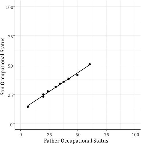
Figure 2. The distribution of occupational status, CCC and CCC2 scores. Note: Each occupation is weighted equally, not by number of observations.

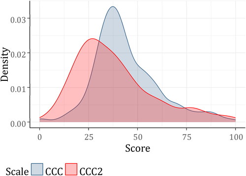
Figure 3. Comparison of CCC and CCC2 scores. Note: The 10 occupations with the highest sum of square deviation between the scores are highlighted.

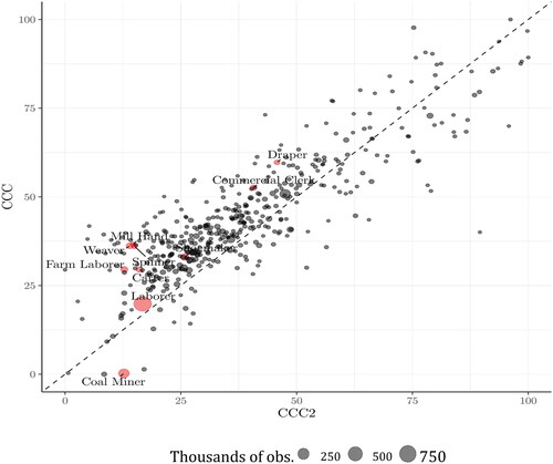
Figure 4. Comparison of HISCAM-GB and CCC-HISCO scores. Note: The ten occupations with the highest sum of square deviation between the scores are highlighted.

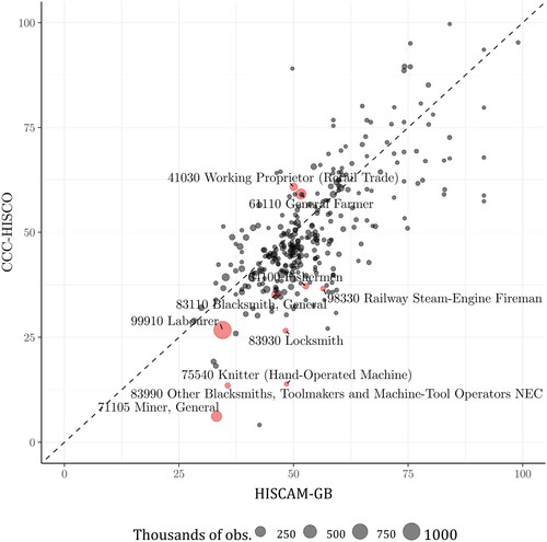
Figure 5. Comparison of HISCAM-U2 and CCC-HISCO scores. Note: The ten occupations with the highest sum of square deviation between the scores are highlighted.

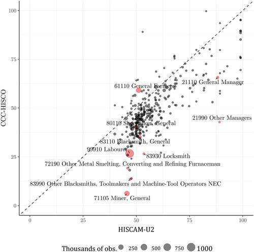
Table A2. The CCC and CCC2 indices and components.

FOE standard occupation	Higher Educ.	Probated	ln Wealth	Literacy 1837–1879	In school 12–18	At work 12–18	CCC	CCC2
Accountant	0.05	0.71	−0.60	0.94	0.55	0.41	61.9	54.2
Actor	0.13	0.41	−1.82	0.88	0.47	0.46	58.6	44.0
Admiral RN	0.20	1.00	2.85	0.85	0.65	0.16	89.2	75.7
Agent	0.04	0.58	−1.30	0.91	0.46	0.43	53.8	47.4
Architect	0.91	0.82	1.00	0.94	0.85	0.15	68.4	86.6
Army	0.22	0.67	−0.51	0.72	0.33	0.39	40.8	48.8
Art Dealer	0.00	0.67	−0.96	0.92	0.23	0.66	59.4	41.0
Artist	0.12	0.71	−0.50	0.93	0.53	0.36	61.1	56.0
Assistant Draper	0.00	0.46	−2.23	0.87	0.38	0.56	50.8	37.6
Assistant Manager	0.03	0.60	−0.70	0.88	0.45	0.55	45.7	46.3
Assistant Teacher	0.55	0.89	0.63	0.87	0.82	0.14	53.3	78.3
Athlete	0.08	0.29	−1.98	0.83	0.90	0.18	30.0	52.2
Attendant	0.02	0.33	−2.13	0.86	0.43	0.59	39.0	36.3
Auctioneer	0.00	0.43	−1.24	0.93	0.59	0.24	63.4	50.4
Author	0.58	0.94	1.49	0.95	0.62	0.19	51.7	79.0
Bailiff	0.00	0.62	−1.39	0.78	0.58	0.54	36.6	45.0
Baker	0.00	0.35	−2.54	0.85	0.30	0.71	41.3	30.5
Bank Accountant	0.00	1.00	−0.01		0.13	0.91	73.1	43.2
Bank Cashier	0.00	0.78	0.07	0.89	0.58	0.38	70.7	56.4
Bank Clerk	0.01	0.84	0.22	0.94	0.55	0.38	67.8	58.5
Bank Manager	0.08	0.88	1.15	0.93	0.70	0.36	73.5	65.8
Bank Messenger	0.00	0.50	−1.63	0.89	0.00	0.35	47.9	36.9
Bank Officer	0.10	0.46	−1.23	0.85	1.00	0.03	73.4	62.3
Banker	0.37	0.91	3.65	0.92	0.60	0.16	80.8	80.2
Barman	0.00	0.23	−2.83	0.77	0.25	0.71	38.9	25.1
Barrister	1.00	0.93	3.02	0.97	0.91	0.09	87.5	98.4
Basket Maker	0.00	0.17	−3.46	0.65	0.36	0.75	33.3	21.2
Bell Hanger	0.00			0.85			39.4
Bellows Maker	0.00			0.61			22.7
Bicycle Maker	0.00	0.40	−0.99	0.85	0.25	0.72	37.2	34.5
Bill Poster	0.00	0.20	−2.59	0.79	0.17	0.88	33.4	21.1
Bishop-Church of England	1.00	0.83	2.04	0.92	1.00	0.14	93.8	93.7
Blade Forger	0.00	0.32	−2.80	0.48	0.10	0.94	25.1	14.1
Bleacher	0.00	0.11	−3.30	0.46	0.37	0.69	39.6	18.0
Boarding House Keeper	0.00	0.67	−0.27	1.00	0.10	0.95	55.9	37.3
Boilermaker	0.00	0.27	−2.79	0.54	0.37	0.60	29.6	25.2
Bookbinder	0.00	0.27	−2.79	0.89	0.40	0.65	44.2	32.0
Bookkeeper	0.01	0.50	−2.21	0.88	0.40	0.56	47.8	39.0
Bookmaker	0.00	0.33	−3.49	0.79	0.61	0.46	40.4	36.3
Bookseller	0.00	0.41	−2.18	0.94	0.43	0.43	61.3	41.5
Bottler	0.00	0.00	−3.52	0.65	0.20	0.96	34.6	11.7
Box Maker	0.00	0.42	−2.38	0.51	0.18	0.77	30.1	21.7
Brass Finisher	0.00	0.25	−2.82	0.73	0.29	0.60	35.1	27.1
Brass Founder	0.00	0.23	−2.84	0.59	0.22	0.82	35.8	19.0
Brass Molder	0.00	0.17	−2.71	0.60	0.72	0.30	34.7	36.8
Brewer	0.13	0.81	1.93	0.73	0.57	0.27	44.7	62.7
Bricklayer	0.00	0.30	−2.62	0.64	0.33	0.64	29.3	26.8
Brickmaker	0.00	0.25	−3.03	0.47	0.11	0.92	22.9	12.8
Brigadier Army	0.75	1.00	1.97		1.00	0.00	70.0	95.8
Broker	0.00	0.74	0.64	0.83	0.64	0.27	56.6	59.1
Brushmaker	0.00	0.23	−3.18	0.73	0.14	0.60	38.9	23.1
Builder	0.00	0.67	−0.74	0.92	0.46	0.39	53.4	50.5
Bus Conductor	0.00	0.27	−2.42	0.86	0.33	0.66	36.5	30.9
Bus Driver	0.00	0.40	−1.84	0.78	0.27	0.65	34.9	32.2
Butcher	0.00	0.44	−1.94	0.85	0.40	0.56	44.5	37.9
Butler	0.00	0.53	−1.73	0.90	0.37	0.67	42.8	38.7
Buyer	0.00	0.63	−1.03	0.85	0.46	0.61	55.6	43.9
Cab Proprietor	0.00	0.33	−2.98	0.81	0.11	0.00	46.0	37.0
Cabinet Maker	0.00	0.33	−2.79	0.85	0.50	0.49	44.6	37.1
Cable Hand	0.00	0.62	−1.26		0.62	0.53	39.0	48.0
Candle Maker	0.00	0.00	−4.33	0.80	0.49	0.70	37.7	22.3
Capstan Operator	0.00	0.00	−2.48		0.00	0.66		12.9
Captain Army	0.36	0.90	1.39	0.96	0.83	0.08	84.3	79.9
Captain RN	0.05	0.93	1.77	0.98	0.48	0.43	80.1	63.7
Carder	0.00	0.13	−2.87	0.36	0.19	0.85	37.0	11.4
Caretaker	0.01	0.45	−2.10	0.79	0.37	0.64	40.0	34.8
Carpenter	0.00	0.33	−2.66	0.82	0.46	0.49	38.0	35.8
Carrier	0.00	0.31	−2.67	0.70	0.23	0.84	33.6	22.8
Carter	0.00	0.18	−3.10	0.47	0.22	0.76	29.5	16.1
Carver and Gilder	0.00	0.29	−2.92	0.84	0.52	0.45	46.5	36.8
Cashier	0.00	0.79	−0.22	0.89	0.41	0.58	58.9	49.2
Castrator	0.00	0.33	−3.14	0.88	0.21	0.79	44.2	26.2
Caulker	0.00	0.25	−2.23	0.75	0.51	0.34	40.8	38.0
Cellarman	0.00	0.21	−3.51	0.76	0.14	0.79	37.5	19.1
Chainmaker	0.00	0.29	−2.69	0.28	0.27	0.70	1.4	17.1
Chair Maker	0.00	0.03	−3.80	0.56	0.20	0.63	36.4	15.3
Chartered Accountant	0.95	0.85	1.01	0.93	0.62	0.37	70.2	79.8
Chauffeur	0.00	0.48	−1.90		0.33	0.58	38.6	35.3
Cheesemonger	0.00	0.40	−2.10	0.95	0.67	0.46	49.9	45.6
Chef	0.00	0.44	−1.40		0.40	0.68	46.5	35.3
Chemist	0.08	0.67	−0.49	0.94	0.74	0.23	61.9	61.0
Chimney Sweep	0.00	0.25	−2.78	0.29	0.29	0.60	23.6	18.4
Cigar Maker	0.00	0.10	−3.94	0.79	0.26	0.68	45.8	21.1
Civil Engineer	0.91	0.79	0.93	0.95	0.83	0.08	71.7	86.9
Civil Servant	0.17	0.81	0.30	0.94	0.64	0.30	56.7	64.3
Civil Servant-Clerk	0.05	0.71	−0.37	0.94	0.43	0.51	56.8	50.9
Civil Servant-High	0.35	0.91	1.18	0.94	0.79	0.25	62.7	75.1
Cleaner	0.00	0.28	−2.36	0.65	0.28	0.67	29.4	26.0
Clergy-Church Of England	0.99	0.89	1.48	0.94	0.86	0.05	85.4	92.4
Clergy-Other	0.52	0.58	−1.12	0.98	0.52	0.45	60.0	59.0
Cloth Finisher	0.00	0.29	−3.08	0.49	0.21	0.81	40.2	17.5
Coach Builder	0.00	0.32	−2.35	0.79	0.52	0.46	42.8	37.8
Coachman	0.01	0.30	−2.92	0.80	0.21	0.77	37.1	25.1
Coal Merchant	0.00	0.62	−1.12	0.83	0.34	0.48	47.0	43.2
Coal Miner	0.00	0.21	−2.81	0.28	0.21	0.79	0.2	12.7
Coal Porter	0.00	0.11	−3.10	0.49	0.23	0.78	29.8	15.1
Coffee House Keeper	0.00	0.35	−2.53	0.92	0.12	0.60	48.6	30.5
Collector	0.02	0.56	−1.77	0.87	0.30	0.58	47.3	38.9
Colliery Owner	0.00	0.88	2.38	0.92	0.26	0.71	59.1	53.5
Colonel Army	0.49	0.93	1.83	0.89	0.66	0.09	90.3	79.3
Color Maker	0.00	0.67	−3.73	0.71	0.49	0.70	39.6	33.4
Commander RN	0.09	0.92	1.27	0.95	0.72	0.24	84.0	70.1
Commercial Artist	0.00	0.42	−1.88	0.92	0.48	0.54	52.7	41.0
Commercial Clerk	0.00	0.57	−1.40	0.89	0.34	0.60	52.6	40.7
Commercial Painter	0.00	0.34	−2.32	0.83	0.31	0.56	40.6	33.2
Commercial Traveler	0.00	0.59	−1.41	0.84	0.44	0.51	54.4	43.4
Commission Agent	0.00	0.33	−2.57	0.90	0.21	0.60	55.3	31.5
Company Director	0.23	0.84	1.36	0.92	0.55	0.34	69.5	65.8
Company Secretary	0.26	0.85	0.88	0.96	0.54	0.40	63.2	64.9
Compositor	0.00	0.42	−2.12	0.86	0.44	0.56	44.7	38.3
Confectioner	0.00	0.56	−1.53	0.83	0.55	0.44	47.4	45.6
Contractor	0.00	0.58	−0.62	0.49	0.37	0.57	44.2	36.0
Convict	0.04	0.00	−4.43		0.09	0.72	29.3	9.6
Cook	0.00	0.22	−3.14	0.84	0.47	0.59	41.4	31.6
Cooper	0.00	0.42	−2.78	0.77	0.61	0.35	37.2	41.2
Coppersmith	0.00	0.46	−1.93	0.77	0.49	0.43	41.5	40.6
Cork Cutter	0.00	0.00	−3.73	0.85	0.07	0.95	39.8	13.0
Cornet Army	0.33	1.00	2.58	1.00	1.00	0.00	40.0	89.6
Corporal Army	0.01	0.26	−2.85	0.84	0.46	0.51	39.4	34.5
Crane Driver	0.00	0.39	−2.10	0.54	0.35	0.69	32.7	27.4
Currier	0.00	0.00	−4.13	0.83	0.45	0.61	43.1	24.1
Customs Officer	0.10	0.71	−0.69	0.96	0.49	0.60	56.2	51.1
Cutler	0.00	0.17	−3.81	0.63	0.17	0.88	37.8	14.2
Dairyman	0.00	0.46	−1.91	0.82	0.21	0.76	42.2	30.9
Deacon-Church of England	1.00	1.00	2.50	0.91	1.00	0.00	89.3	100.0
Dealer	0.00	0.45	−1.99	0.75	0.29	0.62	41.7	32.9
Dentist	0.64	0.63	−0.39	0.92	0.88	0.19	67.1	74.0
Designer	0.03	0.77	−0.32	0.91	0.58	0.43	53.3	55.3
Diplomat	0.60	0.88	1.42	0.85	0.43	0.07	82.4	74.8
Dock Laborer	0.00	0.11	−2.97	0.36	0.37	0.62	28.6	18.1
Domestic Gardener	0.00	0.33	−2.66	0.81	0.25	0.74	32.0	27.7
Doubler	0.00	0.25	−3.78	0.35	0.15	0.85	37.8	9.9
Draper	0.02	0.57	−1.15	0.67	0.59	0.38	59.7	45.8
Draughtsman	0.05	0.63	−0.85	0.88	0.53	0.45	52.4	49.9
Drawer In	0.00	0.25	−3.15	0.55	0.01	1.00	36.6	10.7
Dressmaker	0.00	0.00	−3.69	0.81	0.20	0.78	42.5	17.6
Driller	0.00	0.35	−2.20	0.52	0.18	0.83	32.1	20.2
Drover	0.00	0.00	−4.09	0.61	1.00	0.00	28.2	40.6
Dyer	0.02	0.27	−2.63	0.45	0.23	0.60	40.1	21.7
Electrical Engineer	0.41	0.77	−0.08		0.45	0.38	54.5	60.8
Electrician	0.01	0.54	−1.32	0.87	0.39	0.43	41.4	43.9
Enameller	0.00	0.00	−3.18	0.65	0.18	0.77	30.9	15.6
Engineer	0.13	0.59	−1.01	0.64	0.61	0.35	40.8	48.6
Engraver	0.00	0.46	−1.81	0.81	0.53	0.36	47.4	43.6
Erector	0.00	0.26	−2.20	0.66	0.27	0.65	35.8	26.4
Esquire	0.40	0.96	1.81	0.98	0.73	0.44	97.7	75.3
Estate Agent	0.12	0.81	1.10	0.97	0.60	0.25	66.4	66.4
Factory Hand	0.00	0.32	−2.26	0.42	0.20	0.79	32.5	18.5
Farm Bailiff	0.00	0.45	−2.06	0.75	0.34	0.66	36.0	33.1
Farm Carter	0.00	0.17	−2.78	0.67	0.19	0.84	28.2	18.7
Farm Laborer	0.00	0.15	−3.43	0.47	0.17	0.82	29.6	12.8
Farm-Cowman	0.00	0.29	−2.20	0.60	0.27	0.71	29.7	24.7
Farm-Horseman	0.00	0.33	−2.27	0.57	0.22	0.81	26.4	22.0
Farm-Shepherd	0.00	0.29	−2.75	0.53	0.16	0.75	24.5	18.9
Farm-Stockman	0.00			0.74			30.3	23.4
Farmer	0.02	0.70	−0.58	0.85	0.39	0.50	50.8	47.5
Farmer-Large	0.04	0.74	0.46	0.95	0.49	0.34	76.9	57.9
Farmer-Small	0.00	0.68	−1.96	0.76	0.39	0.56	49.7	40.1
Farmers Son	0.00	0.35	−2.49	0.86	0.36	0.63	55.5	33.3
Farrier	0.00	0.17	−3.18	0.82	0.41	0.45	39.6	31.6
Feltmaker	0.00	0.00	−1.97	0.59	0.35	0.65	30.4	22.7
Fettler	0.00	0.14	−2.76	0.15	0.57	0.47	27.6	21.3
File Cutter	0.00	0.20	−3.33	0.56	0.26	0.79	28.1	17.8
File Forger	0.00	0.57	−2.40	0.92	0.11	0.96	23.4	28.1
File Smith	0.00	0.25	−4.17	0.60	0.00	1.00	34.0	8.7
Filer	0.00	0.10	−2.87	0.47	0.20	0.87	20.0	12.8
Fireman	0.00	0.36	−2.31	0.70	0.33	0.69	30.6	28.9
Fish Curer	0.00	0.14	−3.48	0.51	0.05	0.71	34.0	12.7
Fisherman	0.00	0.20	−3.33	0.55	0.47	0.60	30.7	24.8
Fishmonger	0.00	0.21	−2.92	0.67	0.26	0.80	37.2	21.1
Fitter	0.00	0.44	−1.93	0.70	0.41	0.52	34.9	35.7
Florist	0.00	0.44	−2.80	0.92	0.35	0.68	51.7	34.1
Flying Officer RAF	0.27	0.72	−0.70		0.67	0.30	51.3	61.7
Footman	0.00	0.40	−2.45	0.89	0.09	0.53	34.4	31.8
Foreman	0.00	0.52	−1.55	0.78	0.27	0.70	38.5	34.0
Forester/Woodman	0.00	0.27	−2.95	0.66	0.63	0.30	29.9	37.2
Forgeman	0.00	0.21	−3.06	0.40	0.17	0.89	16.5	12.1
Framework Knitter	0.00	0.19	−3.10	0.52	0.00	1.00	9.2	9.0
French Polisher	0.02	0.28	−2.65	0.69	0.22	0.62	39.8	26.1
Fruiterer	0.04	0.44	−2.19	0.68	0.06	0.84	38.9	23.7
Furnaceman	0.00	0.19	−3.08	0.35	0.15	0.78	15.8	12.1
Furrier	0.00	0.00	−4.45	0.81	0.53	0.43	54.2	27.6
Gamekeeper	0.00	0.35	−2.60	0.77	0.22	0.65	32.4	28.2
Garage Proprietor	0.00	0.75	1.42		0.53	0.12	52.9	63.0
Gardener	0.00	0.34	−2.64	0.79	0.22	0.68	34.4	27.7
Gas Fitter	0.00	0.35	−2.59	0.71	0.37	0.59	36.8	30.9
Gas Worker	0.00	0.00	−3.12	0.45	0.69	0.26	31.6	29.6
Gatekeeper	0.00	0.22	−3.30	0.74	0.20	0.56	33.3	24.8
General Army	0.51	1.00	2.31	0.89	0.58	0.26	90.7	77.8
Gentleman	0.24	0.91	1.80	0.95	0.76	0.00	72.9	78.8
Glass Cutter	0.00	0.00	−3.80	0.68	0.00	0.75	30.6	11.3
Glassblower	0.00	0.10	−3.19	0.53	0.36	0.70	26.4	19.2
Glassmaker	0.00	0.33	−2.56	0.56	0.30	0.70	26.7	24.5
Glazier	0.00	0.11	−2.70	0.79	0.35	0.70	37.5	25.7
Glover	0.00	0.00		0.81	0.00	1.00	39.4	8.3
Goldsmith	0.00	0.15	−3.52	0.79	0.33	0.68	48.8	24.1
Grazier	0.00	1.00	0.73	0.96	0.79	0.36	61.7	67.4
Greengrocer	0.00	0.23	−2.87	0.56	0.33	0.65	33.8	23.0
Grinder	0.00	0.14	−3.15	0.38	0.23	0.79	28.7	12.8
Grocer	0.00	0.58	−1.32	0.92	0.41	0.50	51.0	44.8
Groom	0.00	0.23	−3.11	0.73	0.24	0.79	30.3	21.9
Groundsman	0.00	0.38	−2.34	0.84	0.39	0.20	30.6	41.6
Gunmaker	0.00	0.17	−3.54	0.65	0.35	0.43	35.9	26.4
Hairdresser	0.00	0.33	−2.34	0.85	0.28	0.71	42.0	30.4
Hammerman	0.00	0.14	−3.50	0.59	0.58	0.59	32.8	26.2
Handloom Weaver	0.00	0.00	−4.35	0.35	0.23	0.77	34.5	7.3
Harness Maker	0.00	0.31	−3.18	0.71	0.18	0.38	34.4	28.7
Hatter	0.00	0.39	−2.13	0.62	0.47	0.57	39.6	32.8
Hawker	0.01	0.15	−3.21	0.41	0.33	0.61	26.1	18.8
Head Teacher	0.68	0.90	0.93	0.88	0.82	0.17	70.9	81.4
Horse Keeper	0.00	0.03	−3.71	0.59	0.27	0.61	31.4	17.7
Horse Trainer	0.00	0.50	−0.90	0.61	0.41	0.04	39.7	46.1
Horticulturalist	0.00	0.60	0.07	1.00	0.60	0.40	59.1	55.6
Hosiery Hand	0.00	0.25	−2.68		0.05	0.98	18.1	14.4
Hotel Manager	0.00	0.46	−1.07	0.86	0.55	0.47	56.9	45.1
Hotel Porter	0.00	0.10	−3.00	0.80	0.63	0.50	38.0	33.5
House Decorator	0.00	0.38	−2.06	0.86	0.31	0.59	46.8	34.7
House Furnisher	0.00	0.62	−0.90	0.64	0.16	0.98	54.8	27.9
House Painter	0.00	0.22	−2.87	0.78	0.30	0.64	37.9	27.2
Housekeeper	0.00	0.00	−4.17	0.53	0.61	0.50	37.2	23.1
Hurdle Maker	0.00			0.55			24.7
Innkeeper	0.00	0.62	−1.41	0.89	0.41	0.59	49.4	43.1
Inspector	0.00	0.43	−2.00	0.60	0.30	0.65	41.6	29.1
Instrument Maker	0.00	0.38	−1.74	0.75	0.36	0.49	39.4	36.0
Insurance Agent	0.01	0.55	−1.37	0.84	0.42	0.55	43.1	42.1
Insurance Broker	0.00	0.70	−0.27		0.58	0.49	70.0	52.1
Insurance Inspector	0.00	0.75	−0.91		1.00	0.00	61.6	69.6
Iron Dresser	0.00	0.40	−2.20	0.39	0.11	0.85	29.4	16.7
Iron Molder	0.00	0.26	−2.73	0.52	0.37	0.64	25.4	24.2
Iron Turner	0.00	0.29	−3.03	0.69	0.30	0.73	35.7	24.4
Ironfounder	0.04	0.67	−0.35	0.68	0.39	0.44	40.2	45.3
Ironmaster	0.11	0.89	3.41	0.94	0.79	0.38	67.0	74.2
Ironmonger	0.00	0.67	−0.98	0.94	0.54	0.48	58.2	50.2
Jeweler	0.01	0.49	−1.54	0.83	0.61	0.26	53.4	48.9
Journalist	0.08	0.62	−1.09	0.91	0.53	0.23	60.5	54.1
Judge	0.92	0.88	2.60	1.00	1.00	0.00	88.2	98.6
Justice of the Peace	0.57	0.91	2.61	0.92	0.85	0.03	85.3	87.8
Laborer	0.00	0.18	−3.00	0.43	0.26	0.71	19.9	16.8
Lace Hand	0.00	0.50	−0.86	0.83	0.02	0.98	36.9	27.3
Lace Maker	0.00	0.17	−3.67	0.75	0.42	0.58	32.7	26.6
Lamplighter	0.00	0.22	−3.09	0.69	0.20	0.85	29.6	19.3
Landed Proprietor	0.43	0.86	2.64	0.91	0.88	0.07	68.3	83.9
Laundry Worker	0.00	0.00	−3.53	0.65	0.24	0.39	37.1	22.2
Leather Worker	0.00	0.41	−2.39	0.77	0.30	0.65	39.8	31.1
Legal Clerk	0.01	0.52	−1.79	0.94	0.33	0.67	54.6	38.6
Librarian	0.00	0.71	−0.43	0.82	0.30	0.38	59.5	47.2
Licensed Victualer	0.00	0.61	−1.15	0.84	0.44	0.54	43.8	44.0
Lieutenant Army	0.39	0.77	0.24	0.96	0.70	0.20	79.7	70.7
Lieutenant Commander RN	0.31	0.88	1.23		0.96	0.31	75.1	77.6
Lieutenant RN	0.06	0.85	0.49	0.97	0.38	0.40	77.1	57.6
Lieutenant-Colonel Army	0.43	0.91	1.39	0.97	0.78	0.06	87.6	81.2
Lineman	0.00	0.36	−2.44	0.70	0.37	0.74	35.0	28.6
Locksmith	0.00	0.25	−3.15	0.41	0.07	0.00	18.6	26.0
Loco Driver	0.00	0.46	−2.01	0.75	0.27	0.69	30.4	31.4
Lorry Driver	0.00	0.32	−1.90		0.38	0.60	31.9	32.1
Machine Ruler	0.00	0.20	−2.77	1.00	0.44	0.70	46.2	33.1
Machinist	0.00	0.32	−2.22	0.68	0.28	0.65	36.9	28.0
Magistrate	0.59	0.94	3.44	0.89	1.00	0.00	86.2	93.5
Major Army	0.46	0.90	1.42	0.94	0.81	0.12	87.3	80.3
Malster	0.00	0.50	−1.68	0.71	0.46	0.56	36.4	37.9
Manager	0.05	0.67	−0.59	0.83	0.51	0.45	50.8	50.0
Manufacturer	0.03	0.70	0.36	0.89	0.58	0.47	60.4	54.7
Mariner	0.00	0.21	−3.27	0.71	0.43	0.55	39.0	28.3
Mariner Mate	0.00	0.55	−1.74	0.88	0.52	0.36	52.4	46.7
Market Gardener	0.00	0.60	−1.17	0.80	0.29	0.68	40.0	37.7
Mason	0.00	0.28	−3.17	0.66	0.39	0.62	32.1	26.9
Master Baker	0.00	0.59	−1.30	0.97	0.07	0.71	53.2	36.0
Master Mariner	0.01	0.59	−1.27	0.92	0.63	0.28	53.6	53.0
Mattress Maker	0.00	0.43	−1.86	0.76	0.05	0.97	33.2	22.6
Mechanic	0.00	0.43	−1.90	0.65	0.41	0.56	40.4	34.0
Mechanical Engineer	0.19	0.70	−0.45	0.89	0.62	0.30	51.4	59.3
Medical Attendant	0.00	0.17	−3.17	0.81	0.32	0.48	37.8	29.3
Medical Doctor	0.97	0.86	1.02	0.97	0.77	0.11	78.7	88.4
Member of Parliament	0.75	0.95	4.52	0.99	0.91	0.02	96.7	99.8
Merchant	0.06	0.78	1.00	0.92	0.57	0.37	66.0	60.7
Merchant Seaman	0.00	0.24	−2.78	0.67	0.38	0.54	33.6	28.6
Messenger	0.00	0.31	−2.35	0.88	0.17	0.84	41.5	26.3
Midshipman RN	0.00	0.80	−0.03		0.33	0.67	64.6	46.6
Milkman	0.00	0.23	−2.49	0.75	0.13	0.73	34.0	23.1
Mill Hand	0.00	0.24	−2.93	0.50	0.15	0.88	36.6	14.6
Miller	0.00	0.34	−2.67	0.83	0.34	0.70	41.9	30.5
Milliner	0.00	1.00	0.42	0.55	0.53	0.43	40.2	52.4
Millwright	0.00	0.46	−2.13	0.78	0.73	0.33	40.2	46.3
Mine Agent	0.00	0.67	−1.76	0.90	0.84	0.27	35.8	56.4
Mine Laborer	0.00	0.26	−2.81		0.29	0.74	14.6	23.6
Miner	0.00	0.21	−3.19	0.40	0.16	0.84	17.1	12.4
Mining Engineer	0.31	0.67	−0.15	0.81	0.44	0.37	59.3	55.7
Model Maker	0.00	0.67	−0.90	0.95	0.47	0.58	43.8	47.8
Motor Driver	0.00	0.25	−2.29		0.24	0.59	34.5	26.4
Musical Instrument Maker	0.00	0.67	−2.09	0.78	0.00	1.00	22.3	25.0
Musician	0.03	0.50	−2.07	0.79	0.39	0.58	47.2	37.5
Nail Forger	0.00	0.00	−4.37	0.29	0.14	0.80	15.6	3.7
Nailer	0.00	0.07	−3.76	0.28	0.24	0.78	0.0	8.4
Newsagent	0.00	0.71	−0.83	0.70	0.39	0.59	41.7	41.8
None	0.22	0.43	−1.00	0.96	0.49	0.07	43.2	56.8
Nurse	0.00	0.33	−2.56	0.67	0.41	0.66	41.4	29.2
Nurseryman	0.00	0.56	−0.88	0.93	0.29	0.58	50.8	42.0
Officer Army	0.42	0.85	0.46	0.98	0.61	0.16	69.4	72.7
Officer RN	0.08	0.65	−0.40	0.85	0.79	0.24	59.3	59.8
Oiler	0.10	0.57	−1.76	0.65	0.12	0.69	32.3	31.1
Optician	0.67	0.67	−0.34	0.79	0.26	0.66	54.4	53.2
Ore Dresser	0.00	0.00	−4.32	0.43	0.00	1.00	0.3	0.7
Outfitter	0.00	0.83	0.26	0.91	0.55	0.33	60.6	58.5
Own Means	0.27	0.84	1.43	0.94	0.77	0.06	60.0	76.1
Packer	0.00	0.28	−2.56	0.66	0.15	0.72	36.0	22.4
Packing Case Maker	0.00	0.43	−1.96	0.62	0.27	0.52	38.2	31.5
Paper Hanger	0.00	0.29	−2.97	0.81	0.21	0.62	39.2	27.3
Paper Maker	0.00	0.38	−2.12	0.66	0.34	0.76	35.0	28.1
Paper Stainer	0.00	0.50	−2.31	0.62	0.16	0.77	46.4	25.1
Parish Clerk	0.00	0.50	−2.74	0.86	0.48	0.60	33.7	37.9
Pattern Maker	0.00	0.45	−1.82	0.84	0.46	0.58	41.6	38.8
Pauper	0.00	0.04	−8.34	0.49	0.21	0.58	20.5	2.7
Paver	0.00	0.17	−2.97	0.41	0.00	0.68	34.4	12.1
Pawnbroker	0.00	0.67	1.10	0.90	0.68	0.38	57.7	59.4
Petty Officer Army	0.00	0.63	−1.75	0.89	0.26	0.55	49.6	40.1
Petty Officer RN	0.02	0.44	−2.41	0.92	0.48	0.60	45.6	39.1
Photographer	0.02	0.46	−2.02	0.86	0.58	0.35	51.8	45.6
Piano Maker	0.00	0.58	−1.82	0.89	0.29	0.71	44.0	36.9
Piano Tuner	0.00	0.50	−1.33	0.85	0.54	0.17	48.4	50.0
Picture Framer	0.00	0.40	−2.47	0.84	0.56	0.55	42.6	38.6
Pipe Fitter	0.00	0.33	−2.05	0.61	0.00	1.00	30.8	16.0
Pipe Maker	0.00	0.14	−3.24	0.58	0.30	0.58	24.0	22.0
Plasterer	0.00	0.27	−2.62	0.69	0.29	0.61	34.1	27.4
Platelayer	0.00	0.28	−2.97	0.61	0.17	0.74	27.1	20.3
Plater	0.00	0.21	−3.08	0.68	0.80	0.33	33.1	38.9
Plumber	0.00	0.45	−2.06	0.86	0.40	0.55	43.1	38.1
Police Constable	0.00	0.44	−2.25	0.87	0.34	0.65	35.4	35.0
Police Officer	0.00	0.52	−1.74	0.89	0.58	0.41	43.7	46.6
Police Sergeant	0.00	0.77	−1.09	0.87	0.29	0.64	44.5	42.7
Polisher	0.00	0.28	−2.65	0.52	0.26	0.83	29.2	19.4
Porter	0.00	0.23	−2.82	0.75	0.26	0.67	33.0	25.5
Postman	0.00	0.49	−1.79	0.77	0.28	0.68	35.9	33.3
Postmaster	0.05	0.83	−0.15	0.90	0.23	0.56	54.9	48.4
Potter	0.00	0.28	−2.88	0.48	0.27	0.76	12.8	19.1
Pottery Decorator	0.00	0.67	−0.47	0.80	0.42	0.69	39.0	42.8
Poulterer	0.00	0.50	−2.16	0.83	0.33	0.78	44.3	32.9
Presser	0.00	0.22	−2.79	0.52	0.03	0.57	28.0	18.3
Printer	0.00	0.43	−2.13	0.72	0.54	0.42	44.0	39.6
Printer Compositor	0.00	0.41	−2.08		0.38	0.60	52.6	33.8
Printers Assistant	0.03	0.45	−1.87	1.00	0.24	0.67	38.5	37.3
Printers Cutter	0.00	0.00	−3.06	1.00	0.12	0.84	45.6	20.5
Printers Reader	0.00	0.33	−1.84	0.74	0.45	0.60	54.9	34.5
Professor	0.92	0.92	1.15	0.93	0.70	0.25	67.1	84.2
Publisher	0.33	0.83	2.56	0.93	0.47	0.53	66.4	66.2
Puddler	0.00	0.07	−3.81	0.28	0.27	0.69	10.7	10.3
Quarryman	0.00	0.27	−2.76	0.46	0.24	0.69	27.6	19.7
RAF		0.60					43.1
Rag Sorter	0.00	0.00	−4.03	0.31	0.19	0.85	41.8	5.2
Railway Guard	0.00	0.44	−2.18	0.83	0.20	0.67	37.1	31.4
Railway Signalman	0.00	0.37	−2.34	0.82	0.26	0.66	34.1	30.9
Railway Stoker	0.00	0.46	−1.80	0.90	0.34	0.36	31.9	42.0
Railway Worker	0.00	0.33	−2.19	0.80	0.19	0.55	34.5	30.8
Refuse Collector	0.00	0.27	−2.69	0.39	0.18	0.69	30.6	17.3
Restaurant Keeper	0.00	0.73	−1.17	0.90	0.42	0.46	49.4	48.1
Riveter	0.00	0.18	−2.74	0.58	0.51	0.60	24.1	27.3
Ropemaker	0.00	0.25	−2.99	0.61	0.34	0.69	36.1	23.8
Royal Navy	0.00			0.76			43.9
Saddler	0.00	0.40	−2.42	0.87	0.60	0.48	45.6	41.3
Sailmaker	0.00	0.29	−3.14	0.84	0.61	0.40	42.7	38.6
Salesman	0.01	0.54	−1.20	0.87	0.37	0.57	51.0	41.7
Sawyer	0.00	0.19	−3.19	0.60	0.35	0.60	29.0	23.9
Scaffolder	0.00	0.33	−2.67		0.10	0.87	33.3	19.4
Scientist	0.64	0.80	0.39	0.87	0.60	0.40	60.0	69.3
Seaman RN	0.00	0.25	−2.71	0.79	0.38	0.57	35.7	30.9
Secretary	0.11	0.57	−1.37	0.89	0.47	0.45	61.1	47.8
Sergeant Army	0.00	0.28	−2.73	0.89	0.32	0.64	43.9	31.0
Servant	0.01	0.31	−3.04	0.72	0.21	0.79	30.2	23.0
Sheet Metal Worker	0.00	0.54	−1.59	0.60	0.49	0.45	32.2	39.2
Shingler	0.00	0.40	−2.46	0.46	0.43	0.61	17.1	27.7
Ships Steward	0.00	0.15	−2.99	0.86	0.62	0.47	43.7	36.2
Shipwright	0.00	0.33	−2.80	0.83	0.61	0.39	41.3	40.1
Shoemaker	0.00	0.27	−3.05	0.70	0.33	0.68	33.1	25.8
Shop Assistant	0.00	0.36	−2.17	0.83	0.26	0.66	40.4	31.3
Shop Manager	0.01	0.63	−1.22	0.85	0.27	0.66	47.5	39.2
Shopkeeper	0.00	0.65	−1.29	0.88	0.31	0.66	43.1	40.3
Sign Writer	0.00	0.61	−0.97	0.92	0.22	0.43	47.1	44.0
Skinner	0.00	0.33	−1.57	0.67	0.00	1.00	34.3	18.5
Slater	0.00	0.13	−3.46	0.55	0.23	0.53	33.3	20.1
Slaughterman	0.00	0.33	−1.57	0.71	0.26	0.71	33.6	29.3
Smith	0.00	0.27	−2.85	0.67	0.32	0.67	30.0	25.6
Soap Maker	0.00	0.50	−2.36	0.76	0.49	0.70	38.6	35.2
Soldier Army	0.01	0.25	−2.81	0.70	0.35	0.61	34.4	27.7
Solicitor	0.98	0.86	1.53	0.96	0.79	0.14	79.6	89.5
Sorter Post Office	0.00	0.82	−0.88	0.85	0.17	0.87	45.9	37.7
Spade Maker	0.00	0.60	−0.78	0.47	0.21	0.88	14.2	27.0
Spinner	0.00	0.24	−2.92	0.41	0.21	0.82	36.1	15.0
Spring Maker	0.00	0.38	−3.11	0.59	0.27	0.77	29.4	22.4
Stamper	0.00	0.22	−2.87	0.52	0.25	0.63	23.4	21.2
Station Master	0.00	0.54	−1.84	0.90	0.41	0.60	52.2	40.3
Stationary Engineman	0.00	0.27	−2.77	0.61	0.22	0.78	28.8	21.1
Stationer	0.03	0.75	−0.28	0.94	0.47	0.29	60.1	56.0
Stay Maker	0.00	0.00	−4.34	0.72	0.53	0.43	44.4	26.0
Steelworker	0.00	0.32	−2.56	0.48	0.18	0.69	18.2	20.5
Stenographer	0.00	1.00	1.00	0.85	0.15	0.82	63.2	46.3
Steward	0.00	0.40	−1.87	0.86	0.36	0.60	43.8	36.1
Stick Maker	0.00	0.00	−3.86	0.40	0.05	0.85	38.1	4.8
Stillman	0.00	0.00	−3.18	0.00			27.4
Stockbroker	0.10	0.87	1.87	0.95	0.73	0.18	75.0	72.1
Stoker	0.00	0.29	−2.54	0.59	0.40	0.66	28.0	26.8
Storekeeper	0.00	0.54	−1.71	0.72	0.24	0.77	37.3	31.0
Striker	0.00	0.20	−2.91	0.41	0.31	0.71	24.0	18.0
Student	0.81	0.82	0.42	0.94	0.84	0.10	73.1	83.9
Supervisor	0.03	0.60	−1.24		0.40	0.33	53.3	46.3
Surveyor	0.13	0.66	−0.75	0.95	0.55	0.44	58.4	54.1
Tailor	0.00	0.28	−2.84	0.81	0.53	0.43	39.2	36.8
Tailors Cutter	0.00	0.38	−2.07	0.78	0.35	0.65	46.1	32.8
Tallow Chandler	0.00	0.56	−1.68	0.85	0.39	0.21	43.5	46.6
Tanner	0.03	0.14	−3.22	0.66	0.30	0.77	37.5	20.8
Tax Assessor	0.33	0.33	−2.00	0.98	0.92	0.11	68.1	62.2
Tax Collector	0.00	0.91	−0.74	0.89	0.43	0.32	57.3	54.6
Taxi Driver	0.00	0.36	−1.67		0.00	0.41	40.8	28.5
Taxidermist	0.00	0.50	−0.88	1.00	1.00	0.00	43.5	65.6
Tea Planter	0.11	0.82	0.45	0.80	0.69	0.01	79.2	66.9
Teacher	0.34	0.72	−0.61	0.93	0.74	0.25	54.3	66.2
Teacher Elementary	0.00	0.86	−0.25	0.98	0.61	0.29	50.9	60.6
Technician	0.03	0.51	−1.28	0.68	0.44	0.51	45.5	39.6
Telegraphist	0.00	0.58	−1.33	0.84	0.33	0.49	49.0	41.7
Telephonist	0.00	0.56	−1.23		0.10	1.00	34.5	26.4
Textile Twister	0.00	0.50	−1.41	0.45	0.13	0.93	36.9	21.0
Thatcher	0.00	0.17	−3.08	0.64	0.14	0.80	25.8	17.1
Theatre And Film	0.24	0.58	−0.58	0.51	0.59	0.36	50.1	48.6
Ticket Collector	0.00	0.25	−2.74	0.82	0.00	1.00	41.8	17.0
Tiler	0.00	0.25	−2.65	0.61	0.20	0.90	31.8	18.6
Timber Merchant	0.00	0.70	−0.41	0.90	0.34	0.44	58.8	48.4
Time Keeper	0.00	0.44	−1.28	0.81	0.10	0.81	39.9	29.2
Tin Plate Worker	0.02	0.26	−2.88	0.68	0.18	0.77	31.4	21.8
Tinsmith	0.00	0.23	−2.26	0.61	0.30	0.63	35.5	25.7
Titled	0.48	0.97	4.53	0.95	1.00	0.00	100.0	96.2
Tobacco Worker	0.00	0.00	−3.62	0.93	0.09	0.90	37.6	16.0
Tobacconist	0.00	0.53	−1.37	0.88	0.75	0.10	53.2	55.9
Toolmaker	0.00	0.51	−1.62	0.58	0.33	0.57	31.7	33.0
Tradesman	0.00	0.24	−2.83	0.62	0.45	0.53	34.6	29.0
Trainer	0.00	0.38	−1.30	0.79	0.45	0.28	41.7	43.3
Tram Driver	0.00	0.39	−1.75	0.42	0.02	0.67	39.5	19.8
Trimmer	0.00	0.20	−2.82	0.70	0.37	0.63	31.7	26.8
Tripe Dresser	0.00	0.50	−1.21	0.45	0.63	0.44	37.1	39.0
Turncock	0.00	0.20	−2.79	0.88	0.37	0.71	35.9	29.1
Turner	0.00	0.35	−2.19	0.61	0.34	0.65	33.8	28.5
Typist	0.00	0.33	−2.26		0.07	0.78	50.1	21.4
Umbrella Maker	0.00	0.50	−1.12	0.38	0.39	0.66	38.3	29.6
Undertaker	0.00	0.00	−3.08	0.81	1.00	0.00	50.4	47.4
Unemployed	0.09	0.11	−2.49	0.74	0.52	0.50	43.9	33.8
Upholsterer	0.00	0.33	−2.39	0.88	0.35	0.59	49.9	34.2
Valet	0.00	0.00	−2.88	0.89	0.14	0.83	44.3	19.4
Varnish Maker	0.00	0.00	−2.37	0.73	0.02	1.00	38.7	12.4
Veterinarian	0.88	0.60	−1.24	0.94	0.86	0.16	60.2	76.4
Waiter	0.00	0.16	−2.76	0.83	0.37	0.68	41.3	28.0
Warehouseman	0.00	0.28	−2.49	0.78	0.27	0.72	43.4	27.2
Warper	0.00	0.23	−3.09	0.63	0.27	0.73	40.5	21.4
Watchmaker	0.00	0.42	−2.28	0.75	0.42	0.49	46.2	36.4
Watchman	0.00	0.37	−2.31	0.50	0.23	0.75	32.0	22.2
Waterman	0.00	0.28	−2.88	0.45	0.37	0.69	25.0	21.8
Weaver	0.00	0.23	−3.38	0.43	0.21	0.82	36.2	14.0
Weighman	0.00	0.00	−3.00	0.55	0.30	0.34	20.6	23.4
Welder	0.00	0.33	−1.28	0.40	0.13	0.84	24.7	19.0
Wharfinger	0.14	1.00	1.28	0.90	0.40	0.66	52.7	58.2
Wheelwright	0.00	0.46	−2.21	0.80	0.53	0.38	36.3	41.9
White Smith	0.00	0.35	−3.08	0.68	0.43	0.57	32.6	30.2
Winder	0.00	0.00	−4.45	0.42	0.00	1.00	29.4	0.0
Window Cleaner	0.00	0.16	−2.61		0.31	0.65	35.5	23.7
Wine Merchant	0.01	0.81	1.21	0.96	0.64	0.27	69.2	64.6
Wire Drawer	0.00	0.22	−3.19	0.59	0.23	0.82	34.8	18.0

Table 1. Father-son occupational pairings, 1837–1879.

Father/Son	Farmer	Farm-worker	Non-farm
Farmer	28,843	1,601	42,433
Farm-worker	187	7,239	8,253
Non-farm	8,078	5,277	814,366

Note: The rows show the numbers of fathers in each occupational category, and the columns the sons.

Source: Marriages of England (MOE) database, 1837–1879.

Table 2. Parish register marriage data, 1837–2021.

Marriage period	All	Groom literacy	Groom occupation	Father occupation	Father-in-law occupation
1837–1859	540,650	289,772	450,905	413,638	411,789
1860–1879	365,465	195,597	310,321	294,935	295,259
1880–1899	336,124	–	285,405	253,004	273,058
1900–1939	343,344	–	283,040	242,408	273,831
1940–1979	66,636	–	61,454	52,986	54,405
1980–2021	15,535	–	15,449	13,786	14,010
All	1,667,754	485,369	1,406,574	1,270,757	1,322,352

Table 3. FOE social status data, males.

Birth period	Occupation	Probate	Ln Wealth	Higher education	Schooling 12–18
1780–1839	12,367	7,084	6,807	11,774	1,440
1840–1879	16,045	10,234	10,170	15,507	5,959
1880–1919	14,264	10,574	10,269	13,585	3,390
All	42,676	27,892	28,148	40,866	10,789

Table 4. Correlations between the components of the CCC2 index.

Component	Fraction literate	Fraction higher education	Fraction probated	Log wealth	Fraction in school 12–18
Fraction literate	–
Fraction higher education	0.356	–
Fraction probated	0.590	0.544	–
Log Wealth	0.569	0.627	0.920	–
Fraction in school 12–18	0.513	0.617	0.617	0.628	–
Fraction at work 12–18	−0.458	−0.560	−0.560	−0.600	−0.885

Table 5. Top and bottom 10 occupations by CCC2 score.

Rank occupation	CCC2 probated wealth educated schooled working literate
1 Deacon-Church of England	100.00	1.00	2.50	1.00	1.00	0.00	0.91
2 Member of Parliament	99.82	0.95	4.52	0.75	0.91	0.02	0.99
3 Judge	98.59	0.88	2.60	0.92	1.00	0.00	1.00
4 Barrister	98.36	0.93	3.02	1.00	0.91	0.09	0.97
5 Titled	96.16	0.97	4.53	0.48	1.00	0.00	0.96
6 Brigadier Army	95.82	1.00	1.97	0.75	1.00	0.00
7 Bishop-Church of England	93.70	0.83	2.04	1.00	1.00	0.14	0.92
8 Magistrate	93.47	0.94	3.44	0.59	1.00	0.00	0.88
9 Clergy-Church of England	92.38	0.89	1.48	0.99	0.86	0.05	0.94
10 Cornet Army	89.56	1.00	2.58	0.33	1.00	0.00	1.00
447 File Smith	8.73	0.25	−4.17	0.00	0.00	1.00	0.60
448 Nailer	8.44	0.07	−3.76	0.00	0.24	0.78	0.28
449 Glover	8.34	0.00		0.00	0.00	1.00	0.81
450 Handloom Weaver	7.26	0.00	−4.35	0.00	0.23	0.76	0.35
452 Stick Maker	4.84	0.00	−3.86	0.00	0.05	0.85	0.40
453 Nail Forger	3.70	0.00	−4.37	0.00	0.14	0.80	0.29
454 Pauper	2.74	0.04	−8.34	0.00	0.21	0.58	0.49
455 Ore Dresser	0.66	0.00	−4.32	0.00	0.00	1.00	0.43
456 Winder	0.00	0.00	−4.45	0.00	0.00	1.00	0.42

Table 6. Top and bottom 10 ranked occupations by CCC score.

Rank	Occ standard	CCC	CCC2
1	Titled	100.00	96.16
2	Esquire	97.69	75.28
3	Member of Parliament	96.73	99.82
4	Bishop-Church of England	93.79	93.70
5	General Army	90.71	77.81
6	Colonel Army	90.33	79.31
7	Deacon-Church of England	89.29	100.00
8	Admiral RN	89.23	75.74
9	Judge	88.18	98.59
10	Lieutenant-Colonel Army	87.57	81.19
453	Nail Forger	15.59	3.70
454	Mine Laborer	14.63	23.55
455	Spade Maker	14.24	27.04
456	Potter	12.79	19.07
458	Framework Knitter	9.19	9.05
459	Chainmaker	1.38	17.07
460	Ore Dresser	0.33	0.66
461	Coal Miner	0.23	12.71
462	Nailer	0.00	8.44

Table 7. Estimating potential biases in the CCC index, marriage sample, 1837–1939.

Pair	Data	CCC (full sample)	CCC (50% sample)
Father-Son	Marriages, full	0.6745	0.6746
Father-Son	Marriages, test 50%	0.6746	0.6749
Father-Son	Marriages, training 50%	0.6745	0.6742
FinL-Groom	Marriages, full	0.5582	0.5584
FinL-Groom	Marriages, test 50%	0.5579	0.5584
FinL-Groom	Marriages, training 50%	0.5586	0.5584

Note: The table shows the calculated father-son correlation in social status, in cases where the CCC index used the full sample, or just a 50% sample distinct from the testing 50% sample. FinL indicates father-in-law.

Table 8. Correlation between occupational status indices, 1800–1939.

Measure	HISCAM-U2	HISCAM-GB	CCC	CCC2	CCC-HISCO
HISCAM-U2	1	0.780	0.697	0.759	0.709
HISCAM-GB		1	0.804	0.791	0.824
CCC			1	0.873	0.976
CCC2				1	0.856
CCC-HISCO					1

Source: FOE and MOE databases.

Table 9. Intergenerational correlations in marriage database, 1837–1939, males.

Group	Period	HISCAM-U2	HISCAM-GB	CCC	CCC2	CCC-HISCO
Father-Son	All	0.514	0.540	0.675	0.627	0.641
Father-Son	1837–1859	0.533	0.591	0.708	0.655	0.674
Father-Son	1860–1899	0.528	0.548	0.679	0.635	0.643
Father-Son	1900–1939	0.447	0.441	0.604	0.555	0.580
Father-FinL	All	0.327	0.351	0.505	0.471	0.442
Father-FinL	1837–1859	0.316	0.379	0.533	0.489	0.466
Father-FinL	1860–1899	0.332	0.355	0.510	0.482	0.442
Father-FinL	1900–1939	0.300	0.292	0.444	0.414	0.400

Note: FinL indicates father-in-law.

Table 10. Father-son correlation of occupation rank (CCC), by location, 1837–1939.

Location	Observations	Intergenerational correlation	Standard error
Kent	134,435	0.650	0.002
Lancashire	173,661	0.561	0.002
Lincolnshire	125,385	0.668	0.002
Staffordshire	166,418	0.646	0.002
All other	650,171	0.676	0.001
All	1,250,070	0.675	0.001

Source: MOE database.

References

- Abramitzky, R., L. Platt Boustan, and K. Eriksson. 2012. Europe’s tired, poor, huddled masses: Self-selection and economic outcomes in the age of mass migration. The American Economic Review 102 (5):1832–56. doi: 10.1257/aer.102.5.1832.
- Bailey, R. E., T. J. Hatton, and K. Inwood. 2016. Health, height, and the household at the turn of the twentieth century. The Economic History Review 69 (1):35–53. doi: 10.1111/ehr.12099.
- Brea-Martínez, G., and J.-M. Pujadas-Mora. 2018. Estimating long-term socioeconomic inequality in southern Europe: The Barcelona area, 1481–1880. European Review of Economic History 23 (4):397–420. doi: 10.1093/ereh/hey017.
- Clark, G. 2023. The inheritance of social status: England, 1600 to 2022. Proceedings of the National Academy of Sciences of the United States of America 120 (27):e2300926120. doi: 10.1073/pnas.2300926120.
- Clark, G., and N. Cummins. 2023. Hypergamy revisited: Marriage in England, 1837–2021. Discussion Papers on Economics, University of Southern Denmark, Department of Economics, Odense.
- Clark, G., N. Cummins, and M. Curtis. 2022. The mismeasure of man: Why intergenerational occupational mobility is much lower than conventionally measured, England, 1800–2021. Technical Report DP17346, Centre for Economic Policy Research, London.
- Connor, D. S. 2017. Poverty, religious differences, and child mortality in the early twentieth century: The case of Dublin. Annals of the American Association of Geographers 107 (3):625–46. doi: 10.1080/24694452.2016.1261682.
- Connor, D. S. 2019. The cream of the crop? Geography, networks, and Irish migrant selection in the age of mass migration. The Journal of Economic History 79 (1):139–75. doi: 10.1017/S0022050718000682.
- Cummins, N. 2020. The micro-evidence for the Malthusian system. France, 1670–1840. European Economic Review 129 (C):103544. doi: 10.1016/j.euroecorev.2020.103544.
- Debiasi, E., and M. Dribe. 2020. SES inequalities in cause-specific adult mortality: A study of the long-term trends using longitudinal individual data for Sweden (1813–2014). European Journal of Epidemiology 35 (11):1043–56. doi: 10.1007/s10654-020-00685-6.
- Dribe, M., and J. Helgertz. 2016. The lasting impact of grandfathers: Class, occupational status, and earnings over three generations in Sweden, 1815–2011. The Journal of Economic History 76 (4):969–1000. doi: 10.1017/S0022050716000991.
- Dribe, M., and L. Quaranta. 2020. The Scanian Economic-Demographic Database (SEDD). Historical Life Course Studies 9:158–72. doi: 10.51964/hlcs9302.
- Dribe, M., and O. Karlsson. 2022. Inequality in early life: Social class differences in childhood mortality in southern Sweden, 1815–1967. The Economic History Review 75 (2):475–502. doi: 10.1111/ehr.13089.
- Erikson, R., and J. H. Goldthorpe. 1992. The constant flux: A study of class mobility in industrial societies. Oxford: Clarendon Press.
- Espín-Sánchez, J.-A., S. Gil-Guirado, W. D. Giraldo-Paez, and C. Vickers. 2019. Labor income inequality in pre-industrial Mediterranean Spain: The city of Murcia in the 18th century. Explorations in Economic History 73:101274. doi: 10.1016/j.eeh.2019.05.002.
- Feigenbaum, J. J. 2018. Multiple measures of historical intergenerational mobility: Iowa 1915 to 1940. The Economic Journal 128 (612):F446–81. doi: 10.1111/ecoj.12525.
- Fernihough, A. 2017. Human capital and the quantity-quality trade-off during the demographic transition. Journal of Economic Growth 22 (1):35–65. doi: 10.1007/s10887-016-9138-3.
- Goodman, L. 1979. Simple models for the analysis of association in cross-classifications having ordered categories. Journal of the American Statistical Association 74 (367):537–52. doi: 10.2307/2286971.
- Hällsten, M., and M. Kolk. 2023. The shadow of peasant past: Seven generations of inequality persistence in Northern Sweden. American Journal of Sociology 128 (6):1716–60. doi: 10.1086/724835.
- Haskey, J. 2015. Marriage rites: Trends in marriages by manner of solemnisation and denomination in England and Wales, 1841–2012. In Marriage rites and rights, ed. R. Probert. London: Hart Publishing.
- Hendrickx, J. 2004. RC2: Stata module to estimate Goodman’s row and columns model 2, statistical software components. Boston, USA: Boston College, Department of Economics.
- Hotelling, H. 1933. Analysis of a complex of statistical variables into principal components. Journal of Educational Psychology 24 (6):417–41, 498–520. doi: 10.1037/h0070888.
- Inwood, K., C. Minns, and F. Summer Eld. 2019. Occupational income scores and immigrant assimilation. Evidence from the Canadian census. Explorations in Economic History 72:114–22. doi: 10.1016/j.eeh.2019.02.001.
- Jaadla, H., E. Potter, S. Keibek, and R. Davenport. 2020. Infant and child mortality by socio-economic status in early nineteenth-century England. Economic History Review 73 (4):991–1022.
- Knigge, A. 2016. Beyond the parental generation: The influence of grandfathers and greatgrandfathers on status attainment. Demography 53 (4):1219–44. doi: 10.1007/s13524-016-0486-6.
- Knigge, A., M. H. D. Van Leeuwen, and I. Maas. 2014. Sources of sibling (dis) similarity: Total family impact on status variation in the Netherlands in the nineteenth century. American Journal of Sociology 120 (3):908–48. doi: 10.1086/679104.
- Knigge, A., M. H. D. Van Leeuwen, I. Maas, and K. Mandemakers. 2014. Status attainment of siblings during modernization. American Sociological Review 79 (3):549–74. doi: 10.1177/0003122414529586.
- Lambert, P. S., R. L. Zijdeman, M. H. D. Van Leeuwen, I. Maas, and K. Prandy. 2013. The construction of HISCAM: A stratification scale based on social interactions for historical comparative research. Historical Methods: A Journal of Quantitative and Interdisciplinary History 46 (2):77–89. doi: 10.1080/01615440.2012.715569.
- Lan, T., and P. A. Longley. 2021. Urban morphology and residential differentiation across Great Britain, 1881–1901. Annals of the American Association of Geographers 111 (6):1–20. doi: 10.1080/24694452.2020.1859982.
- Pearson, K. 1901. On lines and planes of closest t to systems of points in space. Philosophical Magazine 2 (11):559–72. doi: 10.1080/14786440109462720.
- Prandy, K., and P. Lambert. 2003. Marriage, social distance and the social space: An alternative derivation and validation of the Cambridge scale. Sociology 37 (3):397–411. doi: 10.1177/00380385030373001.
- Rosenbaum-Feldbrügge, M. 2019. The impact of parental death in childhood on sons’ and daughters’ status attainment in young adulthood in the Netherlands, 1850–1952. Demography 56 (5):1827–54. doi: 10.1007/s13524-019-00808-z.
- Saavedra, M., and T. Twinam. 2020. A machine learning approach to improving occupational income scores. Explorations in Economic History 75:101304. doi: 10.1016/j.eeh.2019.101304.
- Savage, M., F. Devine, N. Cunningham, M. Taylor, Y. Li, J. Hjellbrekke, B. Le Roux, S. Friedman, and A. Miles. 2013. A new model of social class? Findings from the BBC’s Great British Class Survey experiment. Sociology 47 (2):219–50. doi: 10.1177/0038038513481128.
- van Dijk, I. K., A. Janssens, and K. R. Smith. 2019. The long harm of childhood: Childhood exposure to mortality and subsequent risk of adult mortality in Utah and The Netherlands. European Journal of Population 35 (5):851–71. doi: 10.1007/s10680-018-9505-1.
- Van Leeuwen, M. H. D., and I. Maas. 2023. A historical community approach to social homogamy in the past. The History of the Family 24 (1):1–14. doi: 10.1080/1081602X.2019.1570532.
- Van Leeuwen, M. H. D., I. Maas, and A. Miles. 2004. Creating a historical international standard classification of occupations: An exercise in multinational interdisciplinary cooperation. Historical Methods: A Journal of Quantitative and Interdisciplinary History 37 (4):186–97. doi: 10.3200/HMTS.37.4.186-197.
- Xie, Y. 1992. The log-multiplicative layer effect model for comparing mobility tables. American Sociological Review 57 (3):380–95. doi: 10.2307/2096242.
- Xie, Y. 2003. Association models. In Encyclopedia of social science research methods, ed. Michael S. Lewis-Beck, A. Bryman, and T. Futing Liao, 29–33. California, USA.: Sage.
- Xie, Y., and A. Killewald. 2013. Intergenerational occupational mobility in Great Britain and the United States since 1850: Comment. American Economic Review 103 (5):2003–20. doi: 10.1257/aer.103.5.2003.
- Zhu, Z. 2022. Like father like son? Intergenerational immobility in England, 1851–1911. Economic History Working Papers 117588, London School of Economics and Political Science, Department of Economic History, London.