Matching a Distribution by Matching Quantiles Estimation

Abstract

Motivated by the problem of selecting representative portfolios for backtesting counterparty credit risks, we propose a matching quantiles estimation (MQE) method for matching a target distribution by that of a linear combination of a set of random variables. An iterative procedure based on the ordinary least-squares estimation (OLS) is proposed to compute MQE. MQE can be easily modified by adding a LASSO penalty term if a sparse representation is desired, or by restricting the matching within certain range of quantiles to match a part of the target distribution. The convergence of the algorithm and the asymptotic properties of the estimation, both with or without LASSO, are established. A measure and an associated statistical test are proposed to assess the goodness-of-match. The finite sample properties are illustrated by simulation. An application in selecting a counterparty representative portfolio with a real dataset is reported. The proposed MQE also finds applications in portfolio tracking, which demonstrates the usefulness of combining MQE with LASSO.

• Goodness-of-match
• LASSO
• Ordinary least-squares estimation
• Portfolio tracking
• Representative portfolio
• Sample quantile

1. INTRODUCTION

Basel III is a global regulatory standard on bank capital adequacy, stress testing and market liquidity risk put forward by the Basel Committee on Banking Supervision in 2010–2011, in response to the deficiencies in risk management revealed by the late-2000s financial crisis. One of the mandated requirements under Basel III is an extension of the backtesting of internal counterparty credit risk (CCR) models. Backtesting tests the performance of CCR measurement, to determine the need for recalibration of the simulation and/or pricing models and readjustment of capital charges. Since the number of the trades between two major banks could easily be in the order of tens of thousands or more, Basel III allows banks to backtest representative portfolios for each counterparty, which consist of subsets of the trades. However, the selected representative portfolios should represent the various characteristics of the total counterparty portfolio including risk exposures, sensitivity to the risk factors, etc. We propose in this article a new method for constructing such a representative portfolio. The basic idea is to match the distribution of total counterparty portfolio by that of a selected portfolio. However, we do not match the two distribution functions directly. Instead we choose the representative portfolio to minimize the mean squared difference between the quantiles of the two distributions across all levels. This leads to the matching quantiles estimation (MQE) for the purpose of matching a target distribution. To the best of our knowledge, MQE has not been used in this particular context, though the idea of matching quantiles has been explored in other contexts; see, for example, Karian and Dudewicz (1999), Small and McLeish (1994), and Dominicy and Veredas (2013). Furthermore, our inference procedure is different from those in the aforementioned papers due to the different nature of our problem.

Formally, the proposed MQE bears some similarities to the ordinary least squares estimation (OLS) for regression models. However, the fundamental difference is that MQE is for matching (unconditional) distribution functions, while OLS is for estimating conditional mean functions. Unlike OLS, MQE seldom admits an explicit expression. We propose an iterative algorithm applying least-squares estimation repeatedly to the recursively sorted data. We show that the algorithm converges as the mean squared difference of the two-sample quantiles decreases monotonically. Some asymptotic properties of MQE are established based on the Bahadur-Kiefer bounds for the empirical quantile processes.

MQE method facilitates some variations naturally. First, it can be performed by matching the quantiles between levels α₁ and α₂ only, where 0 ⩽ α₁ < α₂ ⩽ 1. The resulting estimator matches only a part of the target distribution. This could be attractive if we are only interested in mimicking, for example, the behavior at the lower end of the target distribution. Second, MQE can also be performed with a LASSO-penalty, leading to a sparser representation. Though MQE was motivated by the problem of estimating representative portfolios, its potential usefulness is wider. We illustrate how it can be used in a portfolio tracking problem. Since MQE does not require the data being paired together, it can also be used for analyzing asynchronous measurements which arise from various applications including atmospheric sciences (He et al. 2012), space physics, and other areas (O’Brien et al. 2001).

MQE is an estimation method for matching unconditional distribution functions. It is different from the popular quantile regression which refers to the estimation for conditional quantile functions. See Koenker (2005), and references therein. It also differs from the unconditional quantile regression of Firpo et al. (2009) which deals with the estimation for the impact of explanatory variables on quantiles of the unconditional distribution of an outcome variable. For nonnormal models, sample quantiles have been used for different inference purposes. For example, Kosorok (1999) used quantiles for nonparametric two-sample tests. Gneiting (2011) argued that quantiles should be used as the optimal point forecasts under some circumstances. MQE also differs from the statistical asynchronous regression (SAR) method introduced by O’Brien et al. (2001), although it can provide an alternative way to establish a regression-like relationship based on unpaired data. See Remark 1(v) in Section 2.

The rest of the article is organized as follows. The MQE methodology including an iterative algorithm is presented in Section 2. The convergence of the algorithm is established in Section 3. Section 4 presents some asymptotic properties of MQE. To assess the goodness-of-match, a measure and an associated statistical test are proposed in Section 5. The finite sample properties of MQE are examined in simulation in Section 6. We illustrate in Section 7 how the proposed methodology can be used to select a representative portfolio for CCR backtesting with a real dataset. Section 8 deals with the application of MQE to a different financial problem—tracking portfolios. It also illustrates the usefulness of combining MQE and LASSO together.

2. METHODOLOGY

Let Y be a random variable, and X = (X₁, …, X_p)′ be a collection of p random variables. The goal is to find a linear combination $$\begin{array}{c}\hfill {\mathit{}\mathbf{\beta }}^{\text{'}}\mathbf{X}={\beta }_1{X}_1+\cdots +{\beta }_p{X}_p\end{array}$$such that its distribution matches the distribution of Y. We propose to search for β such that the following integrated squared difference of the two quantile functions is minimized $$\begin{array}{c}\hfill {\int }_0^1{\{Q_Y\left(\alpha \right)-Q_{{\mathit{}\mathbf{\beta }}^{\text{'}}\mathbf{X}}\left(\alpha \right)\}}^{2}d\alpha ,\end{array}$$where Q_ξ(α) denotes the αth quantile of random variable ξ, that is, $$\begin{array}{c}\hfill P\{\xi \le Q_{\xi }\left(\alpha \right)\}=\alpha ,\text{for}\alpha \in [0,1].\end{array}$$In fact (2.2$$\begin{array}{c}\hfill {\int }_0^1{\{Q_Y\left(\alpha \right)-Q_{{\mathit{}\mathbf{\beta }}^{\text{'}}\mathbf{X}}\left(\alpha \right)\}}^{2}d\alpha ,\end{array}$$) is a squared Mallows’ metric introduced by Mallows (1972) and Tanaka (1973). It is also known as L₂-Wasserstein distance (del Barrio et al. 1999). See also Section 8 of Bickel and Freedman (1981) for a mathematical account of the Mallows metrics.

Given the goal is to match the two distributions, one may adopt the approaches of matching the two distribution functions or density functions directly. However, our approach of matching quantiles provides the better fitting at the tails of the distributions, which is important for risk management; see Remark 1(iv) below. Furthermore, it turns out that the method of matching quantiles is easier than that for matching distribution functions or density functions directly.

Suppose the availability of random samples {Y₁, …, Y_n} and {X₁, …, X_n} drawn respectively from the distributions of Y and X. Let Y₍₁₎ ⩽ ⋅⋅⋅ ⩽ Y_(n) be the order statistics of Y₁, …, Y_n. Then Y_(j) is the j/nth sample quantile. To find the sample counterpart of the minimizer of (2.2$$\begin{array}{c}\hfill {\int }_0^1{\{Q_Y\left(\alpha \right)-Q_{{\mathit{}\mathbf{\beta }}^{\text{'}}\mathbf{X}}\left(\alpha \right)\}}^{2}d\alpha ,\end{array}$$), we define the estimator $$\begin{array}{c}\hfill \widehat{\mathit{}\mathbf{\beta }}=arg\underset{\mathit{}\mathbf{\beta }}{min}\sum _{j=1}^n{\{Y_{\left(j\right)}-{\left({\mathit{}\mathbf{\beta }}^{\text{'}}\mathbf{X}\right)}_{\left(j\right)}\}}^2,\end{array}$$where (β′X)₍₁₎ ⩽ ⋅⋅⋅ ⩽ (β′X)_(n) are the order statistics of β′X₁, …, β′X_n. We call $\widehat{\mathit{}\mathbf{\beta }}$ the matching quantiles estimator (MQE), as it tries to match the quantiles at all possible levels between 0 and 1. Unfortunately $\widehat{\mathit{}\mathbf{\beta }}$ does not admit an explicit solution. We define below an iterative algorithm to evaluate its values. We will show that the algorithm converges. To this end, we introduce some notation first. Suppose that β^(k) is the kth iterated value, let {X^(k)_(j)} be a permutation of {X_j} such that $$\begin{array}{c}\hfill {\left({\mathit{}\mathbf{\beta }}^{\left(k\right)}\right)}^{\text{'}}{\mathbf{X}}_{\left(1\right)}^{\left(k\right)}\le \cdots \le {\left({\mathit{}\mathbf{\beta }}^{\left(k\right)}\right)}^{\text{'}}{\mathbf{X}}_{\left(n\right)}^{\left(k\right)}.\end{array}$$

• Step 1. Set an initial value β⁽⁰⁾.

• Step 2. For k ⩾ 1, let ${\mathit{}\mathbf{\beta }}^{\left(k\right)}=arg{min}_{\mathit{}\mathbf{\beta }}{R}_k\left(\mathit{}\mathbf{\beta }\right)$, where $$\begin{array}{c}\hfill R_k\left(\mathit{}\mathbf{\beta }\right)=\frac{1}{n}\sum _{j=1}^n{\left(Y_{\left(j\right)}-{\mathit{}\mathbf{\beta }}^{\text{'}}{\mathbf{X}}_{\left(j\right)}^{(k-1)}\right)}^2,\end{array}$$where {X^{(k − 1)}_(j)} is defined as in (2.4$$\begin{array}{c}\hfill {\left({\mathit{}\mathbf{\beta }}^{\left(k\right)}\right)}^{\text{'}}{\mathbf{X}}_{\left(1\right)}^{\left(k\right)}\le \cdots \le {\left({\mathit{}\mathbf{\beta }}^{\left(k\right)}\right)}^{\text{'}}{\mathbf{X}}_{\left(n\right)}^{\left(k\right)}.\end{array}$$). We stop the iteration when |R_k(β^(k)) − R_{k − 1}(β^{(k − 1)})| is smaller than a prescribed small positive constant. We then define $\widehat{\mathit{}\mathbf{\beta }}={\mathit{}\mathbf{\beta }}_k$.

In the above algorithm, we may take the ordinary least squares estimator (OLS) $\widetilde{\mathit{}\mathbf{\beta }}$ as an initial estimator β⁽⁰⁾, where $$\begin{array}{c}\hfill \widetilde{\mathit{}\mathbf{\beta }}\equiv arg\underset{\mathit{}\mathbf{\beta }}{min}\sum _{j=1}^n{(Y_j-{\mathit{}\mathbf{\beta }}^{\text{'}}{\mathbf{X}}_j)}^2={\left({\mathcal{X}}^{\text{'}}\mathcal{X}\right)}^{-1}{\mathcal{X}}^{\text{'}}\mathcal{Y}.\end{array}$$and $\mathcal{Y}={(Y_1,...,Y_n)}^{\text{'}}$, $\mathcal{X}$ is an n × p matrix with X′_j as its jth row. However we stress that OLS $\widetilde{\mathit{}\mathbf{\beta }}$ is an estimator for the minimizer of the mean squared error $$E\left\{{(Y-{\mathit{}\mathbf{\beta }}^{\text{'}}\mathbf{X})}^2\right\},$$which is different from the minimizer of (2.2$$\begin{array}{c}\hfill {\int }_0^1{\{Q_Y\left(\alpha \right)-Q_{{\mathit{}\mathbf{\beta }}^{\text{'}}\mathbf{X}}\left(\alpha \right)\}}^{2}d\alpha ,\end{array}$$) in general. Hence, OLS $\widetilde{\mathit{}\mathbf{\beta }}$ and MQE $\widehat{\mathit{}\mathbf{\beta }}$ are two estimators for two different parameters, although the MQE is obtained by applying least squares estimation repeatedly to the recursively sorted data; see Step 2 above.

Figure 1 Boxplots of OLS $\tilde{\beta }$ for the true value 1, and MQE $\widehat{\beta }$ for the true value 1.414 for model (2.8$$\begin{array}{c}\hfill Y=X+Z,\end{array}$$).

Figure 2 Boxplots of OLS $({\tilde{\beta }}_1,{\tilde{\beta }}_2)$ for the true value (1, 1), MQE $({\widehat{\beta }}_1,{\widehat{\beta }}_2)$, and ${\{{\widehat{\beta }}_1^2+{\widehat{\beta }}_2^2\}}^{\frac{1}{2}}$ for the true value 2 for model (2.9$$Y=X_1+X_2+1.414Z,$$).

To gain some intuitive appreciation of MQE and the difference from OLS, we report below some simulation results with two toy models.

Example 1.

Consider a simple scenario $$\begin{array}{c}\hfill Y=X+Z,\end{array}$$where X and Z are independent and N(0, 1), and Z is unobservable. Now p = 1, the minimizer of (2.7$$E\left\{{(Y-{\mathit{}\mathbf{\beta }}^{\text{'}}\mathbf{X})}^2\right\},$$) is β⁽¹⁾ = 1. Note that $\mathcal{L}\left(Y\right)=N(0,2)=\mathcal{L}(1.414X)$. Thus, (2.2$$\begin{array}{c}\hfill {\int }_0^1{\{Q_Y\left(\alpha \right)-Q_{{\mathit{}\mathbf{\beta }}^{\text{'}}\mathbf{X}}\left(\alpha \right)\}}^{2}d\alpha ,\end{array}$$) admits a minimizer β⁽²⁾ = 1.414. We generate 1000 samples from (2.8$$\begin{array}{c}\hfill Y=X+Z,\end{array}$$) with each sample of size n = 100. For each sample, we calculate MQE $\widehat{\beta }$ using the iterative algorithm above with OLS $\tilde{\beta }$ as the initial value. Figure 1 presents the boxplots of the 1000 estimates. It is clear that both OLS $\tilde{\beta }$ and MQE $\widehat{\beta }$ provide accurate estimates for β⁽¹⁾ and β⁽²⁾, respectively. In fact, the mean squared estimation errors over the 1000 replications is, respectively, 0.0107 for $\tilde{\beta }$ and 0.0109 for $\widehat{\beta }$. The algorithm for computing $\widehat{\beta }$ only took two iterations to reach the convergence in all the 1000 replications.

Example 2.

Now we repeat the exercise in Example 1 above for the model$$Y=X_1+X_2+1.414Z,$$where X₁, X₂, and Z are independent and N(0, 1), and Z is unobservable. The boxplots of the estimates are displayed in Figure 2. Now p = 2, the minimizer of (2.7$$E\left\{{(Y-{\mathit{}\mathbf{\beta }}^{\text{'}}\mathbf{X})}^2\right\},$$) is (β⁽¹⁾₁, β₂⁽¹⁾) = (1, 1). Since $\mathcal{L}\left(Y\right)=N(0,4)$, there are infinite numbers of minimizers of (2.2$$\begin{array}{c}\hfill {\int }_0^1{\{Q_Y\left(\alpha \right)-Q_{{\mathit{}\mathbf{\beta }}^{\text{'}}\mathbf{X}}\left(\alpha \right)\}}^{2}d\alpha ,\end{array}$$). In fact any (β₁, β₂) satisfying the condition $\sqrt{{\beta }_1^2+{\beta }_2^2}=2$ is a minimizer of (2.2$$\begin{array}{c}\hfill {\int }_0^1{\{Q_Y\left(\alpha \right)-Q_{{\mathit{}\mathbf{\beta }}^{\text{'}}\mathbf{X}}\left(\alpha \right)\}}^{2}d\alpha ,\end{array}$$), as then $$\begin{array}{c}\hfill \mathcal{L}({\beta }_1{X}_1+{\beta }_2{X}_2)=N(0,{\beta }_1^2+{\beta }_2^2)=N(0,4).\end{array}$$One such minimizer is (β⁽²⁾₁, β₂⁽²⁾) = (1.414, 1.414). It is clear from Figure 2 that over the 1000 replications, OLS $({\tilde{\beta }}_1,{\tilde{\beta }}_2)$ are centered at the minimizer (β⁽¹⁾₁, β₂⁽¹⁾) of (2.7$$E\left\{{(Y-{\mathit{}\mathbf{\beta }}^{\text{'}}\mathbf{X})}^2\right\},$$). While MQE $({\widehat{\beta }}_1,{\widehat{\beta }}_2)$ are centered around one minimizer (β⁽²⁾₁, β₂⁽²⁾) of (2.2$$\begin{array}{c}\hfill {\int }_0^1{\{Q_Y\left(\alpha \right)-Q_{{\mathit{}\mathbf{\beta }}^{\text{'}}\mathbf{X}}\left(\alpha \right)\}}^{2}d\alpha ,\end{array}$$), their variations over 1000 replications are significantly larger. On the other hand, the values of ${\{{\widehat{\beta }}_1^2+{\widehat{\beta }}_2^2\}}^{\frac{1}{2}}$ are centered around its unique true value 2 with the variation comparable to those of the OLS ${\tilde{\beta }}_1$ and ${\tilde{\beta }}_2$. In fact, the mean squared estimation errors of ${\tilde{\beta }}_1,{\tilde{\beta }}_2$, and ${\{{\widehat{\beta }}_1^2+{\widehat{\beta }}_2^2\}}^{1/2}$ are, respectively, 0.0191, 0.0196, and 0.0198. The mean squared differences between ${\widehat{\beta }}_1$ and β⁽²⁾₁, and between ${\widehat{\beta }}_2$ and β⁽²⁾₂ are 0.0608 and 0.0661, respectively. All these clearly indicate that in the 1000 replications, MQE may estimate different minimizers of (2.2$$\begin{array}{c}\hfill {\int }_0^1{\{Q_Y\left(\alpha \right)-Q_{{\mathit{}\mathbf{\beta }}^{\text{'}}\mathbf{X}}\left(\alpha \right)\}}^{2}d\alpha ,\end{array}$$). However, the end-product, that is, the estimation for the distribution of Y is very accurate, measured by the mean squared error 0.0198 for estimating {β²₁ + β₂²}^1/2. The iterative algorithm for calculating the MQE always converges quickly in the 1000 replications. The average number of iterations is 5.15 with the standard deviation 4.85. Like in Example 1, we used the OLS as the initial values for calculating the MQE. We repeated the exercise with the two initial values generated randomly from U[ − 2, 2]. The boxplots for ${\widehat{\beta }}_1$ and ${\widehat{\beta }}_2$, not presented here to save space, are now centered at 0 with about [ − 1.5, 1.5] as their inter-half ranges. But remarkably the boxplot for ${\{{\left({\widehat{\beta }}_1\right)}^2+{\left({\widehat{\beta }}_2\right)}^2\}}^{1/2}$ remains about the same. The mean and the standard deviation for the number of iterations required in calculating the MQE are 7.83 and 9.12.

We conclude this section with some remarks.

Remark 1.

1. When there exist more than one minimizer of (2.2$$\begin{array}{c}\hfill {\int }_0^1{\{Q_Y\left(\alpha \right)-Q_{{\mathit{}\mathbf{\beta }}^{\text{'}}\mathbf{X}}\left(\alpha \right)\}}^{2}d\alpha ,\end{array}$$), $\widehat{\mathit{}\mathbf{\beta }}$ may estimate different values in different instances. However, the goodness of the resulting approximations for the distribution of Y is about the same, guaranteed by the least squares property. See also Theorem 2 in Section 4.

2. If we are interested only in matching a part of distribution of Y, say, that between the α₁th quantile and the α₂th quantile, 0 ⩽ α₁ < α₂ ⩽ 1, we may replace (2.5$$\begin{array}{c}\hfill R_k\left(\mathit{}\mathbf{\beta }\right)=\frac{1}{n}\sum _{j=1}^n{\left(Y_{\left(j\right)}-{\mathit{}\mathbf{\beta }}^{\text{'}}{\mathbf{X}}_{\left(j\right)}^{(k-1)}\right)}^2,\end{array}$$) by$$\begin{array}{ccc}\hfill R_k(\mathit{}\mathbf{\beta };{\alpha }_1,{\alpha }_2)& =& \frac{1}{n_2-n_1}\sum _{j=n_1+1}^{n_2}\hfill \\ & & \times {\left(Y_{\left(j\right)}-{\mathit{}\mathbf{\beta }}^{\text{'}}{\mathbf{X}}_{\left(j\right)}^{(k-1)}\right)}^2,\hfill \end{array}$$where n_i = [nα_i], where [x] denotes the integer part of x.

3. To obtain a sparse MQE, we change R_k(β) in Step 2 of the iteration to $$\begin{array}{c}\hfill R_k\left(\mathit{}\mathbf{\beta }\right)=\frac{1}{n}\sum _{j=1}^n{\left(Y_{\left(j\right)}-{\mathit{}\mathbf{\beta }}^{\text{'}}{\mathbf{X}}_{\left(j\right)}^{(k-1)}\right)}^2+\lambda \sum _{i=1}^p\left|{\beta }_i\right|,\end{array}$$where λ > 0 is a constant controlling the penalty on the L₁ norm of β. This is a LASSO estimation, which can be equivalently represented as the problem of minimizing R_k(β) in (2.5$$\begin{array}{c}\hfill R_k\left(\mathit{}\mathbf{\beta }\right)=\frac{1}{n}\sum _{j=1}^n{\left(Y_{\left(j\right)}-{\mathit{}\mathbf{\beta }}^{\text{'}}{\mathbf{X}}_{\left(j\right)}^{(k-1)}\right)}^2,\end{array}$$) subject to $$\begin{array}{c}\hfill \sum _{i=1}^p\left|{\beta }_i\right|\le C_0,\end{array}$$where C₀ > 0 is a constant. The LARS–LASSO algorithm due to Efron et al. (2004) provides the solution path for the OLS–LASSO optimization problem for all positive values of C₀.

4. Since our goal is to match the distribution of Y by that of β′X, a natural approach is to estimate β which minimizes, for example, $$\begin{array}{c}\hfill \underset{x}{min}{\{F_Y\left(x\right)-F_{{\mathit{}\mathbf{\beta }}^{\text{'}}\mathbf{X}}\left(x\right)\}}^2,\end{array}$$where F_ξ( · ) denotes the distribution function of random variable ξ. However, such a β is predominantly determined by the center parts of the distributions as both the distributions are close to 1 for extremely large values of x, and are close to 0 for extremely negatively large values of x. For risk management, those extreme values are clearly important.

5. MQE does not require that Y_j and X_j are paired together. It can be used to recover the nearly perfect linear relationship Y ≈ β′X based on unpaired observations {Y_j} and {X_j}, as then $\mathcal{L}\left(Y\right)\approx \mathcal{L}\left({\mathit{}\mathbf{\beta }}^{\text{'}}\mathbf{X}\right)$, where $\mathcal{L}\left(\xi \right)$ denotes the distribution of random variable ξ. It also applies when the distribution of Y is known and we have only the observations on X. In this case, the methodology described above is still valid with Y_(j) replaced by the true j/nth quantile of $\mathcal{L}\left(Y\right)$ for j = 1, …, n.

6. When Y_j and X_j are paired together, as in many applications, the pairing is ignored in the MQE estimation (2.3$$\begin{array}{c}\hfill \widehat{\mathit{}\mathbf{\beta }}=arg\underset{\mathit{}\mathbf{\beta }}{min}\sum _{j=1}^n{\{Y_{\left(j\right)}-{\left({\mathit{}\mathbf{\beta }}^{\text{'}}\mathbf{X}\right)}_{\left(j\right)}\}}^2,\end{array}$$). Hence, the correlation between Y and ${\widehat{\mathit{}\mathbf{\beta }}}^{\text{'}}\mathbf{X}$ may be smaller than that between Y and ${\widetilde{\mathit{}\mathbf{\beta }}}^{\text{'}}\mathbf{X}$. Intuitively, the loss in the correlation should not be substantial unless the ratio of noise-to-signal is large, which is confirmed by our numerical experiments with both simulated and real data. See Table 3 in Section 6 and also Section 7 below.

3. CONVERGENCE OF THE ALGORITHMS

We will show in this section that the iterative algorithm proposed in Section 2 above for computing MQE converges—a property reminiscent of the convergence of the EM algorithm (Wu 1983). We introduce a lemma first.

Lemma 1.

Let a₁, …, a_n and b₁, …, b_n be any two sequences of real numbers. Then$$\begin{array}{c}\hfill \sum _{i=1}^n{(a_{\left(i\right)}-b_{\left(i\right)})}^2\le \sum _{i=1}^n{(a_i-b_i)}^2,\end{array}$$where {a_(i)} and {b_(i)} are, respectively, the order statistics of {a_i} and {b_i}.

Proof.

We proceed by the mathematical induction. When n = 2, we only need to show that $$\begin{array}{c}\hfill {(a_{\left(1\right)}-b_{\left(1\right)})}^2+{(a_{\left(2\right)}-b_{\left(2\right)})}^2\le {(a_{\left(1\right)}-b_{\left(2\right)})}^2+{(a_{\left(2\right)}-b_{\left(1\right)})}^2,\end{array}$$which is equivalent to $$\begin{array}{c}\hfill 0\le a_{\left(1\right)}(b_{\left(1\right)}-b_{\left(2\right)})+a_{\left(2\right)}(b_{\left(2\right)}-b_{\left(1\right)})=(a_{\left(2\right)}-a_{\left(1\right)})(b_{\left(2\right)}-b_{\left(1\right)}).\end{array}$$This is true.

Assuming the lemma is true for all n = k, we show below that it is also true for n = k + 1. Without loss of generality, we may assume that a_{k + 1} = a₍₁₎ and b_ℓ = b₍₁₎. If ℓ = k + 1, (3.1$$\begin{array}{c}\hfill \sum _{i=1}^n{(a_{\left(i\right)}-b_{\left(i\right)})}^2\le \sum _{i=1}^n{(a_i-b_i)}^2,\end{array}$$) holds for k + 1 now. When ℓ ≠ k + 1, it follows the proof above for the case of n = 2, $$\begin{array}{c}\hfill {(a_{\left(1\right)}-b_{\left(1\right)})}^2+{(a_{\ell }-b_{k+1})}^2\le {(a_{\ell }-b_{\ell })}^2+{(a_{k+1}-b_{k+1})}^2.\end{array}$$Consequently, $$\begin{array}{c}\hfill \sum _{i=1}^{k+1}{(a_i-b_i)}^2\ge {(a_{\left(1\right)}-b_{\left(1\right)})}^2+{(a_{\ell }-b_{k+1})}^2+\sum _{1\le i\le k,i\ne \ell }{(a_i-b_i)}^2\\ \hfill \ge {(a_{\left(1\right)}-b_{\left(1\right)})}^2+\sum _{i=2}^{k+1}{(a_{\left(i\right)}-b_{\left(i\right)})}^2.\end{array}$$The last inequality follows from the induction assumption for n = k. This completes the proof.

Theorem 1.

For R_k( · ) defined in (2.5$$\begin{array}{c}\hfill R_k\left(\mathit{}\mathbf{\beta }\right)=\frac{1}{n}\sum _{j=1}^n{\left(Y_{\left(j\right)}-{\mathit{}\mathbf{\beta }}^{\text{'}}{\mathbf{X}}_{\left(j\right)}^{(k-1)}\right)}^2,\end{array}$$) or (2.11$$\begin{array}{c}\hfill R_k\left(\mathit{}\mathbf{\beta }\right)=\frac{1}{n}\sum _{j=1}^n{\left(Y_{\left(j\right)}-{\mathit{}\mathbf{\beta }}^{\text{'}}{\mathbf{X}}_{\left(j\right)}^{(k-1)}\right)}^2+\lambda \sum _{i=1}^p\left|{\beta }_i\right|,\end{array}$$), and ${\mathit{}\mathbf{\beta }}^{\left(k\right)}=arg{min}_{\mathit{}\mathbf{\beta }}{R}_k\left(\mathit{}\mathbf{\beta }\right)$, it holds that R_k(β^(k)) → c as k → ∞, where c ⩾ 0 is a constant.

Proof.

We show that the LASSO estimation with R_k defined in (2.11$$\begin{array}{c}\hfill R_k\left(\mathit{}\mathbf{\beta }\right)=\frac{1}{n}\sum _{j=1}^n{\left(Y_{\left(j\right)}-{\mathit{}\mathbf{\beta }}^{\text{'}}{\mathbf{X}}_{\left(j\right)}^{(k-1)}\right)}^2+\lambda \sum _{i=1}^p\left|{\beta }_i\right|,\end{array}$$) converges. When λ = 0, (2.11$$\begin{array}{c}\hfill R_k\left(\mathit{}\mathbf{\beta }\right)=\frac{1}{n}\sum _{j=1}^n{\left(Y_{\left(j\right)}-{\mathit{}\mathbf{\beta }}^{\text{'}}{\mathbf{X}}_{\left(j\right)}^{(k-1)}\right)}^2+\lambda \sum _{i=1}^p\left|{\beta }_i\right|,\end{array}$$) reduces to (2.5$$\begin{array}{c}\hfill R_k\left(\mathit{}\mathbf{\beta }\right)=\frac{1}{n}\sum _{j=1}^n{\left(Y_{\left(j\right)}-{\mathit{}\mathbf{\beta }}^{\text{'}}{\mathbf{X}}_{\left(j\right)}^{(k-1)}\right)}^2,\end{array}$$).

We only need to show that $R_{k+1}\left({\mathit{}\mathbf{\beta }}^{(k+1)}\right)\le R_k\left({\mathit{}\mathbf{\beta }}^{\left(k\right)}\right)\text{for}k=1,2,....$ This is true because$$\begin{array}{c}\hfill R_{k+1}\left({\mathit{}\mathbf{\beta }}^{(k+1)}\right)=\frac{1}{n}\sum _{j=1}^n{\left(Y_{\left(j\right)}-{{\mathit{}\mathbf{\beta }}^{(k+1)}}^{\text{'}}{\mathbf{X}}_{\left(j\right)}^{\left(k\right)}\right)}^2+\lambda \sum _{i=1}^p\left|{\beta }_i^{(k+1)}\right|\\ \hfill \le \frac{1}{n}\sum _{j=1}^n{\left(Y_{\left(j\right)}-{{\mathit{}\mathbf{\beta }}^{\left(k\right)}}^{\text{'}}{\mathbf{X}}_{\left(j\right)}^{\left(k\right)}\right)}^2+\lambda \sum _{i=1}^p\left|{\beta }_i^{\left(k\right)}\right|\\ \hfill \le \frac{1}{n}\sum _{j=1}^n{\left(Y_{\left(j\right)}-{{\mathit{}\mathbf{\beta }}^{\left(k\right)}}^{\text{'}}{\mathbf{X}}_{\left(j\right)}^{(k-1)}\right)}^2+\lambda \sum _{i=1}^p\left|{\beta }_i^{\left(k\right)}\right|=R_k\left({\mathit{}\mathbf{\beta }}^{\left(k\right)}\right).\end{array}$$In the above expression, the first inequality follows from the definition of β^{(k + 1)} and the second inequality is guaranteed by Lemma 1. < tex − math/ >

Remark 2.

1. Theorem 1 shows that the iterations in Step 2 of the algorithm in Section 2 above converge. But it does not guarantee that they will converge to the global minimum. In practice, one may start with multiple initial values selected, for example, randomly, and take the minimum among the converged values from the different initial values. If necessary, one may also treat the algorithm as a function of the initial value and apply, for example, simulated annealing to search for the global minimizer.

2. In practice, we may search for β′X to match a part of distribution of Y only, that is, we use R_k( · ; α₁, α₂) defined in (2.10$$\begin{array}{ccc}\hfill R_k(\mathit{}\mathbf{\beta };{\alpha }_1,{\alpha }_2)& =& \frac{1}{n_2-n_1}\sum _{j=n_1+1}^{n_2}\hfill \\ & & \times {\left(Y_{\left(j\right)}-{\mathit{}\mathbf{\beta }}^{\text{'}}{\mathbf{X}}_{\left(j\right)}^{(k-1)}\right)}^2,\hfill \end{array}$$) instead of R_k( · ) in (2.5$$\begin{array}{c}\hfill R_k\left(\mathit{}\mathbf{\beta }\right)=\frac{1}{n}\sum _{j=1}^n{\left(Y_{\left(j\right)}-{\mathit{}\mathbf{\beta }}^{\text{'}}{\mathbf{X}}_{\left(j\right)}^{(k-1)}\right)}^2,\end{array}$$). Note that {X^(k)_(j), n₁ < j ⩽ n₂} may be a different subset of {X_j, j = 1, …, n} for different k, see (2.4$$\begin{array}{c}\hfill {\left({\mathit{}\mathbf{\beta }}^{\left(k\right)}\right)}^{\text{'}}{\mathbf{X}}_{\left(1\right)}^{\left(k\right)}\le \cdots \le {\left({\mathit{}\mathbf{\beta }}^{\left(k\right)}\right)}^{\text{'}}{\mathbf{X}}_{\left(n\right)}^{\left(k\right)}.\end{array}$$). Hence Theorem 1 no longer holds. Our numerical experiments indicate that the algorithm still converges as long as p is small in relation to n (e.g., p ⩽ 4n). See Figure 6 and Table 4 in Section 6.

3. Lemma 1 above can be deduced from Lemmas 8.1 and 8.2 of Bickel and Freedman (1981) in an implicit manner, while the proof presented here is simpler and more direct.

4. ASYMPTOTIC PROPERTIES OF THE ESTIMATION

We present the asymptotic properties for a more general setting in which MQE is combined with LASSO, and the estimation is defined to match a part of the distribution between the α₁th quantile and the α₂th quantile, where 0 ⩽ α₁ < α₂ ⩽ 1 are fixed. Obviously matching the whole distribution is a special case with α₁ = 0 and α₂ = 1. Furthermore when λ = 0 in (4.1$$\begin{array}{ccc}\hfill {\mathit{}\mathbf{\beta }}_0& =& arg\underset{\mathit{}\mathbf{\beta }}{min}S\left(\mathit{}\mathbf{\beta }\right),S\left(\mathit{}\mathbf{\beta }\right)\equiv S(\mathit{}\mathbf{\beta };{\alpha }_1,{\alpha }_2)\hfill \\ & =& {\int }_{{\alpha }_1}^{{\alpha }_2}{\{Q_Y\left(\alpha \right)-Q_{{\mathit{}\mathbf{\beta }}^{\text{'}}\mathbf{X}}\left(\alpha \right)\}}^{2}d\alpha +\lambda \sum _{j=1}^p\left|{\beta }_j\right|.\hfill \end{array}$$) and (4.3$$\begin{array}{ccc}\hfill S_n\left(\mathit{}\mathbf{\beta }\right)\equiv S_n(\mathit{}\mathbf{\beta };{\alpha }_1,{\alpha }_2)& =& \frac{1}{n}\sum _{j=n_1+1}^{n_2}\{Y_{\left(j\right)}-{\left({\mathit{}\mathbf{\beta }}^{\text{'}}\mathbf{X}\right)}_{\left(j\right)}{\}}^2+\lambda \sum _{j=1}^p\left|{\beta }_j\right|\hfill \\ & =& \frac{1}{n}\sum _{j=n_1+1}^{n_2}\{Q_{n,Y}(j/n)-Q_{n,{\mathit{}\mathbf{\beta }}^{\text{'}}\mathbf{X}}\hfill \\ & & (j/n){\}}^2\times \lambda \sum _{j=1}^p\left|{\beta }_j\right|,\hfill \end{array}$$), it reduces to the MQE without LASSO.

For λ ⩾ 0, let$$\begin{array}{ccc}\hfill {\mathit{}\mathbf{\beta }}_0& =& arg\underset{\mathit{}\mathbf{\beta }}{min}S\left(\mathit{}\mathbf{\beta }\right),S\left(\mathit{}\mathbf{\beta }\right)\equiv S(\mathit{}\mathbf{\beta };{\alpha }_1,{\alpha }_2)\hfill \\ & =& {\int }_{{\alpha }_1}^{{\alpha }_2}{\{Q_Y\left(\alpha \right)-Q_{{\mathit{}\mathbf{\beta }}^{\text{'}}\mathbf{X}}\left(\alpha \right)\}}^{2}d\alpha +\lambda \sum _{j=1}^p\left|{\beta }_j\right|.\hfill \end{array}$$Intuitively β₀ could be regarded as the true value to be estimated. However, it is likely that β₀ so defined is not unique. Such a scenario may occur when, for example, two components of X are identically distributed. Furthermore it is conceivable that those different β₀ may lead to different distributions $\mathcal{L}\left({\mathit{}\mathbf{\beta }}_0^{\text{'}}\mathbf{X}\right)$ which provide an equally good approximation to $\mathcal{L}\left(Y\right)$ in the sense that S(β₀) takes the same value for those different β₀.

Similar to (2.3$$\begin{array}{c}\hfill \widehat{\mathit{}\mathbf{\beta }}=arg\underset{\mathit{}\mathbf{\beta }}{min}\sum _{j=1}^n{\{Y_{\left(j\right)}-{\left({\mathit{}\mathbf{\beta }}^{\text{'}}\mathbf{X}\right)}_{\left(j\right)}\}}^2,\end{array}$$), the MQE for matching a part of the distribution is defined as $$\begin{array}{c}\hfill \widehat{\mathit{}\mathbf{\beta }}=arg\underset{\mathit{}\mathbf{\beta }}{min}{S}_n\left(\mathit{}\mathbf{\beta }\right),\end{array}$$where $$\begin{array}{ccc}\hfill S_n\left(\mathit{}\mathbf{\beta }\right)\equiv S_n(\mathit{}\mathbf{\beta };{\alpha }_1,{\alpha }_2)& =& \frac{1}{n}\sum _{j=n_1+1}^{n_2}\{Y_{\left(j\right)}-{\left({\mathit{}\mathbf{\beta }}^{\text{'}}\mathbf{X}\right)}_{\left(j\right)}{\}}^2+\lambda \sum _{j=1}^p\left|{\beta }_j\right|\hfill \\ & =& \frac{1}{n}\sum _{j=n_1+1}^{n_2}\{Q_{n,Y}(j/n)-Q_{n,{\mathit{}\mathbf{\beta }}^{\text{'}}\mathbf{X}}\hfill \\ & & (j/n){\}}^2\times \lambda \sum _{j=1}^p\left|{\beta }_j\right|,\hfill \end{array}$$n_i = [nα_i], (β′X)₍₁₎ ⩽ ⋅⋅⋅ ⩽ (β′X)_(n) are the order statistics of β′X₁, …, β′X_n, Q_{n, Y}( · ) is the quantile function corresponding to the empirical distribution of {Y_j}, that is, $$\begin{array}{c}\hfill Q_{n,Y}\left(\alpha \right)=inf\{y:F_{n,Y}\left(y\right)\ge \alpha \},\alpha \in (0,1).\end{array}$$In the above expression, F_{n, Y}(y) = n^{− 1}∑_{1 ⩽ j ⩽ n}I(Y_j ⩽ y). $F_{n,{\mathit{}\mathbf{\beta }}^{\text{'}}\mathbf{X}}$ and $Q_{n,{\mathit{}\mathbf{\beta }}^{\text{'}}\mathbf{X}}$ are defined in the same manner.

Similar to its theoretical counterpart β₀ in (4.1$$\begin{array}{ccc}\hfill {\mathit{}\mathbf{\beta }}_0& =& arg\underset{\mathit{}\mathbf{\beta }}{min}S\left(\mathit{}\mathbf{\beta }\right),S\left(\mathit{}\mathbf{\beta }\right)\equiv S(\mathit{}\mathbf{\beta };{\alpha }_1,{\alpha }_2)\hfill \\ & =& {\int }_{{\alpha }_1}^{{\alpha }_2}{\{Q_Y\left(\alpha \right)-Q_{{\mathit{}\mathbf{\beta }}^{\text{'}}\mathbf{X}}\left(\alpha \right)\}}^{2}d\alpha +\lambda \sum _{j=1}^p\left|{\beta }_j\right|.\hfill \end{array}$$), the estimator $\widehat{\mathit{}\mathbf{\beta }}$ defined in (4.2$$\begin{array}{c}\hfill \widehat{\mathit{}\mathbf{\beta }}=arg\underset{\mathit{}\mathbf{\beta }}{min}{S}_n\left(\mathit{}\mathbf{\beta }\right),\end{array}$$) may not be unique either, see Example 2 and Remark 1(i) above. Hence, we show below that $S_n\left(\widehat{\mathit{}\mathbf{\beta }}\right)$ converges to S(β₀). This implies that the distribution of ${\widehat{\mathit{}\mathbf{\beta }}}^{\text{'}}\mathbf{X}$ provides an optimal approximation to the distribution of Y in the sense that the mean square residuals $S_n\left(\widehat{\mathit{}\mathbf{\beta }}\right)$ converge to the minimum of S(β), although $\mathcal{L}\left({\widehat{\mathit{}\mathbf{\beta }}}^{\text{'}}\mathbf{X}\right)$ may not converge to a fixed distribution. Furthermore, we also show that $\widehat{\mathit{}\mathbf{\beta }}$ is consistent in the sense that $d(\widehat{\mathit{}\mathbf{\beta }},{\mathcal{B}}_0)\equiv {min}_{\mathit{}\mathbf{\beta }\in {\mathcal{B}}_0}\parallel \widehat{\mathit{}\mathbf{\beta }}-\mathit{}\mathbf{\beta }\parallel$ converges to 0, where ‖ · ‖ denotes the Euclidean norm for vectors, and ${\mathcal{B}}_0$ is the set consisting of all the minimizers of S( · ) defined in (4.1$$\begin{array}{ccc}\hfill {\mathit{}\mathbf{\beta }}_0& =& arg\underset{\mathit{}\mathbf{\beta }}{min}S\left(\mathit{}\mathbf{\beta }\right),S\left(\mathit{}\mathbf{\beta }\right)\equiv S(\mathit{}\mathbf{\beta };{\alpha }_1,{\alpha }_2)\hfill \\ & =& {\int }_{{\alpha }_1}^{{\alpha }_2}{\{Q_Y\left(\alpha \right)-Q_{{\mathit{}\mathbf{\beta }}^{\text{'}}\mathbf{X}}\left(\alpha \right)\}}^{2}d\alpha +\lambda \sum _{j=1}^p\left|{\beta }_j\right|.\hfill \end{array}$$), that is, $$\begin{array}{c}\hfill {\mathcal{B}}_0=\{\mathit{}\mathbf{\beta }:S\left(\mathit{}\mathbf{\beta }\right)=S\left({\mathit{}\mathbf{\beta }}_0\right)\},\end{array}$$

We introduce some regularity conditions first. We denote by, respectively, F_ξ( · ) and f_ξ( · ) the distribution function and the probability density function of a random variable ξ.

Condition B.

1. Let {Y_j} be a random sample from the distribution of Y and {X_j} be a random sample from the distribution of X. Both f_Y( · ) and f_X( · ) exist.

2. (The Kiefer condition.) It holds for any fixed β that $$\begin{array}{ccc}& & \underset{{\alpha }_1\le \alpha \le {\alpha }_2}{sup}\left|f_{{\mathit{}\mathbf{\beta }}^{\text{'}}\mathbf{X}}^{\text{'}}\left(Q_{{\mathit{}\mathbf{\beta }}^{\text{'}}\mathbf{X}}\left(\alpha \right)\right)\right|<\infty ,\hfill \\ & & \underset{{\alpha }_1\le \alpha \le {\alpha }_2}{inf}{f}_{{\mathit{}\mathbf{\beta }}^{\text{'}}\mathbf{X}}\left(Q_{{\mathit{}\mathbf{\beta }}^{\text{'}}\mathbf{X}}\left(\alpha \right)\right)>0.\hfill \end{array}$$Furthermore $$\begin{array}{c}\hfill \underset{{\alpha }_1\le \alpha \le {\alpha }_2}{sup}\left|f_Y^{\text{'}}\left(Q_Y\left(\alpha \right)\right)\right|<\infty ,\underset{{\alpha }_1\le \alpha \le {\alpha }_2}{inf}{f}_Y\left(Q_Y\left(\alpha \right)\right)>0.\end{array}$$

3. X has bounded support.

Remark 3.

1. Condition B (ii) is the Kiefer condition. It ensures the uniform Bahadur–Kiefer bounds for empirical quantile processes for iid samples. More precisely, (4.5$$\begin{array}{ccc}& & \underset{{\alpha }_1\le \alpha \le {\alpha }_2}{sup}\left|f_{{\mathit{}\mathbf{\beta }}^{\text{'}}\mathbf{X}}^{\text{'}}\left(Q_{{\mathit{}\mathbf{\beta }}^{\text{'}}\mathbf{X}}\left(\alpha \right)\right)\right|<\infty ,\hfill \\ & & \underset{{\alpha }_1\le \alpha \le {\alpha }_2}{inf}{f}_{{\mathit{}\mathbf{\beta }}^{\text{'}}\mathbf{X}}\left(Q_{{\mathit{}\mathbf{\beta }}^{\text{'}}\mathbf{X}}\left(\alpha \right)\right)>0.\hfill \end{array}$$) implies that$$\begin{array}{ccc}& & \underset{{\alpha }_1\le \alpha \le {\alpha }_2}{sup}|\sqrt{n}{f}_{{\mathit{}\mathbf{\beta }}^{\text{'}}\mathbf{X}}\left(Q_{{\mathit{}\mathbf{\beta }}^{\text{'}}\mathbf{X}}\left(\alpha \right)\right)\{Q_{n,{\mathit{}\mathbf{\beta }}^{\text{'}}\mathbf{X}}\left(\alpha \right)-Q_{{\mathit{}\mathbf{\beta }}^{\text{'}}\mathbf{X}}\left(\alpha \right)\}\hfill \\ & & +\sqrt{n}\{F_{n,{\mathit{}\mathbf{\beta }}^{\text{'}}\mathbf{X}}\left(Q_{{\mathit{}\mathbf{\beta }}^{\text{'}}\mathbf{X}}\left(\alpha \right)\right)-\alpha \}|\hfill \\ & & =O_P\left(n^{-1/4}{(logn)}^{1/2}{(loglogn)}^{1/4}\right),\hfill \end{array}$$and (4.6$$\begin{array}{c}\hfill \underset{{\alpha }_1\le \alpha \le {\alpha }_2}{sup}\left|f_Y^{\text{'}}\left(Q_Y\left(\alpha \right)\right)\right|<\infty ,\underset{{\alpha }_1\le \alpha \le {\alpha }_2}{inf}{f}_Y\left(Q_Y\left(\alpha \right)\right)>0.\end{array}$$) implies that$$\begin{array}{c}\hfill \underset{{\alpha }_1\le \alpha \le {\alpha }_2}{sup}|\sqrt{n}{f}_Y\left(Q_Y\left(\alpha \right)\right)\{Q_{n,Y}\left(\alpha \right)-Q_Y\left(\alpha \right)\}\\ \hfill +\sqrt{n}\{F_{n,Y}\left(Q_Y\left(\alpha \right)\right)-\alpha \}|\\ \hfill =O_P\left(n^{-1/4}{(logn)}^{1/2}{(loglogn)}^{1/4}\right).\end{array}$$See Kiefer (1970), and also Kulik (2007).

2. The assumption of independent samples in Condition B(i) is imposed for simplicity of the technical proofs. In fact, Theorem 2 still holds for some weakly dependent processes, as the Bahadur-Kiefer bounds (4.7$$\begin{array}{ccc}& & \underset{{\alpha }_1\le \alpha \le {\alpha }_2}{sup}|\sqrt{n}{f}_{{\mathit{}\mathbf{\beta }}^{\text{'}}\mathbf{X}}\left(Q_{{\mathit{}\mathbf{\beta }}^{\text{'}}\mathbf{X}}\left(\alpha \right)\right)\{Q_{n,{\mathit{}\mathbf{\beta }}^{\text{'}}\mathbf{X}}\left(\alpha \right)-Q_{{\mathit{}\mathbf{\beta }}^{\text{'}}\mathbf{X}}\left(\alpha \right)\}\hfill \\ & & +\sqrt{n}\{F_{n,{\mathit{}\mathbf{\beta }}^{\text{'}}\mathbf{X}}\left(Q_{{\mathit{}\mathbf{\beta }}^{\text{'}}\mathbf{X}}\left(\alpha \right)\right)-\alpha \}|\hfill \\ & & =O_P\left(n^{-1/4}{(logn)}^{1/2}{(loglogn)}^{1/4}\right),\hfill \end{array}$$) and (4.8$$\begin{array}{c}\hfill \underset{{\alpha }_1\le \alpha \le {\alpha }_2}{sup}|\sqrt{n}{f}_Y\left(Q_Y\left(\alpha \right)\right)\{Q_{n,Y}\left(\alpha \right)-Q_Y\left(\alpha \right)\}\\ \hfill +\sqrt{n}\{F_{n,Y}\left(Q_Y\left(\alpha \right)\right)-\alpha \}|\\ \hfill =O_P\left(n^{-1/4}{(logn)}^{1/2}{(loglogn)}^{1/4}\right).\end{array}$$) may be established based on the results in Kulik (2007).

3. The requirement for X having a bounded support is for technical convenience. When α₁ = 0 and α₂ = 1, it is implied by Condition B(ii), as (4.5$$\begin{array}{ccc}& & \underset{{\alpha }_1\le \alpha \le {\alpha }_2}{sup}\left|f_{{\mathit{}\mathbf{\beta }}^{\text{'}}\mathbf{X}}^{\text{'}}\left(Q_{{\mathit{}\mathbf{\beta }}^{\text{'}}\mathbf{X}}\left(\alpha \right)\right)\right|<\infty ,\hfill \\ & & \underset{{\alpha }_1\le \alpha \le {\alpha }_2}{inf}{f}_{{\mathit{}\mathbf{\beta }}^{\text{'}}\mathbf{X}}\left(Q_{{\mathit{}\mathbf{\beta }}^{\text{'}}\mathbf{X}}\left(\alpha \right)\right)>0.\hfill \end{array}$$) entails that β′X has a bounded support for any β.

Theorem 2.

Let Condition B hold and λ in (4.1$$\begin{array}{ccc}\hfill {\mathit{}\mathbf{\beta }}_0& =& arg\underset{\mathit{}\mathbf{\beta }}{min}S\left(\mathit{}\mathbf{\beta }\right),S\left(\mathit{}\mathbf{\beta }\right)\equiv S(\mathit{}\mathbf{\beta };{\alpha }_1,{\alpha }_2)\hfill \\ & =& {\int }_{{\alpha }_1}^{{\alpha }_2}{\{Q_Y\left(\alpha \right)-Q_{{\mathit{}\mathbf{\beta }}^{\text{'}}\mathbf{X}}\left(\alpha \right)\}}^{2}d\alpha +\lambda \sum _{j=1}^p\left|{\beta }_j\right|.\hfill \end{array}$$) and (4.3$$\begin{array}{ccc}\hfill S_n\left(\mathit{}\mathbf{\beta }\right)\equiv S_n(\mathit{}\mathbf{\beta };{\alpha }_1,{\alpha }_2)& =& \frac{1}{n}\sum _{j=n_1+1}^{n_2}\{Y_{\left(j\right)}-{\left({\mathit{}\mathbf{\beta }}^{\text{'}}\mathbf{X}\right)}_{\left(j\right)}{\}}^2+\lambda \sum _{j=1}^p\left|{\beta }_j\right|\hfill \\ & =& \frac{1}{n}\sum _{j=n_1+1}^{n_2}\{Q_{n,Y}(j/n)-Q_{n,{\mathit{}\mathbf{\beta }}^{\text{'}}\mathbf{X}}\hfill \\ & & (j/n){\}}^2\times \lambda \sum _{j=1}^p\left|{\beta }_j\right|,\hfill \end{array}$$) be a nonnegative constant. Then as n → ∞, $S_n\left(\widehat{\mathit{}\mathbf{\beta }}\right)\to S\left({\mathit{}\mathbf{\beta }}_0\right)$ in probability, and $d(\widehat{\mathit{}\mathbf{\beta }},{\mathcal{B}}_0)\to 0$ in probability.

We present the proof of Theorem 2 in Appendix I.

5. GOODNESS OF MATCH

The goal of MQE is to match the distribution of Y by that of a selected linear combination β′X. We introduce below a measure for the goodness of match, and also a statistical test for the hypothesis$$\begin{array}{c}\hfill H_0:\mathcal{L}\left(Y\right)=\mathcal{L}\left({\mathit{}\mathbf{\beta }}^{\text{'}}\mathbf{X}\right).\end{array}$$

5.1 A Measure for the Matching Goodness

Let F( · ) be the distribution function of Y. Let g( · ) be the probability density function of the random variable F(β′X). When Y and β′X have the same distribution, F(β′X) is a random variable uniformly distributed on the interval [0, 1], and g(x) ≡ 1 for x ∈ [0, 1]. We define a measure for the goodness of match as follows: $$\begin{array}{c}\hfill \rho =1-\frac{1}{2}{\int }_0^1|g\left(x\right)-1|dx.\end{array}$$It is easy to see that ρ ∈ [0, 1], and ρ = 1 if and only if the matching is perfect in the sense that $\mathcal{L}\left(Y\right)=\mathcal{L}\left({\mathit{}\mathbf{\beta }}^{\text{'}}\mathbf{X}\right)$. When the difference between g( · ) and 1 (i.e., the density function of U[0, 1]) increases, ρ decreases. Hence the larger the difference between the distributions of Y and β′X, the smaller the value of ρ. For example, ρ = 0.5 if Y ∼ U[0, 1] and β′X ∼ U[0, 0.5], and ρ = 1/m if Y ∼ U[0, 1] and β′X ∼ U[0, 1/m] for any m ⩾ 1.

With the given observations {(Y_i, X_i)}, let $$\begin{array}{c}\hfill U_i=F_n\left({\mathit{}\mathbf{\beta }}^{\text{'}}{\mathbf{X}}_i\right),\text{where}{F}_n\left(x\right)=\frac{1}{n}\sum _{j=1}^{n}I(Y_j\le x).\end{array}$$A natural estimator for ρ defined in (5.2$$\begin{array}{c}\hfill \rho =1-\frac{1}{2}{\int }_0^1|g\left(x\right)-1|dx.\end{array}$$) is $$\begin{array}{ccc}& & \widehat{\rho }=1-\frac{1}{2}\sum _{j=1}^{[n/k]}|C_j-k/n|,\text{where}\hfill \\ & & C_j=\frac{1}{n}\sum _{i=1}^{n}I\left(\frac{(j-1)k}{n}<U_i\le \frac{jk}{n}\right).\hfill \end{array}$$In the above expression, k ⩾ 1 is an integer, [x] denotes the integer part of x. It also holds that $\widehat{\rho }\in [0,1]$. Furthermore, $\widehat{\rho }=1$ if and only if n/k is an integer and each of the n/k intervals $(\frac{(j-1)k}{n},\frac{jk}{n})$ (j = 1, …, n/k) contains exactly k points from U₁, …, U_n. This also indicates that we should choose k large enough such that there are enough sample points on each of those [n/k] intervals and, hence, the relative frequency on each interval is a reasonable estimate for its corresponding probability.

Remark 4.

Formula (5.2$$\begin{array}{c}\hfill \rho =1-\frac{1}{2}{\int }_0^1|g\left(x\right)-1|dx.\end{array}$$) only applies when the distribution of F(β′X) is continuous. If this is not the case, the random variable F(β′X) has nonzero probability masses at 0 or/and 1, and (5.2$$\begin{array}{c}\hfill \rho =1-\frac{1}{2}{\int }_0^1|g\left(x\right)-1|dx.\end{array}$$) should be written in a more general form ρ = 1 − 0.5∫¹₀|dG − dx|, where G( · ) denotes the probability measure of F(β′X). It is clear now that ρ = 0 if and only if the supports of $\mathcal{L}\left(Y\right)$ and $\mathcal{L}\left({\mathit{}\mathbf{\beta }}^{\text{'}}\mathbf{X}\right)$ do not overlap. Note that the estimator $\widehat{\rho }$ defined in (5.3$$\begin{array}{ccc}& & \widehat{\rho }=1-\frac{1}{2}\sum _{j=1}^{[n/k]}|C_j-k/n|,\text{where}\hfill \\ & & C_j=\frac{1}{n}\sum _{i=1}^{n}I\left(\frac{(j-1)k}{n}<U_i\le \frac{jk}{n}\right).\hfill \end{array}$$) still applies.

5.2 A Goodness-of-Match Test

There exist several goodness-of-fit tests for the hypothesis H₀ defined in (5.1$$\begin{array}{c}\hfill H_0:\mathcal{L}\left(Y\right)=\mathcal{L}\left({\mathit{}\mathbf{\beta }}^{\text{'}}\mathbf{X}\right).\end{array}$$); see, for example, Section 2.1 of Serfling (1980). We propose a test statistic T_n below, which is closely associated with the goodness-of-match measure $\widehat{\rho }$ in (5.3$$\begin{array}{ccc}& & \widehat{\rho }=1-\frac{1}{2}\sum _{j=1}^{[n/k]}|C_j-k/n|,\text{where}\hfill \\ & & C_j=\frac{1}{n}\sum _{i=1}^{n}I\left(\frac{(j-1)k}{n}<U_i\le \frac{jk}{n}\right).\hfill \end{array}$$) and is reminiscent of the Cramér-von Mises goodness-of-fit statistic. Under the hypothesis H₀, U₁, …, U_n behave like a sample from U[0, 1] for large n. Hence based on the relative counts {C_j} defined in (5.3$$\begin{array}{ccc}& & \widehat{\rho }=1-\frac{1}{2}\sum _{j=1}^{[n/k]}|C_j-k/n|,\text{where}\hfill \\ & & C_j=\frac{1}{n}\sum _{i=1}^{n}I\left(\frac{(j-1)k}{n}<U_i\le \frac{jk}{n}\right).\hfill \end{array}$$), we may define the following goodness-of-match test statistic for testing hypothesis H₀. $$\begin{array}{c}\hfill T_n=\sqrt{n}\sum _{j=1}^{[n/k]}|C_j-k/n|.\end{array}$$By Proposition 1, the distribution of T_n under H₀ is distribution-free. The critical values listed below was evaluated from a simulation with 50,000 replications, n = 1000, and both {ξ_i} and {η_i} drawn independently from U[0, 1].

Table

Significance level	0.10	0.05	0.025	0.01	0.005
k/n = 0.1	4.49	4.85	5.16	5.52	5.79
k/n = 0.05	5.98	6.36	6.67	6.99	7.24
k/n = 0.025	8.13	8.44	8.76	9.08	9.33

The changes in the critical values led by different sample sizes n, as long as n ⩾ 300, are smaller than 0.05 when k/n ⩾ 0.05, and are smaller than 0.1 when k/n = 0.025.

Proposition 1.

Let {ξ₁, …, ξ_n} and {η₁, …, η_n} be two independent random samples from two distributions F and G, and F be a continuous distribution. Let $F_n\left(x\right)=\frac{1}{n}{\sum }_{i}I({\xi }_i\le x)$ and U_i = F_n(η_i). Let C_j be defined as in (5.3$$\begin{array}{ccc}& & \widehat{\rho }=1-\frac{1}{2}\sum _{j=1}^{[n/k]}|C_j-k/n|,\text{where}\hfill \\ & & C_j=\frac{1}{n}\sum _{i=1}^{n}I\left(\frac{(j-1)k}{n}<U_i\le \frac{jk}{n}\right).\hfill \end{array}$$) and T_n as in (5.4$$\begin{array}{c}\hfill T_n=\sqrt{n}\sum _{j=1}^{[n/k]}|C_j-k/n|.\end{array}$$). Then, the distribution T_n is independent of F and G provided F( · ) ≡ G( · ).

This proposition follows immediately from the fact that $U_i=\frac{1}{n}{\sum }_{j=1}^{n}I\{F\left({\xi }_j\right)\le F\left({\eta }_i\right)\}$ almost surely, and {F(ξ_i)} and {F(η_i)} are two independent samples from U[0, 1] when F( · ) ≡ G( · ).

6. SIMULATION

To illustrate the finite-sample properties, we conduct simulations under the setting $$\begin{array}{ccc}\hfill Y_j& =& {\mathit{}\mathbf{\beta }}^{\text{'}}{\mathbf{X}}_j+Z_j={\beta }_1{X}_{j1}+\cdots +{\beta }_p{X}_{jp}+Z_j,\hfill \\ & & j=1,...,n,\hfill \end{array}$$to check the performance of MQE for β = (β₁, …, β_p)′, where X_j = (X_j1, …, X_jp)′ represent p observed variables, and Z_j represents collectively the unobserved factors. We let X_j be defined by a factor model $$\begin{array}{c}\hfill {\mathbf{X}}_j=\mathbf{A}{\mathbf{U}}_j+{\mathit{}\mathbf{ϵ}}_j,\end{array}$$where A is a p × 3 constant factor loading matrix, the components of U_j are three independently linear AR(1) processes defined with positive or negative centered log-N(0, 1) innovations, the components of ${\mathit{}\mathbf{ϵ}}_j$ are all independent and t-distributed with 4 degrees of freedom. Hence, the components of X_j are correlated with each other with skewed and heavy tailed distributions. We let Z_j in (6.1$$\begin{array}{ccc}\hfill Y_j& =& {\mathit{}\mathbf{\beta }}^{\text{'}}{\mathbf{X}}_j+Z_j={\beta }_1{X}_{j1}+\cdots +{\beta }_p{X}_{jp}+Z_j,\hfill \\ & & j=1,...,n,\hfill \end{array}$$) be independent N(0, σ²). For each sample, the coefficients β_j are drawn independently from U[ − 0.5, 0.5], the elements of the factor loading matrix A are drawn independently from U[ − 1, 1], and the three autoregressive coefficients in the three AR(1) factor processes are drawn independently from U[ − 0.95, 0.95]. For this example, no linear combinations of X_j can provide a perfect match for the distribution of Y_j.

Table 1 The means and standard deviations (STD) of the number of iterations required for computing MQE $\widehat{\mathit{}\mathbf{\beta }}$ in a simulation with 1000 replications

	p	50			100			200
n	r	0.5	1	2	0.5	1	2	0.5	1	2
300	Mean	22.2	27.1	31.3	18.1	20.7	22.2	10.6	11.4	12.1
	STD	6.0	7.1	8.0	4.3	4.8	5.0	2.0	2.3	2.3
800	Mean	30.4	41.3	53.0	31.5	38.0	44.6	25.6	28.9	31.7
	STD	8.5	10.5	13.9	6.9	8.0	9.9	4.8	5.4	5.5

Table 2 The means and standard deviations (in parentheses) of estimated goodness-of-match measure $\widehat{\rho }$ defined in (5.3$$\begin{array}{ccc}& & \widehat{\rho }=1-\frac{1}{2}\sum _{j=1}^{[n/k]}|C_j-k/n|,\text{where}\hfill \\ & & C_j=\frac{1}{n}\sum _{i=1}^{n}I\left(\frac{(j-1)k}{n}<U_i\le \frac{jk}{n}\right).\hfill \end{array}$$) in a simulation with 1000 replications, calculated for both the sample used for estimating β and the post-sample

		OLS, n = 300		MQE, n = 300		OLS, n = 800		MQE, n = 800
p	r	in-sample	post-sample	in-sample	post-sample	in-sample	post-sample	in-sample	post-sample
50	0.5	0.89 (0.02)	0.89 (0.02)	0.95 (0.01)	0.89 (0.02)	0.88 (0.01)	0.89 (0.02)	0.92 (0.01)	0.89 (0.02)
	1	0.85 (0.03)	0.85 (0.03)	0.95 (0.01)	0.89 (0.02)	0.83 (0.02)	0.84 (0.03)	0.92 (0.01)	0.89 (0.02)
	2	0.76 (0.04)	0.77 (0.05)	0.95 (0.01)	0.88 (0.02)	0.71 (0.03)	0.72 (0.04)	0.93 (0.01)	0.88 (0.02)
100	0.5	0.89 (0.02)	0.87 (0.02)	0.96 (0.01)	0.89 (0.02)	0.86 (0.01)	0.87 (0.02)	0.96 (0.01)	0.89 (0.02)
	1	0.84 (0.02)	0.85 (0.03)	0.96 (0.01)	0.88 (0.02)	0.83 (0.02)	0.84 (0.03)	0.96 (0.01)	0.88 (0.02)
	2	0.79 (0.03)	0.81 (0.03)	0.96 (0.01)	0.87 (0.03)	0.74 (0.03)	0.75 (0.04)	0.94 (0.01)	0.88 (0.02)
200	0.5	0.89 (0.02)	0.86 (0.02)	0.97 (0.01)	0.88 (0.02)	0.86 (0.01)	0.87 (0.02)	0.96 (0.01)	0.89 (0.02)
	1	0.87 (0.02)	0.86 (0.03)	0.97 (0.01)	0.84 (0.04)	0.83 (0.01)	0.84 (0.02)	0.96 (0.01)	0.88 (0.02)
	2	0.85 (0.02)	0.82 (0.04)	0.97 (0.01)	0.78 (0.04)	0.78 (0.02)	0.79 (0.04)	0.96 (0.01)	0.88 (0.02)

For comparison purposes, we also compute OLS $\widetilde{\mathit{}\mathbf{\beta }}$ defined in (2.6$$\begin{array}{c}\hfill \widetilde{\mathit{}\mathbf{\beta }}\equiv arg\underset{\mathit{}\mathbf{\beta }}{min}\sum _{j=1}^n{(Y_j-{\mathit{}\mathbf{\beta }}^{\text{'}}{\mathbf{X}}_j)}^2={\left({\mathcal{X}}^{\text{'}}\mathcal{X}\right)}^{-1}{\mathcal{X}}^{\text{'}}\mathcal{Y}.\end{array}$$). For computing MQE $\widehat{\mathit{}\mathbf{\beta }}$, we use $\widetilde{\mathit{}\mathbf{\beta }}$ as the initial value, and let $\widehat{\mathit{}\mathbf{\beta }}={\mathit{}\mathbf{\beta }}_k$ and$$\begin{array}{c}\hfill \text{rMSE}\left(\widehat{\mathit{}\mathbf{\beta }}\right)={\left\{R_k\left({\mathit{}\mathbf{\beta }}^{\left(k\right)}\right)\right\}}^{1/2}\end{array}$$when $$\begin{array}{c}\hfill |{\left\{R_k\left({\mathit{}\mathbf{\beta }}^{\left(k\right)}\right)\right\}}^{1/2}-{\left\{R_{k-1}\left({\mathit{}\mathbf{\beta }}^{(k-1)}\right)\right\}}^{1/2}|<0.001,\end{array}$$where R_k( · ) is defined in (2.5$$\begin{array}{c}\hfill R_k\left(\mathit{}\mathbf{\beta }\right)=\frac{1}{n}\sum _{j=1}^n{\left(Y_{\left(j\right)}-{\mathit{}\mathbf{\beta }}^{\text{'}}{\mathbf{X}}_{\left(j\right)}^{(k-1)}\right)}^2,\end{array}$$). The reason to use square-root of R_k instead of R_k in the above is that R_k itself can be very small. We set the sample size n = 300 or 800, the dimension p = 50, 100, or 200, the ratio $$\begin{array}{c}\hfill r\equiv \frac{\text{STD}\left(Z_j\right)}{\text{STD}({\beta }_1{X}_{j1}+\cdots +{\beta }_p{X}_{jp})}=0.5,1,\text{or}2.\end{array}$$For the simplicity, we call r the noise-to-signal ratio, which represents the ratio of the unobserved signal to the observed signal. For each setting, we draw 1000 samples and calculate both $\widehat{\mathit{}\mathbf{\beta }}$ and $\widetilde{\mathit{}\mathbf{\beta }}$ for each sample.

Figure 3 displays the boxplots of the rMSE($\widehat{\mathit{}\mathbf{\beta }}$) defined in (6.2$$\begin{array}{c}\hfill \text{rMSE}\left(\widehat{\mathit{}\mathbf{\beta }}\right)={\left\{R_k\left({\mathit{}\mathbf{\beta }}^{\left(k\right)}\right)\right\}}^{1/2}\end{array}$$). It indicates that the approximation with n = 800 is more accurate than that with n = 300. When the noise-to-signal ratio r increases from 0.5, 1, to 2, the values and also the variation of $\text{rMSE}\left(\widehat{\mathit{}\mathbf{\beta }}\right)$ increase. Figure 3 shows that rMSE($\widehat{\mathit{}\mathbf{\beta }}$) is right-skewed, indicating that the algorithm may be stuck at a local minimum. This problem can be significantly alleviated by using multiple initial values generated randomly, which was confirmed in an experiment not reported here.

Figure 3 Boxplots of rMSE($\widehat{\mathit{}\mathbf{\beta }}$) defined in (6.2$$\begin{array}{c}\hfill \text{rMSE}\left(\widehat{\mathit{}\mathbf{\beta }}\right)={\left\{R_k\left({\mathit{}\mathbf{\beta }}^{\left(k\right)}\right)\right\}}^{1/2}\end{array}$$) with sample size n = 300 or 800, dimension p = 50, 100, or 200, and the noise-to-signal ratio r = 0.5, 1, or 2.

Table 1 list the means and standard deviations of the number of iterations required in calculating MQE $\widehat{\mathit{}\mathbf{\beta }}$, controlled by (6.3$$\begin{array}{c}\hfill |{\left\{R_k\left({\mathit{}\mathbf{\beta }}^{\left(k\right)}\right)\right\}}^{1/2}-{\left\{R_{k-1}\left({\mathit{}\mathbf{\beta }}^{(k-1)}\right)\right\}}^{1/2}|<0.001,\end{array}$$), over the 1000 replications. Over all tested settings, the algorithm converges fast. The number of iterations tends to decrease when the dimension p increases. This may be because there are more “true values” of β when p is larger, or simply when p becomes really large.

With each drawn sample, we also generate a post-sample of size 300 denoted by {(y_j, x_j), i = 1, …, 300}. We measure the matching power for the distribution Y by rMME$\left(\widehat{\mathit{}\mathbf{\beta }}\right)$ for MQE, and by rMME$\left(\widetilde{\mathit{}\mathbf{\beta }}\right)$ for OLS, where the root mean matching error rMME is defined as $$\begin{array}{c}\hfill \text{rMME}\left(\mathit{}\mathbf{\beta }\right)={\left(\frac{1}{300}\sum _{j=1}^{300}{\left\{y_{\left(j\right)}-{\left({\mathit{}\mathbf{\beta }}^{\text{'}}\mathbf{x}\right)}_{\left(j\right)}\right\}}^2\right)}^{1/2},\end{array}$$where y₍₁₎ ⩽ ⋅⋅⋅ ⩽ y₍₃₀₀₎ are the order statistics of {y_j}, and (β′x)₍₁₎ ⩽ ⋅⋅⋅ ⩽ (β′x)₍₃₀₀₎ are the order statistics of {β′x_j}. Figure 4 presents the scatterplots of $\text{rMME}\left(\widehat{\mathit{}\mathbf{\beta }}\right)$ against $\text{rMME}\left(\widetilde{\mathit{}\mathbf{\beta }}\right)$ with sample size n = 800. The dashed diagonal lines mark the positions y = x. Since most the dots are below the diagonals, the matching error for the distribution Y based on MQE $\widehat{\mathit{}\mathbf{\beta }}$ is smaller than the corresponding matching error based on OLS $\widetilde{\mathit{}\mathbf{\beta }}$ in most cases. When the noise-to-signal ratio r is as small as 0.5, the difference between the two methods is relatively small, as then the minimizers of (2.2$$\begin{array}{c}\hfill {\int }_0^1{\{Q_Y\left(\alpha \right)-Q_{{\mathit{}\mathbf{\beta }}^{\text{'}}\mathbf{X}}\left(\alpha \right)\}}^{2}d\alpha ,\end{array}$$) do not differ that much from the minimizer of (2.7$$E\left\{{(Y-{\mathit{}\mathbf{\beta }}^{\text{'}}\mathbf{X})}^2\right\},$$). However when the ratio increases to 1 and 2, the matching based on the MQE is overwhelmingly better. This confirms that MQE should be used when the goal is to match the distribution of Y.

Figure 4 Scatterplots of $\text{rMME}\left(\widehat{\mathit{}\mathbf{\beta }}\right)$ against $\text{rMME}\left(\widetilde{\mathit{}\mathbf{\beta }}\right)$ with sample size n = 800 in a simulation with 1000 replications. The dashed lines mark the diagonal y = x.

Figure 5 Scatterplots of $\text{rMME}\left(\widehat{\mathit{}\mathbf{\beta }}\right)$ against $\text{rMME}\left(\widetilde{\mathit{}\mathbf{\beta }}\right)$ with sample size n = 300 in a simulation with 1000 replications. The dashed lines mark the diagonal y = x.

Table 3 The means and standard deviations (in parentheses) of the sample correlation coefficients between Y and ${\widetilde{\mathit{}\mathbf{\beta }}}^{\text{'}}\mathbf{X}$, and between Y and ${\widehat{\mathit{}\mathbf{\beta }}}^{\text{'}}\mathbf{X}$ in a simulation with 1000 replications, calculated for both the sample used for estimating β and the post-sample

		OLS, n = 300		MQE, n = 300		OLS, n = 800		MQE, n = 800
p	r	in-sample	post-sample	in-sample	post-sample	in-sample	post-sample	in-sample	post-sample
50	0.5	0.95 (0.02)	0.93 (0.02)	0.95 (0.02)	0.92 (0.03)	0.95 (0.02)	0.94 (0.02)	0.94 (0.02)	0.93 (0.02)
	1	0.86 (0.04)	0.79 (0.06)	0.84 (0.04)	0.76 (0.06)	0.84 (0.04)	0.81 (0.06)	0.81 (0.04)	0.78 (0.06)
	2	0.68 (0.06)	0.51 (0.10)	0.65 (0.06)	0.47 (0.10)	0.63 (0.06)	0.56 (0.09)	0.58 (0.05)	0.50 (0.08)
100	0.5	0.96 (0.01)	0.92 (0.03)	0.96 (0.01)	0.91 (0.03)	0.95 (0.02)	0.94 (0.02)	0.95 (0.02)	0.93 (0.02)
	1	0.89 (0.03)	0.74 (0.07)	0.88 (0.03)	0.72 (0.08)	0.85 (0.04)	0.80 (0.06)	0.83 (0.04)	0.77 (0.06)
	2	0.75 (0.05)	0.43 (0.10)	0.74 (0.05)	0.40 (0.10)	0.66 (0.06)	0.53 (0.09)	0.63 (0.05)	0.48 (0.09)
200	0.5	0.98 (0.01)	0.85 (0.05)	0.98 (0.01)	0.84 (0.05)	0.96 (0.01)	0.92 (0.03)	0.95 (0.01)	0.92 (0.03)
	1	0.95 (0.02)	0.60 (0.10)	0.94 (0.02)	0.59 (0.10)	0.87 (0.03)	0.76 (0.07)	0.86 (0.03)	0.74 (0.07)
	2	0.89 (0.02)	0.28 (0.10)	0.88 (0.02)	0.28 (0.10)	0.72 (0.04)	0.46 (0.10)	0.71 (0.04)	0.44 (0.10)

The same plots with sample size n = 300 are presented in Figure 5. When the dimension p is small such as p = 50 or 100, MQE still provides a better matching performance overall, although the matching errors are greater than those when n = 800. When dimension p = 200 and sample size n = 300, we step into overfitting territory. While the in-sample fitting is fine (see the top panel in Figure 3 and the bottom-left part of Table 3 below), the post-sample matching power of both OLS and MQE is poor and MQE performs even worse than the “wrong” method OLS.

To assess the goodness-of-match, we also calculate the measure $\widehat{\rho }$ defined in (5.3$$\begin{array}{ccc}& & \widehat{\rho }=1-\frac{1}{2}\sum _{j=1}^{[n/k]}|C_j-k/n|,\text{where}\hfill \\ & & C_j=\frac{1}{n}\sum _{i=1}^{n}I\left(\frac{(j-1)k}{n}<U_i\le \frac{jk}{n}\right).\hfill \end{array}$$) with k = 20. The mean and standard deviation of $\widehat{\rho }$ over 1000 replications are reported for in Table 2. We line up side by side the results calculated using both the sample used for estimating β and the post-sample. Except the overfitting cases (i.e., n = 300 and p = 200), the values of $\widehat{\rho }$ with MQE are greater (or much greater when r = 2 or 1) than those with OLS, noting the small standard deviations across all the settings. With MQE, $\widehat{\rho }\ge 0.92$ for the in-sample matching, and $\widehat{\rho }\ge 0.87$ for the post-sample matching (except when n = 300 and p = 200). With OLS, the minimum value of $\widehat{\rho }$ is 0.71 for the in-sample matching, and is 0.72 for the post-sample matching.

One side-effect of MQE $\widehat{\mathit{}\mathbf{\beta }}$ is the disregard of the pairing of (Y_j, X_j); see (2.3$$\begin{array}{c}\hfill \widehat{\mathit{}\mathbf{\beta }}=arg\underset{\mathit{}\mathbf{\beta }}{min}\sum _{j=1}^n{\{Y_{\left(j\right)}-{\left({\mathit{}\mathbf{\beta }}^{\text{'}}\mathbf{X}\right)}_{\left(j\right)}\}}^2,\end{array}$$). Hence we expect that the sample correlation between Y and ${\widehat{\mathit{}\mathbf{\beta }}}^{\text{'}}\mathbf{X}$ will be smaller than that between Y and ${\widetilde{\mathit{}\mathbf{\beta }}}^{\text{'}}\mathbf{X}$. Table 3 lists the means and standard deviations of the sample correlation coefficients between Y and ${\widehat{\mathit{}\mathbf{\beta }}}^{\text{'}}\mathbf{X}$, and of those between Y and ${\widetilde{\mathit{}\mathbf{\beta }}}^{\text{'}}\mathbf{X}$ in our simulation. Over all different settings, the mean sample correlation coefficient for both in-samples and post-samples between Y and ${\widetilde{\mathit{}\mathbf{\beta }}}^{\text{'}}\mathbf{X}$ is always greater than that between Y and ${\widehat{\mathit{}\mathbf{\beta }}}^{\text{'}}\mathbf{X}$. However the difference is small. In fact if we take the difference of the two means, denoted as D, as the estimator for the “true” difference and treat the two means independently of each other, the (absolute) value of D is always smaller than its standard error over all the settings.

Finally we investigate the performance of MQE in matching only a part of distribution. To this end, we repeat the above exercise but using R_k(β) = R_k(β, 0, 0.3) defined in (2.10$$\begin{array}{ccc}\hfill R_k(\mathit{}\mathbf{\beta };{\alpha }_1,{\alpha }_2)& =& \frac{1}{n_2-n_1}\sum _{j=n_1+1}^{n_2}\hfill \\ & & \times {\left(Y_{\left(j\right)}-{\mathit{}\mathbf{\beta }}^{\text{'}}{\mathbf{X}}_{\left(j\right)}^{(k-1)}\right)}^2,\hfill \end{array}$$) instead, that is, the MQE is sought to match the lower 30% of the distribution of Y. Figure 6 presents the boxplots of $\text{rMSE}\left(\widehat{\mathit{}\mathbf{\beta }}\right)$. Comparing it with Figure 3, there are no entries for n = 300 and p = 100 or 200, for which the algorithm did not converge after 500 iterations. See Remark 2(ii). For the cases presented in Figure 6, $\text{rMSE}\left(\widehat{\mathit{}\mathbf{\beta }}\right)$ are smaller than the corresponding entries in Figure 3. This is because the matching now is easier, as the MQE is sought such that the lower 30% of $\mathcal{L}\left({\widehat{\mathit{}\mathbf{\beta }}}^{\text{'}}\mathbf{X}\right)$ matches the counterpart of $\mathcal{L}\left(Y\right)$. But there are no any constraints on the upper 70% of $\mathcal{L}\left({\widehat{\mathit{}\mathbf{\beta }}}^{\text{'}}\mathbf{X}\right)$. Table 4 list the means and standard deviations of the number of iterations required in calculating MQE over the 1000 replications. Comparing it with Table 1, the algorithm converges faster for matching a part of $\mathcal{L}\left(Y\right)$ than for matching the whole $\mathcal{L}\left(Y\right)$.

7. A REAL-DATA EXAMPLE

In the context of selecting a representative portfolio for backtesting counterparty credit risks, Y is the total portfolio of a counterparty, and X = (X₁, …, X_p) are the p mark-to-market values of the trades. The goal is to find a linear combination β′X which provides an adequate approximation for the total portfolio Y. Since Basel III requires that a representative portfolio matches various characteristics of the total portfolio, we use the proposed methodology to select β′X to match the whole distribution of Y. We illustrate below how this can be done using the records for a real portfolio.

The data contains 1000 recorded total portfolios at one month tenor (i.e., one month stopping period) and the corresponding mark-to-market values of 146 trades (i.e., p = 146). Those 146 trades were selected from over 2000 trades across different tenors (i.e., from 3 days to 25 years) by the stepwise regression method of An et al. (2008). The data has been rescaled. As some trades are heavily skewed to the left while the total portfolio data are very symmetric for this particular dataset, we truncate those trades at $\widehat{\mu }-6\widehat{\sigma }$, where $\widehat{\mu }$ and $\widehat{\sigma }$ denote, respectively, the sample mean and the sample standard deviation of the trade concerned. The absence of the heavy left tail in the total portfolio data is because there exist highly correlated trades in opposite directions (i.e., sales in contrast to buys) which were eliminated at the initial stage by the method of An et al. (2008). We estimate both OLS $\widetilde{\mathit{}\mathbf{\beta }}$ and MQE $\widehat{\mathit{}\mathbf{\beta }}$ using the first 700 (i.e., n = 700) of the 1000 available observations. The algorithm for computing MQE took 7 iterations to converge. We compare Y with ${\widetilde{\mathit{}\mathbf{\beta }}}^{\text{'}}\mathbf{X}$ and ${\widehat{\mathit{}\mathbf{\beta }}}^{\text{'}}\mathbf{X}$ using the last 300 observations. The in-sample and post-sample correlations between Y and ${\widetilde{\mathit{}\mathbf{\beta }}}^{\text{'}}\mathbf{X}$ are 0.566 and 0.248. The in-sample and post-sample correlations between Y and ${\widehat{\mathit{}\mathbf{\beta }}}^{\text{'}}\mathbf{X}$ are 0.558 and 0.230. Once again the loss of correlation with MQE is minor.

Table 4 The means and standard deviations (STD) of the number of iterations required for computing MQE $\widehat{\mathit{}\mathbf{\beta }}$ for matching the lower 30% of the distribution of Y

(n, p)	(300, 50)			(800, 50)			(800, 100)			(800, 200)
r	0.5	1	2	0.5	1	2	0.5	1	2	0.5	1	2
Mean	10.2	11.5	12.8	18.1	19.6	23.7	14.9	16.3	18.1	9.4	11.8	14.9
STD	3.8	4.2	6.1	4.3	5.3	6.5	3.5	3.8	4.3	4.6	7.3	9.7

Setting k/n = 0.05 in (5.3$$\begin{array}{ccc}& & \widehat{\rho }=1-\frac{1}{2}\sum _{j=1}^{[n/k]}|C_j-k/n|,\text{where}\hfill \\ & & C_j=\frac{1}{n}\sum _{i=1}^{n}I\left(\frac{(j-1)k}{n}<U_i\le \frac{jk}{n}\right).\hfill \end{array}$$), the in-sample and post-sample goodness of fit measures $\widehat{\rho }$ are 0.905 and 0.855 with MQE, and are 0.741 and 0.785 with OLS. This indicates that MQE provides a much better matching than OLS. The goodness-of-match test presented in Section 5.2 reinforces this assertion. The test statistic T_n defined in (5.4$$\begin{array}{c}\hfill T_n=\sqrt{n}\sum _{j=1}^{[n/k]}|C_j-k/n|.\end{array}$$), when applied to the 300 post-sample points, is equal to 5.023 for the MQE matching, and is 7.448 for the OLS matching. Comparing to the critical values listed in Section 5.2, we reject the OLS matching at the 0.5% significance level, but we cannot reject the MQE matching even at the 10% level. Note that we do not apply the test to the in-sample data as the same data points were used in estimating β (though the conclusions would be the same).

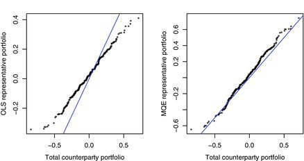
To further showcase the improvement of MQE matching over OLS, Figure 7 plots the sample quantiles of the representative portfolios ${\widetilde{\mathit{}\mathbf{\beta }}}^{\text{'}}\mathbf{X}$ and ${\widehat{\mathit{}\mathbf{\beta }}}^{\text{'}}\mathbf{X}$ against the sample quantiles of the total counterparty portfolio Y, based on the 300 post-sample points. It shows clearly that the distribution of the representative portfolio based on MQE $\widehat{\mathit{}\mathbf{\beta }}$ provides much more accurate approximation for the distribution of the total counterparty portfolio than that based on the OLS $\widetilde{\mathit{}\mathbf{\beta }}$. For the latter, the discrepancy is alarmingly large at the two tails of the distribution, where matter most for risk management.

Figure 6 Boxplots of rMSE$\left(\widehat{\mathit{}\mathbf{\beta }}\right)$ for matching the lower 30% of the distribution of Y, where n is sample size, p is the dimension of X, and r is the noise-to-signal ratio.

Figure 7 The plots of the sample quantiles of the representative portfolios based on OLS (the left panel) and MQE (the right panel) against the sample quantiles of the total counterparty portfolio. The straight lines mark the diagonal y = x on which the two quantiles are equal. All the quantiles are calculated based on the 300 post-sample points.

8. PORTFOLIO TRACKING

Portfolio tracking refers to a portfolio assembled with securities which mirrors a benchmark index, such as S&P500 or FTSE100 (Jansen and van Dijk 2002, and Dose and Cincotti 2005). Tracking portfolios can be used as the strategies for investment, hedging and risk management for investment, or as macroeconomic forecasting (Lamont 2001).

Let Y be the return of an index to be tracked, X₁, …, X_p be the returns of the p securities to be used for tracking Y. One way to choose a tracking portfolio is to select weights {w_i} to minimize$$\begin{array}{c}\hfill E{\left(Y-\sum _{i=1}^p{w}_i{X}_i\right)}^2\end{array}$$subject to $$\begin{array}{c}\hfill \sum _{i=1}^p{w}_i=1\text{and}\sum _{i=1}^p\left|w_i\right|\le c,\end{array}$$where c ⩾ 1 is a constant. See, for example, Section 3.2 of Fan et al. (2012). In the above expression, w_i is the proportion of the capital invested on the ith security X_i, and w_i < 0 indicates a short sale on X_i. It follows from (8.2$$\begin{array}{c}\hfill \sum _{i=1}^p{w}_i=1\text{and}\sum _{i=1}^p\left|w_i\right|\le c,\end{array}$$) that $$\begin{array}{c}\hfill \sum _{w_i>0}{w}_i\le \frac{1+c}{2},\sum _{w_i<0}\left|w_i\right|\le \frac{c-1}{2}.\end{array}$$Hence, the constant c controls the exposure to short sales. When c = 1, short sales are not permitted.

Instead of using the constrained OLS as in above, one alternative in selecting the tracking portfolio is to match the whole (or a part) of distribution of Y. This leads to a constrained MQE, subject to the constraints in (8.2$$\begin{array}{c}\hfill \sum _{i=1}^p{w}_i=1\text{and}\sum _{i=1}^p\left|w_i\right|\le c,\end{array}$$). Given a set of historical returns {(Y_j, X_j1, …, X_jp), j = 1, …, n}, we use the iterative algorithm in Section 2 to calculate MQE $\widehat{\mathit{}\mathbf{\beta }}$ subject to the constraint $$\begin{array}{c}\hfill \sum _{j=1}^p|{\beta }_j|\le \delta \sum _{i=1}^p\left|{\widehat{\beta }}_i^{\left(0\right)}\right|,\end{array}$$and ${\widehat{\mathit{}\mathbf{\beta }}}^{\left(0\right)}={({\widehat{\beta }}_1^{\left(0\right)},...,{\widehat{\beta }}_p^{\left(0\right)})}^{\text{'}}$ is the unconstrained MQE for β, and δ ∈ (0, 1) is a constant which controls, indirectly, the total exposure to short-sales. This is the standard MQE-LASSO; see (2.12$$\begin{array}{c}\hfill \sum _{i=1}^p\left|{\beta }_i\right|\le C_0,\end{array}$$) in Remark 1(iii) in Section 2. For δ ⩾ 1, $\widehat{\mathit{}\mathbf{\beta }}={\widehat{\mathit{}\mathbf{\beta }}}^{\left(0\right)}$. We transform the constrained MQE $\widehat{\mathit{}\mathbf{\beta }}={({\widehat{\beta }}_1,...,{\widehat{\beta }}_p)}^{\text{'}}$ to the estimates for the proportion weights as follows: $$\begin{array}{c}\hfill {\widehat{w}}_i={\widehat{\beta }}_i/\sum _{1\le j\le n}{\widehat{\beta }}_j,i=1,...,p.\end{array}$$Then $\left\{{\widehat{w}}_i\right\}$ fulfill the constraints in (8.2$$\begin{array}{c}\hfill \sum _{i=1}^p{w}_i=1\text{and}\sum _{i=1}^p\left|w_i\right|\le c,\end{array}$$) with any c satisfying the following condition: $$\begin{array}{c}\hfill c\ge \delta \sum _i\left|{\widehat{\beta }}_i^{\left(0\right)}\right|/\left|\sum _j{\widehat{\beta }}_j\right|.\end{array}$$Such a c is always greater than 1 as $$\begin{array}{c}\hfill \delta \sum _i|{\widehat{\beta }}_i^{\left(0\right)}|/|\sum _j{\widehat{\beta }}_j|\ge \delta \sum _i|{\widehat{\beta }}_i^{\left(0\right)}|/\sum _j\left|{\widehat{\beta }}_j\right|\ge 1,\end{array}$$see (8.4$$\begin{array}{c}\hfill \sum _{j=1}^p|{\beta }_j|\le \delta \sum _{i=1}^p\left|{\widehat{\beta }}_i^{\left(0\right)}\right|,\end{array}$$). Note that the LARS-LASSO algorithm gives the whole solution path for all positive values of δ. Hence for a given value c in (8.2$$\begin{array}{c}\hfill \sum _{i=1}^p{w}_i=1\text{and}\sum _{i=1}^p\left|w_i\right|\le c,\end{array}$$), we can always find the largest possible value δ from the solution path for which (8.5$$\begin{array}{c}\hfill c\ge \delta \sum _i\left|{\widehat{\beta }}_i^{\left(0\right)}\right|/\left|\sum _j{\widehat{\beta }}_j\right|.\end{array}$$) holds.

Table 5 The mean, maximum and minimum daily log returns (in percentages) of FTSE100 and the estimated track portfolios in 2007. The estimation was based on the data in 2004–2006. Also included in the table are the number of stocks present in each portfolio, the standard deviations (STD) and the negative mean (NM) of the daily returns, and the percentages (of the capital) for short sales

Portfolio	No. of		Return				Short
	stocks	Mean	Max	Min	STD	NM	sales
FTSE100	100	0.014	3.444	−4.185	1.100	−0.889	0
OLS	30	0.014	3.532	−3.716	1.094	−0.851	0
MQE	30	0.013	3.552	−3.739	1.098	−0.869	0
OLS-lasso (δ = 0.7)	23	0.021	3.943	−4.300	1.250	−0.965	0
MQE-lasso (δ = 0.7)	21	0.049	4.062	−5.247	1.488	−1.150	0
OLS-lasso (δ = 0.5)	14	0.045	4.011	−4.963	1.415	−1.119	0
MQE-lasso (δ = 0.5)	10	0.119	5.05	−6.196	1.825	−1.336	0
MQE-lasso (δ = 0.7, α1 = 0, α2 = 0.5)	13	0.316	18.51	−8.015	2.805	−1.804	38.4
MQE-lasso (δ = 0.7, α1 = 0.25, α2 = 0.75)	11	−0.040	3.864	−4.715	1.567	−1.233	3.9
MQE-lasso (δ = 0.7, α1 = 0.5, α2 = 1)	15	1.608	52.77	−48.63	15.56	−11.93	885
MQE-lasso (δ = 0.5, α1 = 0, α2 = 0.5)	12	0.223	14.55	−6.936	2.330	−1.563	1.4
MQE-lasso (δ = 0.5, α1 = 0.25, α2 = 0.75)	15	0.077	7.858	−8.866	2.295	−1.743	0
MQE-lasso (δ = 0.5, α1 = 0.5, α2 = 1)	5	−0.036	4.375	−5.776	1.791	−1.119	22.0

Figure 8 The plots of the daily log returns of FTSE100 index (thick black cycles), the MQE-LASSO portfolio with δ = 0.7 (thin red cycle in the top panel), and the MQE-LASSO portfolio with δ = 0.5 and (α₁, α₂) = (0, 0.5) (thin blue cycles in the bottom panel).

Figure 9 The plots of the annual means and standard deviations (STD) of daily log returns of FTSE100 index, the OLS portfolio, the MQE portfolio, the OLS-LASSO portfolio and the MQE-LASSO portfolio in the period of 2007–2013.

Figure 10 The plots of the annual means and standard deviations (STD) of daily log returns of FTSE100 index, and the portfolios based on the MQE-LASSO matching the lower half, the middle half, and the upper half of distribution in the period of 2007–2013.

Remark 5.

One would be tempted to absorb the constraint condition ∑_jw_j = 1 in the estimation directly by letting, for example, $$\begin{array}{c}\hfill Y^{\text{'}}=Y-X_p,X_i^{\text{'}}=X_i-X_p\text{for}1\le i<p.\end{array}$$

Then, one could estimate w₁, …, w_{p − 1} directly by regressing Y′ on X′₁, …, X_{p − 1}′. However, this puts the pth security X_p on a nonequal footing as the other p − 1 securities, which may lead to an adverse effect.

We illustrate our proposal by tracking FTSE100 using 30 actively traded stocks included in FTSE100. The company names and the symbols of those 30 stocks are listed in Appendix II.

We use the log returns (in percentages) calculated using the adjusted daily close prices in 2004–2006 (n = 758) to estimate the tracking portfolios by MQE with or without the LASSO, and compare their performance with the returns of FTSE100 in 2007 (in total 253 trading days). We also include in the comparison the portfolios estimated by OLS. The market is overall bullish in the period 2004–2007. The data were downloaded from Yahoo!Finance.

Table 5 list some summary statistics of the daily log-returns in 2007 of FTSE100 and the various tracking portfolios. Both the OLS and the MQE track well the FTSE100 index with almost identical daily mean 0.014%. In addition to the standard deviations (STD), we also include in the table the negative mean (NM) as a risk measure, which is defined as the mean value of all the negative returns. According to both STD and NM, both the OLS and the MQE are slightly less risky than FTSE100 in 2007.

We also form the portfolios based on OLS-LASSO and MQE-LASSO with the truncated parameter δ = 0.7 and 0.5; see (8.4$$\begin{array}{c}\hfill \sum _{j=1}^p|{\beta }_j|\le \delta \sum _{i=1}^p\left|{\widehat{\beta }}_i^{\left(0\right)}\right|,\end{array}$$). Now all the four portfolios yield noticeably greater average daily returns than that of FTSE100 with noticeably greater risks. Furthermore, the performances of OLS and MQE part from each other with MQE producing substantially larger returns with larger risks. For example, the MQE-LASSO portfolio with δ = 0.5 yields average daily return of 0.119% and NM −1.336% while the OLS-LASSO yields average daily return of 0.045% and NM −1.119%. The number of stocks selected in portfolio is 10 by MQE, and 14 by OLS.

We continue the experiment by using the MQE matching the lower half, the middle half and the upper half of the distribution only; see Remark 1(ii). With δ = 0.7, the portfolios resulted from matching either the lower or the upper half of the distribution incur excessive short sales of, respectively, 38.4% and 885% of the initial capital, and are therefore too risky. By using δ = 0.5, short sales are reduced to 1.4% and 22% respectively. Especially matching the lower half distribution with δ = 0.5 leads to a portfolio with average daily return 0.223%, the STD 2.33%, the NA −1.56% and short sales 1.4%.

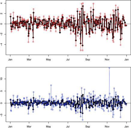
Figure 8 plots the daily returns of FTSE100 together with the two portfolios estimated by the MQE-LASSO with δ = 0.7, and δ = 0.5, (α₀, α₁) = (0, 0.5), respectively. Both the portfolios track well the index with increased volatility. Especially the portfolio plotted in blue is obtained by matching the lower half distribution only. Comparing with FTSE100, the increase of the STD is 1.23% while the increase of the NM is merely 0.654%. The increase of the return for this portfolio is resulted from mimicking the loss of FTSE100 and “freeing” the top half distribution.

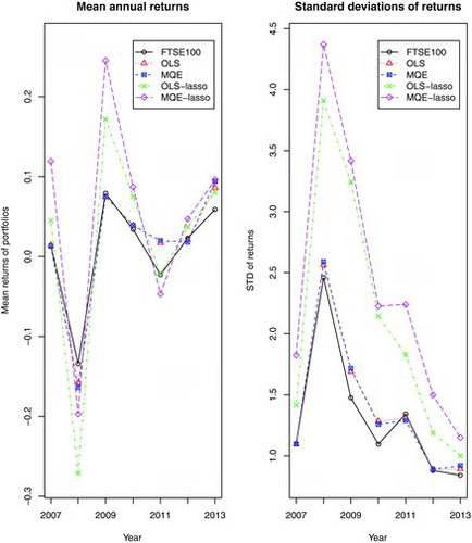
Now we apply the above approach with a rolling window to the data in 2007–2013. More precisely, for each calendar year within the period, we use the data in its previous three years for estimation to form the different portfolios. We then calculate the means and standard deviations for the daily returns in that year based on each of the portfolios. (The data for 2013 were only up to 10 September when this exercise was conducted.) The results for the portfolios based on OLS, MQE with and without LASSO are plotted in Figure 9. We set δ = 0.5 in all the LASSO estimations. Figure 9 shows that the MQE-LASSO portfolio generated greater average returns in the 5 out of 7 years than the other four portfolios. But it also led to greater losses than FTSE100 index in both 2008 and 2011. Judging by the standard deviations it is the most risky strategy among the five portfolios reported in Figure 9. Note that both the OLS and MQE portfolios incur small increases in standard deviation while the gains in average returns in 2011 and 2013 are noticeable. This shows that it is possible to match the overall performance of the index by trading on much fewer stocks.

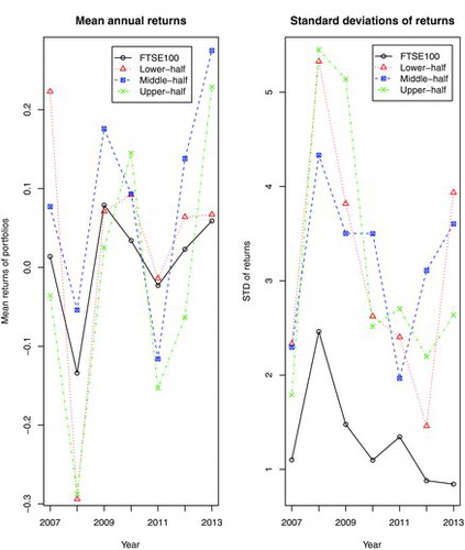
Figure 10 compares the three portfolios based on the MQE-LASSO matching, respectively, the lower half, the middle half and the upper half of the distributions for the returns of FTSE100 index. The first panel in the figure suggests that matching the upper-half distributions leads to very volatile average returns which are worse than the returns of FTSE100 index overall. In contrast, matching the lower half or the middle half of the distributions provide better return than the index in the 6 out of 7 years during the period. The risks of those portfolios, measured by the standard deviations, are higher that those of the index; see the second panel in the figure.

Overall the MQE-LASSO portfolios tend to overshoot at both the peaks and the troughs. Therefore they tend to outperform FTSE100 index when the market is bullish, and they may also do worse than the index when the market is bearish (such as 2008 and 2011).

Additional information

Notes on contributors

Nikolaos Sgouropoulos

Nikolaos Sgouropoulos is Quantitative Analyst, QA Exposure Analytics, Barclays, London, UK (E-mail: [email protected]).

Qiwei Yao

Qiwei Yao is Professor, Department of Statistics, The London School of Economics and Political Science, Houghton Street, London, WC2A 2AE, UK; Guanghua School of Management, Peking University, China (E-mail: [email protected]).

Claudia Yastremiz

Claudia Yastremiz is Senior Technical Specialist, Market and Counterparty Credit Risk Team, Prudential Regulation Authority, Bank of England, London, UK (E-mail: [email protected]).

APPENDIX I: PROOF OF THEOREM 2

We split the proof of Theorem 2 into several lemmas.

Lemma A.1.

Under Conditions B(i) and (ii), n^τ{S_n(β) − S(β)} → 0 in probability for any fixed β and τ < 1/2.

Proof.

Put W = β′X. By (4.7$$\begin{array}{ccc}& & \underset{{\alpha }_1\le \alpha \le {\alpha }_2}{sup}|\sqrt{n}{f}_{{\mathit{}\mathbf{\beta }}^{\text{'}}\mathbf{X}}\left(Q_{{\mathit{}\mathbf{\beta }}^{\text{'}}\mathbf{X}}\left(\alpha \right)\right)\{Q_{n,{\mathit{}\mathbf{\beta }}^{\text{'}}\mathbf{X}}\left(\alpha \right)-Q_{{\mathit{}\mathbf{\beta }}^{\text{'}}\mathbf{X}}\left(\alpha \right)\}\hfill \\ & & +\sqrt{n}\{F_{n,{\mathit{}\mathbf{\beta }}^{\text{'}}\mathbf{X}}\left(Q_{{\mathit{}\mathbf{\beta }}^{\text{'}}\mathbf{X}}\left(\alpha \right)\right)-\alpha \}|\hfill \\ & & =O_P\left(n^{-1/4}{(logn)}^{1/2}{(loglogn)}^{1/4}\right),\hfill \end{array}$$) and (4.8$$\begin{array}{c}\hfill \underset{{\alpha }_1\le \alpha \le {\alpha }_2}{sup}|\sqrt{n}{f}_Y\left(Q_Y\left(\alpha \right)\right)\{Q_{n,Y}\left(\alpha \right)-Q_Y\left(\alpha \right)\}\\ \hfill +\sqrt{n}\{F_{n,Y}\left(Q_Y\left(\alpha \right)\right)-\alpha \}|\\ \hfill =O_P\left(n^{-1/4}{(logn)}^{1/2}{(loglogn)}^{1/4}\right).\end{array}$$), $$\begin{array}{ccc}& & \frac{1}{n}\sum _{j=n_1+1}^{n_2}{\{Q_{n,Y}(j/n)-Q_{n,W}(j/n)\}}^2\hfill \\ & & -\frac{1}{n}\sum _{j=n_1+1}^{n_2}{\{Q_Y(j/n)-Q_W(j/n)\}}^2\hfill \\ & & =\frac{1}{n}\sum _{j=n_1+1}^{n_2}{\left\{\frac{F_{n,Y}\left(Q_Y\left(\alpha \right)\right)-\alpha }{f_Y\left(Q_Y\left(\alpha \right)\right)}\right\}}^2\hfill \\ & & +\frac{1}{n}\sum _{j=n_1+1}^{n_2}{\left\{\frac{F_{n,W}\left(Q_W\left(\alpha \right)\right)-\alpha }{f_W\left(Q_W\left(\alpha \right)\right)}\right\}}^2\hfill \\ & & +\frac{2R_n}{n^{3/2}}\sum _{j=n_1+1}^{n_2}\{Q_Y(j/n)-Q_W(j/n)+F_{n,Y}\left(Q_Y\left(\alpha \right)\right)\hfill \\ & & -\frac{\alpha }{f_Y\left(Q_Y\left(\alpha \right)\right)}-\frac{F_{n,W}\left(Q_W\left(\alpha \right)\right)-\alpha }{f_W\left(Q_W\left(\alpha \right)\right)}\}+O_P(R_n^2/n),\hfill \end{array}$$where R_n = O_P(n^{− 1/4}(log n)^1/2(log log n)^1/4) = o_P(1). By the Dvoretzky-Kiefer-Wolfowitz inequality (Massart 1990), it holds for any constant C > 0 and any integer n ⩾ 1 that $$\begin{array}{c}\hfill P\left\{\underset{0\le \alpha \le 1}{sup}|F_{n,Y}\left(Q_Y\left(\alpha \right)\right)-\alpha |>C\right\}\le 2e^{-2n{C}^2},\\ \hfill P\left\{\underset{0\le \alpha \le 1}{sup}|F_{n,W}\left(Q_W\left(\alpha \right)\right)-\alpha |>C\right\}\le 2e^{-2n{C}^2}.\end{array}$$Let $C=n^{-{\tau }_1}$ for some τ₁ ∈ (τ/2, 1/4), and $$\begin{array}{ccc}& & A_n=\left\{\underset{0\le \alpha \le 1}{sup}|F_{n,Y}\left(Q_Y\left(\alpha \right)\right)-\alpha |\le C\right\}\bigcap \hfill \\ & & \left\{\underset{0\le \alpha \le 1}{sup}|F_{n,W}\left(Q_W\left(\alpha \right)\right)-\alpha |\le C\right\}.\hfill \end{array}$$Then by (A.2$$\begin{array}{c}\hfill P\left\{\underset{0\le \alpha \le 1}{sup}|F_{n,Y}\left(Q_Y\left(\alpha \right)\right)-\alpha |>C\right\}\le 2e^{-2n{C}^2},\\ \hfill P\left\{\underset{0\le \alpha \le 1}{sup}|F_{n,W}\left(Q_W\left(\alpha \right)\right)-\alpha |>C\right\}\le 2e^{-2n{C}^2}.\end{array}$$), $P\left(A_n\right)\ge 1-4e^{-2n{C}^2}\to 1$, and on the set A_n, $$\begin{array}{ccc}& & n^{\tau }\{\frac{1}{n}\sum _{j=n_1+1}^{n_2}{\{Q_{n,Y}(j/n)-Q_{n,W}(j/n)\}}^2\hfill \\ & & -\frac{1}{n}\sum _{j=n_1+1}^{n_2}{\{Q_Y(j/n)-Q_W(j/n)\}}^2\}=o_P\left(1\right),\hfill \end{array}$$which is guaranteed by Condition B(ii) and the fact that $$\begin{array}{c}\hfill \frac{1}{n}\sum _{j=n_1+1}^{n_2}\left\{Q_Y(j/n)-Q_W(j/n)\right\}\to {\int }_{{\alpha }_1}^{{\alpha }_2}\{Q_Y\left(\alpha \right)-Q_W\left(\alpha \right)\}d\alpha .\end{array}$$Note that $$\begin{array}{c}\hfill \left|{\int }_{{\alpha }_1}^{{\alpha }_2}\right\{Q_Y\left(\alpha \right)-Q_W\left(\alpha \right)\left\}d\alpha \right|\le {\int }_{{\alpha }_1}^{{\alpha }_2}\left\{|Q_Y\left(\alpha \right)|+|Q_W\left(\alpha \right)|\right\}d\alpha \\ \hfill =E\left[\right|Y\left|I\{G_Y\left({\alpha }_1\right)<Y\le G_Y\left({\alpha }_2\right)\}\right]+E\left|W\right|<\infty ,\end{array}$$as |Y|I{G_Y(α₁) < Y ⩽ G_Y(α₂)} is bounded under Condition B(ii). See also condition B(iii) and Remark 3(iii).

Under Condition B(ii), |Q_Y(α) − Q_Y(j/n)| = f_Y(j/n)^{− 1}/n{1 + o(1)} for any |α − j/n| ⩽ 1/n. Hence $$\begin{array}{ccc}& & \frac{1}{n}\sum _{j=n_1+1}^{n_2}{\{Q_Y(j/n)-Q_W(j/n)\}}^2\hfill \\ & & ={\int }_{{\alpha }_1}^{{\alpha }_2}{\{Q_Y\left(\alpha \right)-Q_W\left(\alpha \right)\}}^{2}d\alpha +o(1/n).\hfill \end{array}$$Combining this with (A.3$$\begin{array}{ccc}& & n^{\tau }\{\frac{1}{n}\sum _{j=n_1+1}^{n_2}{\{Q_{n,Y}(j/n)-Q_{n,W}(j/n)\}}^2\hfill \\ & & -\frac{1}{n}\sum _{j=n_1+1}^{n_2}{\{Q_Y(j/n)-Q_W(j/n)\}}^2\}=o_P\left(1\right),\hfill \end{array}$$), we obtain the required result.

Lemma A.2.

Let a₁ ⩽ ⋅⋅⋅ ⩽ a_n be n real numbers. Let b_i = a_i + δ_i for i = 1, …, n, and δ_i are real numbers. Then$$\begin{array}{c}\hfill \underset{1\le i\le n}{max}|a_i-b_{\left(i\right)}|\le \underset{1\le j\le n}{max}\left|{\delta }_j\right|,\end{array}$$where b₍₁₎ ⩽ ⋅⋅⋅ ⩽ b_(n) is a permutation of {b₁, …, b_n}.

Proof.

We use the mathematical induction to prove the lemma. Let ε = max _j|δ_j|. It is easy to see that (A.4$$\begin{array}{c}\hfill \underset{1\le i\le n}{max}|a_i-b_{\left(i\right)}|\le \underset{1\le j\le n}{max}\left|{\delta }_j\right|,\end{array}$$) is true for n = 2. Let it be also true for n = k. We now prove it for n = k + 1.

Let c_i = b_i for i = 1, …, k. Then by the induction assumption,$$\begin{array}{c}\hfill \underset{1\le i\le k}{max}|a_i-c_{\left(i\right)}|\le ϵ.\end{array}$$If b_{k + 1} = a_{k + 1} + δ_{k + 1} ⩾ c_(k), the required result holds. However, if for some 1 ⩽ i < k, $$\begin{array}{c}\hfill c_{\left(i\right)}\le b_{k+1}<c_{(i+1)},\end{array}$$then $$\begin{array}{c}\hfill b_{\left(j\right)}=\left\{\begin{array}{cc}{c}_{\left(j\right)}\hfill & 1\le j\le i,\hfill \\ b_{k+1}\hfill & j=i+1,\hfill \\ c_{(j-1)}\hfill & i+2\le j\le k+1.\hfill \end{array}\right.\end{array}$$

Note that |b_{k + 1} − a_{i + 1}| ⩽ ε since $$\begin{array}{c}\hfill b_{k+1}=a_{k+1}+{\delta }_{k+1}\ge a_{i+1}-ϵ\text{and}{b}_{k+1}<c_{(i+1)}\le a_{i+1}+ϵ.\end{array}$$The second expression above is implied by (A.5$$\begin{array}{c}\hfill \underset{1\le i\le k}{max}|a_i-c_{\left(i\right)}|\le ϵ.\end{array}$$).

On the other hand, for j = i + 2, …, k + 1, we need to show that |c_{(j − 1)} − a_j| ⩽ ε. This is true, as c_{(j − 1)} ⩽ a_{j − 1} + ε ⩽ a_j + ε, and furthermore $$\begin{array}{c}\hfill c_{(j-1)}>b_{k+1}=a_{k+1}+{\delta }_{k+1}\ge a_j-ϵ.\end{array}$$Hence |b_(j) − a_j| ⩽ ε for all 1 ⩽ j ⩽ k + 1. This completes the proof.

Lemma A.3.

Let Condition B hold. Let $\mathcal{B}$ be any compact subset of R^p. It holds that ${sup}_{\mathit{}\mathbf{\beta }\in \mathcal{B}}|S_n\left(\mathit{}\mathbf{\beta }\right)-S\left(\mathit{}\mathbf{\beta }\right)|$ converges to 0 in probability.

Proof.

We denote by ||β|| the Euclidean norm of vector β, and |β| = ∑_j|β_j|. Note that S(β) is a continuous function in β. For any ε > 0, there exist ${\mathit{}\mathbf{\beta }}_1,...,{\mathit{}\mathbf{\beta }}_m\in \mathcal{B}$, where m is finite, such that for any $\mathit{}\mathbf{\beta }\in \mathcal{B}$, there exists 1 ⩽ i ⩽ m for which $$\begin{array}{c}\hfill \left|\right|\mathit{}\mathbf{\beta }-{\mathit{}\mathbf{\beta }}_i\left|\right|<ϵ/max(M,\sqrt{p})\text{and}|S\left(\mathit{}\mathbf{\beta }\right)-S\left({\mathit{}\mathbf{\beta }}_i\right)|<ϵ,\end{array}$$where M > 0 is a constant such that ||x|| < M for any f_X(x) > 0; see Condition B(iii). Thus $$\begin{array}{ccc}& & |{\mathit{}\mathbf{\beta }}^{\text{'}}\mathbf{x}-{\mathit{}\mathbf{\beta }}_i^{\text{'}}\mathbf{x}|\le |\left|\mathbf{x}\right||·||\mathit{}\mathbf{\beta }-{\mathit{}\mathbf{\beta }}_i\left|\right|\le ϵ,\left|\right|\mathit{}\mathbf{\beta }|-|{\mathit{}\mathbf{\beta }}_i\left|\right|\le |\mathit{}\mathbf{\beta }-{\mathit{}\mathbf{\beta }}_i|\hfill \\ & & \le \sqrt{p}\left|\right|\mathit{}\mathbf{\beta }-{\mathit{}\mathbf{\beta }}_i\left|\right|\le ϵ.\hfill \end{array}$$Now it follows from Lemma A.2 that $$\begin{array}{ccc}& & |S_n\left(\mathit{}\mathbf{\beta }\right)-S_n\left({\mathit{}\mathbf{\beta }}_i\right)|\le \frac{1}{n}\sum _{j=n_1+1}^{n_2}{\left\{{\left({\mathit{}\mathbf{\beta }}_i^{\text{'}}\mathbf{X}\right)}_{\left(j\right)}-{\left({\mathit{}\mathbf{\beta }}^{\text{'}}\mathbf{X}\right)}_{\left(j\right)}\right\}}^2\hfill \\ & & +\frac{2}{n}\sum _{j=n_1+1}^{n_2}|{\left({\mathit{}\mathbf{\beta }}_i^{\text{'}}\mathbf{X}\right)}_{\left(j\right)}-{\left({\mathit{}\mathbf{\beta }}^{\text{'}}\mathbf{X}\right)}_{\left(j\right)}||Y_{\left(j\right)}-{\left({\mathit{}\mathbf{\beta }}_i^{\text{'}}\mathbf{X}\right)}_{\left(j\right)}|\hfill \\ & & +\left|\right|\mathit{}\mathbf{\beta }|-|{\mathit{}\mathbf{\beta }}_i\left|\right|\le {ϵ}^2+ϵ\frac{2}{n}\sum _{j=n_1+1}^{n_2}|Y_{\left(j\right)}-{\left({\mathit{}\mathbf{\beta }}_i^{\text{'}}\mathbf{X}\right)}_{\left(j\right)}|\hfill \\ & & +ϵ\to {ϵ}^2+2ϵ{\int }_{{\alpha }_1}^{{\alpha }_2}|G_Y\left(\alpha \right)-G_{{\mathit{}\mathbf{\beta }}_i^{\text{'}}X}\left(\alpha \right)|d\alpha +ϵ\hfill \end{array}$$

in probability. This limit can be verified in the similar manner as in the proof of Lemma A.1. Consequently, there exists a set A with P(A) ⩾ 1 − ε such that on the set A it holds that $$\begin{array}{c}\hfill |S_n\left(\mathit{}\mathbf{\beta }\right)-S_n\left({\mathit{}\mathbf{\beta }}_i\right)|\le ϵC,\end{array}$$where C > 0 is a constant. Now on the set A, $$\begin{array}{ccc}& & |S_n\left(\mathit{}\mathbf{\beta }\right)-S\left(\mathit{}\mathbf{\beta }\right)|\le |S_n\left(\mathit{}\mathbf{\beta }\right)-S_n\left({\mathit{}\mathbf{\beta }}_i\right)|\hfill \\ & & +|S_n\left({\mathit{}\mathbf{\beta }}_i\right)-S\left({\mathit{}\mathbf{\beta }}_i\right)|+|S\left({\mathit{}\mathbf{\beta }}_i\right)-S\left(\mathit{}\mathbf{\beta }\right)|\hfill \\ & & \le ϵC+|S_n\left({\mathit{}\mathbf{\beta }}_i\right)-S\left({\mathit{}\mathbf{\beta }}_i\right)|+ϵ.\hfill \end{array}$$See (A.6$$\begin{array}{c}\hfill \left|\right|\mathit{}\mathbf{\beta }-{\mathit{}\mathbf{\beta }}_i\left|\right|<ϵ/max(M,\sqrt{p})\text{and}|S\left(\mathit{}\mathbf{\beta }\right)-S\left({\mathit{}\mathbf{\beta }}_i\right)|<ϵ,\end{array}$$). Hence it holds on the set A that $$\begin{array}{c}\hfill \underset{\mathit{}\mathbf{\beta }\in \mathcal{B}}{sup}|S_n\left(\mathit{}\mathbf{\beta }\right)-S\left(\mathit{}\mathbf{\beta }\right)|\le ϵ(C+1)+\sum _{i=1}^m|S_n\left({\mathit{}\mathbf{\beta }}_i\right)-S\left({\mathit{}\mathbf{\beta }}_i\right)|.\end{array}$$Now the required convergence follows from Lemma A.1.

Proof of Theorem 2.

Under Condition B(ii), YI{Q_Y(α₁) ⩽ Y ⩽ Q_Y(α₂)} is bounded. As X is also bounded, the MQE $\widehat{\mathit{}\mathbf{\beta }}$ defined in (4.2$$\begin{array}{c}\hfill \widehat{\mathit{}\mathbf{\beta }}=arg\underset{\mathit{}\mathbf{\beta }}{min}{S}_n\left(\mathit{}\mathbf{\beta }\right),\end{array}$$) is also bounded. Let $\mathcal{B}$ be a compact set which contains $\widehat{\mathit{}\mathbf{\beta }}$ with probability 1.

By (4.1$$\begin{array}{ccc}\hfill {\mathit{}\mathbf{\beta }}_0& =& arg\underset{\mathit{}\mathbf{\beta }}{min}S\left(\mathit{}\mathbf{\beta }\right),S\left(\mathit{}\mathbf{\beta }\right)\equiv S(\mathit{}\mathbf{\beta };{\alpha }_1,{\alpha }_2)\hfill \\ & =& {\int }_{{\alpha }_1}^{{\alpha }_2}{\{Q_Y\left(\alpha \right)-Q_{{\mathit{}\mathbf{\beta }}^{\text{'}}\mathbf{X}}\left(\alpha \right)\}}^{2}d\alpha +\lambda \sum _{j=1}^p\left|{\beta }_j\right|.\hfill \end{array}$$) and (4.2$$\begin{array}{c}\hfill \widehat{\mathit{}\mathbf{\beta }}=arg\underset{\mathit{}\mathbf{\beta }}{min}{S}_n\left(\mathit{}\mathbf{\beta }\right),\end{array}$$), $$\begin{array}{c}\hfill S_n\left({\mathit{}\mathbf{\beta }}_0\right)-S\left({\mathit{}\mathbf{\beta }}_0\right)\ge S_n\left(\widehat{\mathit{}\mathbf{\beta }}\right)-S\left({\mathit{}\mathbf{\beta }}_0\right)\ge S_n\left(\widehat{\mathit{}\mathbf{\beta }}\right)-S\left(\widehat{\mathit{}\mathbf{\beta }}\right).\end{array}$$Now it follows from Lemma A.3 that both S_n(β₀) − S(β₀) and $S_n\left(\widehat{\mathit{}\mathbf{\beta }}\right)-S\left(\widehat{\mathit{}\mathbf{\beta }}\right)$ converge to 0 in probability. Hence, $S_n\left(\widehat{\mathit{}\mathbf{\beta }}\right)-S\left({\mathit{}\mathbf{\beta }}_0\right)$ also converges to 0 in probability.

For the second assertion, we need to prove that $P\{d({\widehat{\mathit{}\mathbf{\beta }}}_n,{\mathcal{B}}_0)\ge ϵ\}\to 0$ for any constant ϵ > 0. We now write ${\widehat{\mathit{}\mathbf{\beta }}}_n=\widehat{\mathit{}\mathbf{\beta }}$ to indicate explicitly that the estimator is defined with the sample of size n. We proceed by contradiction. Suppose there exists an ϵ > 0 for which $$\begin{array}{c}\hfill \underset{n\to \infty }{lim\; sup}P\{d(\widehat{\mathit{}\mathbf{\beta }},{\mathcal{B}}_0)\ge ϵ\}>0.\end{array}$$Hence, there exists an integer subsequence n_k such that lim_kP(A_k) = δ > 0, where A_k is defined as $$\begin{array}{c}\hfill A_k=\{d({\widehat{\mathit{}\mathbf{\beta }}}_{n_k},{\mathcal{B}}_0)\ge ϵ\}.\end{array}$$Let ${\mathcal{B}}_1=\{\mathit{}\mathbf{\beta }\in \mathcal{B}:d(\mathit{}\mathbf{\beta },{\mathcal{B}}_0)\ge ϵ\}$. Then ${\mathcal{B}}_1$ is a compact set which is ϵ-distance away from ${\mathcal{B}}_0$. By the definition of ${\mathcal{B}}_0$ in (4.4$$\begin{array}{c}\hfill {\mathcal{B}}_0=\{\mathit{}\mathbf{\beta }:S\left(\mathit{}\mathbf{\beta }\right)=S\left({\mathit{}\mathbf{\beta }}_0\right)\},\end{array}$$), $$\begin{array}{c}\hfill \underset{\mathit{}\mathbf{\beta }\in {\mathcal{B}}_1}{inf}S\left(\mathit{}\mathbf{\beta }\right)=\delta +S\left({\mathit{}\mathbf{\beta }}_0\right).\end{array}$$where δ > 0 is a constant. By Lemma A.3, P(B_k) → 1 for $$\begin{array}{c}\hfill B_k=\left\{\right|S_{n_k}\left({\widehat{\mathit{}\mathbf{\beta }}}_{n_k}\right)-S\left({\widehat{\mathit{}\mathbf{\beta }}}_{n_k}\right)|<\delta /2\}.\end{array}$$Now it holds on the set A_k∩B_k that $$\begin{array}{c}\hfill S_{n_k}\left({\widehat{\mathit{}\mathbf{\beta }}}_{n_k}\right)\ge S\left({\widehat{\mathit{}\mathbf{\beta }}}_{n_k}\right)-\delta /2\ge \underset{\mathit{}\mathbf{\beta }\in {\mathcal{B}}_1}{inf}S\left(\mathit{}\mathbf{\beta }\right)-\delta /2>S\left({\mathit{}\mathbf{\beta }}_0\right)+\delta /2>S\left({\mathit{}\mathbf{\beta }}_0\right).\end{array}$$This contradicts to the fact that $S_n\left(\widehat{\mathit{}\mathbf{\beta }}\right)$ converges to S(β₀) in probability, which was established earlier. This completes the proof.$\square$

ACKNOWLEDGMENTS

We thank Professor Wolfgang Polonik for his helpful comments, in particular for drawing our attention to references Kiefer (1970) and Kulik (2007). We also thank the Editor and three reviewers for their critical and helpful comments and suggestions.

APPENDIX II: THE NAMES OF SYMBOLS OF THE 30 STOCKS USED IN TRACKING FTSE100

 

Table

ANTO	Antofagasta	CRDA	Croda International	OML	Old Mutual
ARM	ARM Holdings	DGE	Diageo	PRU	Prudential
BARC	Barclays	GSK	GlaxoSmith Kline	RBS	Royal Bank of Scotland
BATS	British American Tobacco	HSBA	HSBC Holdings	RDSB	Royal Dutch Shell
BG	BG Group	ITV	ITV	RIO	Rio Tinto
BLT	BHP Billiton	LGEN	Legal & General Group	RR	Rolls-Royce Group
BP	BP	LLOY	Lloyds Banking Group	RSA	RSA Insurance Group
BSY	British Sky Broadcasting	MKS	Marks & Spencer Group	TSCO	Tesco
BT-A	BT Group	MRW	Morrison Supermarkets	ULVR	Unilever
CNA	Centrica	NG	National Grid	VOD	Vodafone Group

REFERENCES

- An, H.-Z., Huang, D., Yao, Q., and Zhang, C.-H. (2008), “Stepwise Searching for Feature Variables in High-dimensional Linear Regression,” unpublished manuscript, available at http://stats.lse.ac.uk/q.yao/qyao.links/paper/ahyz08.pdf.
- Bickel, P.J., and Freedman, D.A. (1981), “Some Asymptotic Theory for the Bootstrap,” The Annals of Statistics, 9, 1196–1217.
- del Barrio, E., Cuesta-Albertos, J.A., Matrán, C., and Rodríguez-Rodríguez, J.M. (1999), “Tests of Goodness of Fit Based on the-Wasserstein Distance L2,” The Annals of Statistics, 27, 1230–1239.
- Dominicy, Y., and Veredas, D. (2013), “The Method of Simulated Quantiles,” Journal of Econometrics, 172, 208–221.
- Dose, C., and Cincotti, S. (2005), “Clustering of Financial Time Series with Application to Index and Enhanced Index Tracking Portfolio,” Physica A, 355, 145–151.
- Efron, B., Johnstone, I., Hastie, T., and Tibshirani, R. (2004), “Least Angle Regression” (with discussions), The Annals of Statistics, 32, 409–499.
- Fan, J., Zhang, J., and Yu, K. (2012), “Vast Portfolio Selection with Gross-exposure Constraints,” Journal of the American Statistical Association, 107, 592–606.
- Firpo, S., Fortin, N., and Lemieux, T. (2009), “Unconditional Quantile Regressions,” Econometrica, 77, 953–973.
- Gneiting, T. (2011), “Quantiles as Optimal Point Forecasts,” International Journal of Forecasting, 27, 197–207.
- He, X., Yang, Y., and Zhang, J. (2012), “Bivariate Downscaling with Asynchronous Measurements,” Journal of Agricultural, Biological, and Environmental Statistics, 17, 476–489.
- Jansen, R. and van Dijk, R. (2002), “Optimal Benchmark Tracking with Small Portfolios,” The Journal of Portfolio Management, 28, 33–39.
- Karian, Z., and Dudewicz, E. (1999), “Fitting the Generalized Lambda Distribution to Data: A Method Based on Percentiles,” Communications in Statistics: Simulation and Computation, 28, 793–819.
- Kiefer, J. (1970), “Deviations Between the Sample Quantile Process and the Sample DF,” in Nonparametric Techniques in Statistical Inference ed. M. L. Puri, pp. 299–319, London: Cambridge University Press.
- Koenker, R. (2005), Quantile Regression, Cambridge: Cambridge University Press.
- Kosorok, M.R. (1999), “Two-Sample Quantile Tests Under General Conditions,” Biometrika, 86, 909–921.
- Kulik, R. (2007), “Bahadur-Kiefer Tample Quantiles of Weakly Dependent Linear Processes,” Bernoulli, 13, 1071–1090.
- Lamont, O.A. (2001), “Economic Tracking Portfolios,” Journal of Econometrics, 105, 161–184.
- Mallows, C.L. (1972), “A Note on Asymptotic Joint Normality,” The Annals of Mathematical Statistics, 43, 508–515.
- Massart, P. (1990), “The Tight Constant in the Dvoretzky-Kiefer-Wolfowitz Inequality,” The Annals of Probability, 18, 1269–1283.
- O’Brien, T.P., Sornette, D., and McPherro, R.L. (2001), “Statistical Asynchronous Regression Determining: The Relationship Between Two Quantities that are not Measured Simultaneously,” Journal of Geophysical Research, 106, 13247–13259.
- Serfling, R.J. (1980), Approximation Theorems of Mathematical Statistics, New York: Wiley.
- Small, C., and McLeish, D. (1994), Hilbert Space Methods in Probability and Statistical Inference, New York: Wiley.
- Tanaka, H. (1973), “An Inequality for a Functional of Probability Distribution and its Application to Kac’s One-Dimensional Model of a Maxwellian Gas,” Zeitschrift für Wahrscheinlichkeitstheorie und verwandte Gebiete, 27, 47–52.
- Wu, C. F.J. (1983), “On the Convergence Properties of the EM Algorithm,” The Annals of Statistics, 11, 95–103.