Robust Maximum Association Estimators

ABSTRACT

The maximum association between two multivariate variables $\mathbf{X}$ and $\mathbf{Y}$ is defined as the maximal value that a bivariate association measure between one-dimensional projections ${\alpha }^t\mathbf{X}$ and ${\beta }^t\mathbf{Y}$ can attain. Taking the Pearson correlation as projection index results in the first canonical correlation coefficient. We propose to use more robust association measures, such as Spearman’s or Kendall’s rank correlation, or association measures derived from bivariate scatter matrices. We study the robustness of the proposed maximum association measures and the corresponding estimators of the coefficients yielding the maximum association. In the important special case of $\mathbf{Y}$ being univariate, maximum rank correlation estimators yield regression estimators that are invariant against monotonic transformations of the response. We obtain asymptotic variances for this special case. It turns out that maximum rank correlation estimators combine good efficiency and robustness properties. Simulations and a real data example illustrate the robustness and the power for handling nonlinear relationships of these estimators. Supplementary materials for this article are available online.

KEYWORDS:

• Influence function
• Projection pursuit
• Rank correlation
• Regression
• Robustness

1. Introduction

Association between two univariate variables U and V can be measured in several ways. The correlation coefficients of Pearson, Spearman, and Kendall are standard tools in statistical practice. For measuring the degree of association between two multivariate variables $\mathbf{X}$ and $\mathbf{Y}$, much less literature is existing. An overview of earlier work is given in Ramsay, Ten Berge, and Styan (1984). Recently, Smilde et al. (2009) proposed a matrix association measure for high-dimensional datasets motivated by applications in biology. Nevertheless, the association measures discussed in those articles are based on condensing information from the full covariance matrices and are not very intuitive.

We introduce a class of measures of association between multivariate variables based on the idea of projection pursuit. Suppose that $\mathbf{X}$ is a p-dimensional random vector and $\mathbf{Y}$ is a q-dimensional random vector, with p ⩾ q. A measure of multivariate association between $\mathbf{X}$ and $\mathbf{Y}$ can be defined by looking for linear combinations ${\alpha }^t\mathbf{X}$ and ${\beta }^t\mathbf{Y}$ of the original variables having maximal association. Expressed in mathematical terms, we seek a measure (1) $$\begin{array}{c}\hfill {\rho }_R(\mathbf{X},\mathbf{Y})=\underset{\alpha ,\beta }{max}R({\alpha }^t\mathbf{X},{\beta }^t\mathbf{Y}),\end{array}$$(1) where R is a measure of association between univariate variables. Using the projection pursuit terminology, R is the projection index to maximize. Depending on the choice of R used in the above definition, different measures of association between $\mathbf{X}$ and $\mathbf{Y}$ are obtained. Taking the classical Pearson correlation for R results in the first canonical correlation coefficient (see, e.g., Johnson and Wichern 2002). Other choices of R yield measures ρ_R having different properties. The bivariate association measures considered in this article are Spearman’s rank correlation, Kendall’s τ, and an M-estimator (Huber 1981).

For identifying the vectors $\alpha \in {\mathbb{R}}^p$ and $\beta \in {\mathbb{R}}^q$ in (1(1) $$\begin{array}{c}\hfill {\rho }_R(\mathbf{X},\mathbf{Y})=\underset{\alpha ,\beta }{max}R({\alpha }^t\mathbf{X},{\beta }^t\mathbf{Y}),\end{array}$$(1) ), we impose a unit norm restriction such that (2) $$\begin{array}{c}\hfill ({\alpha }_R(\mathbf{X},\mathbf{Y}),{\beta }_R(\mathbf{X},\mathbf{Y}))=\underset{\parallel \alpha \parallel =1,\parallel \beta \parallel =1}{\text{argmax}}R({\alpha }^t\mathbf{X},{\beta }^t\mathbf{Y}).\end{array}$$(2) We refer to ${\alpha }_R$ and ${\beta }_R$ as the weighting vectors. They indicate the contribution of every single component of $\mathbf{X}$ and $\mathbf{Y}$ in the construction of the linear combinations ${{\alpha }_R}^t\mathbf{X}$ and ${{\beta }_R}^t\mathbf{Y}$ yielding maximal association. This article studies the robustness and efficiency of the maximum association estimators defined in (1(1) $$\begin{array}{c}\hfill {\rho }_R(\mathbf{X},\mathbf{Y})=\underset{\alpha ,\beta }{max}R({\alpha }^t\mathbf{X},{\beta }^t\mathbf{Y}),\end{array}$$(1) ) and (2(2) $$\begin{array}{c}\hfill ({\alpha }_R(\mathbf{X},\mathbf{Y}),{\beta }_R(\mathbf{X},\mathbf{Y}))=\underset{\parallel \alpha \parallel =1,\parallel \beta \parallel =1}{\text{argmax}}R({\alpha }^t\mathbf{X},{\beta }^t\mathbf{Y}).\end{array}$$(2) ).

An important special case is given for univariate Y, where the weighting vector ${\alpha }_R$ can be viewed as a normalized coefficient vector in a linear regression model. Using a rank correlation measure R gives an ${\alpha }_R$ invariant against monotonic transformations of Y. Consider the regression model (3) $$\begin{array}{c}\hfill F\left(Y\right)={\mathbf{a}}^t\mathbf{X}+e,\end{array}$$(3) where F is an unspecified strictly monotonic function and e is a random error term. Han (1987) used the Kendall correlation and proved that the resulting estimator yields consistent estimates of the normalized regression coefficients in (3(3) $$\begin{array}{c}\hfill F\left(Y\right)={\mathbf{a}}^t\mathbf{X}+e,\end{array}$$(3) ). Furthermore, asymptotic normality of this estimator was shown by Sherman (1993). Nevertheless, those authors only consider the Kendall correlation and do not study robustness.

A related, but different concept is that of maximal correlation. There the aim is to find optimal measurable transformations of the variables in $\mathbf{X}$ and $\mathbf{Y}$ such that the first canonical correlation coefficient is maximized. This problem is already relevant and nontrivial for p = q = 1, where one searches measurable functions F and G such that the Pearson correlation between F(X) and G(Y) is maximal. See Papadatos and Xifara (2013) and López Blázquez and Salamanca Miño (2014) for recent references. If (X, Y) follows a bivariate normal distribution, the maximal correlation equals the absolute value of the Pearson correlation (see Yu 2008, for an elegant proof). For p > q = 1, this problem was addressed by Breiman and Friedman (1985), who proposed an algorithm for finding optimal transformations for multiple least-square regression. The general case of both p > 1 and q > 1 does not seem to have received much attention in the statistical literature. The maximum association measure we define in (1(1) $$\begin{array}{c}\hfill {\rho }_R(\mathbf{X},\mathbf{Y})=\underset{\alpha ,\beta }{max}R({\alpha }^t\mathbf{X},{\beta }^t\mathbf{Y}),\end{array}$$(1) ) is different from maximal correlation, since (i) we search for optimal linear combinations of the measured variables without transforming them, and (ii) we gain robustness by taking other choices for R than the Pearson correlation coefficient.

We emphasize that we propose a measure of multivariate association, not a measure of dependence. For instance, if there is perfect association between one component of $\mathbf{X}$ and one component of $\mathbf{Y}$, there is also a perfect multivariate association, even if the other components are independent of each other (see Example 1 of the supplementary report Alfons, Croux, and Filzmoser 2016, p. 1). This should not necessarily be seen as a disadvantage of the proposed measure, as we aim at finding linear projections of multivariate random vectors that are highly associated with each other. In addition, ${\rho }_R(\mathbf{X},\mathbf{Y})=0$ does not imply independence of $\mathbf{X}$ and $\mathbf{Y}$ (see Example 2 of the supplementary report Alfons, Croux, and Filzmoser 2016, p. 1). For comparison, the standard Pearson correlation measure is not sufficient as an index of independence either (for nonnormal distributions), since zero correlation does not imply independence. The projection pursuit approach that we follow is convenient, but not sufficient for describing the full set of possible dependencies. We provide a one-number summary—together with weighting vectors—of the most important association between linear projections of two sets of random variables.

This article studies a multivariate association measure and is not aiming to provide a fully robustified version of canonical correlation analysis (CCA). Note that several articles on robust CCA can be found in the literature. One stream of research is devoted to robustly estimating the covariance matrices involved in solving the CCA problem and investigating the properties of this approach (e.g., Taskinen et al. 2006). Robust estimators for the multivariate linear model are considered in Kudraszow and Maronna (2011) to obtain robust canonical coordinates. A robust alternating regression technique has been used in Branco et al. (2005). They also used a projection pursuit-based algorithm to estimate the canonical variates, and they compared the different approaches by means of simulation studies.

In this article, we go much further and study the theoretical robustness properties of the estimators. In addition, we emphasize on the special case of regression, where asymptotic variances are computed. As a further contribution, we use an extension of the grid algorithm, which was developed by Croux, Filzmoser, and Oliveira (2007) for projection pursuit principal component analysis. A fast implementation of this algorithm is made available for the statistical computing environment R in package ccaPP.

2. Definitions and Basic Properties

Denote R the projection index to be maximized in (1(1) $$\begin{array}{c}\hfill {\rho }_R(\mathbf{X},\mathbf{Y})=\underset{\alpha ,\beta }{max}R({\alpha }^t\mathbf{X},{\beta }^t\mathbf{Y}),\end{array}$$(1) ). The association measure R should verify the following properties, where (U, V) stands for any pair of univariate random variables:

(i)	R(U, V) = R(V, U)
(ii)	$R(aU+b,cV+d)=\text{sign}\left(ac\right)R(U,V)$ for all $a,b,c,d\in \mathbb{R}$
(iii)	− 1 ⩽ R ⩽ 1

Note that condition (ii) gives R( − U, V) = −R(U, V), therefore the proposed measure defined in (1(1) $$\begin{array}{c}\hfill {\rho }_R(\mathbf{X},\mathbf{Y})=\underset{\alpha ,\beta }{max}R({\alpha }^t\mathbf{X},{\beta }^t\mathbf{Y}),\end{array}$$(1) ) verifies ρ_R ⩾ 0. If (U, V) follows a distribution F, we denote R(F) ≡ R(U, V).

The equivariance property (ii) ensures the association measures to be invariant under affine transformations. Indeed, for any nonsingular matrices $\mathbf{A}$ and $\mathbf{B}$ and vectors $\mathbf{a}$ and $\mathbf{b}$, it holds that $$\begin{array}{c}\hfill {\rho }_R(\mathbf{A}\mathbf{X}+\mathbf{a},\mathbf{B}\mathbf{Y}+\mathbf{b})={\rho }_R(\mathbf{X},\mathbf{Y}).\end{array}$$The weighting vectors are affine equivariant in the sense that $$\begin{array}{c}\hfill {\alpha }_R(\mathbf{A}\mathbf{X}+\mathbf{a},\mathbf{B}\mathbf{Y}+\mathbf{b})={\left({\mathbf{A}}^t\right)}^{-1}{\alpha }_R(\mathbf{X},\mathbf{Y})/\parallel {\left({\mathbf{A}}^t\right)}^{-1}{\alpha }_R(\mathbf{X},\mathbf{Y})\parallel \end{array}$$and similarly for ${\beta }_R$. Now we briefly review the definitions of several bivariate association measures R.

2.1. Pearson Correlation

This classical measure for linear association is defined as (4) $$\begin{array}{c}\hfill R_P(U,V)=\frac{\text{cov}\left(U,V\right)}{\sqrt{\text{var}\left(U\right)\text{var}\left(V\right)}}.\end{array}$$(4) The maximization problem in (1(1) $$\begin{array}{c}\hfill {\rho }_R(\mathbf{X},\mathbf{Y})=\underset{\alpha ,\beta }{max}R({\alpha }^t\mathbf{X},{\beta }^t\mathbf{Y}),\end{array}$$(1) ) can now be solved explicitly, since it corresponds to the definition of the first canonical correlation coefficient. We have that ${\rho }_{R_P}$ is given by the square root of the largest eigenvalue of the matrix (5) $$\begin{array}{c}\hfill {\Sigma }_{XX}^{-1}{\Sigma }_{XY}{\Sigma }_{YY}^{-1}{\Sigma }_{YX},\end{array}$$(5) where ${\Sigma }_{XX}=\text{cov}\left(\mathbf{X}\right),{\Sigma }_{YY}=\text{cov}\left(\mathbf{Y}\right)$, ${\Sigma }_{XY}=\text{cov}(\mathbf{X},\mathbf{Y})$, and ${\Sigma }_{YX}={{\Sigma }_{XY}}^t$. Existence of ${\rho }_{R_P}$ requires existence of second moments, while the other measures to be discussed do not require any existence of moments.

We do not aim at constructing robust maximum association measures by plugging robust scatter matrices into (5(5) $$\begin{array}{c}\hfill {\Sigma }_{XX}^{-1}{\Sigma }_{XY}{\Sigma }_{YY}^{-1}{\Sigma }_{YX},\end{array}$$(5) ). The projection pursuit approach that we follow does not require to compute the full scatter matrices and can also be applied if the number of variables in any of the two datasets exceeds the number of observations. However, this article is not focused on such high-dimensional applications.

2.2. Spearman and Kendall Correlation

These well-known measures are based on ranks and signs. The Spearman rank correlation is defined as $$\begin{array}{c}\hfill R_S(U,V)=R_P(\text{rank}\left(U\right),\text{rank}\left(V\right)),\end{array}$$where $\text{rank}\left(u\right)=F_U\left(u\right)$, with F_U the cumulative distribution function of U, stands for the population rank of u. The definition of Kendall’s τ is $$\begin{array}{c}\hfill R_K(U,V)=E\left[\text{sign}\left((U_1-U_2)(V_1-V_2)\right)\right],\end{array}$$where (U₁, V₁) and (U₂, V₂) are two independent copies of (U, V). Estimators of the population measures are simply given by the sample counterparts. For example, from an iid sample (u₁, v₁), …, (u_n, v_n), we can compute the sample version of R_K(U, V) as $$\begin{array}{c}\hfill {\widehat{R}}_K=\frac{1}{\left(\genfrac{}{}{0pt}{}{n}{2}\right)}\sum _{i<j}\text{sign}\left((u_i-u_j)(v_i-v_j)\right).\end{array}$$

2.3. M-Association Derived From a Bivariate M-Scatter Matrix

A robust scatter matrix $\mathbf{C}$ is as an alternative to the classical covariance matrix. We use M-estimators of Maronna (1976), since they are quite efficient, but also robust in the bivariate case. Indeed, their breakdown point is 1/(k + 1), where k denotes the number of variables. Given a two-dimensional variable $\mathbf{Z}={(U,V)}^t$, the M-location $\mu \left(\mathbf{Z}\right)$ and M-scatter matrix $\mathbf{C}\left(\mathbf{Z}\right)$ are implicitly defined as solutions of the equations $$\begin{array}{ccc}\hfill \mu & =& E\left[w_1\left({(\mathbf{Z}-\mu )}^t{\mathbf{C}}^{-1}(\mathbf{Z}-\mu )\right)\mathbf{Z}\right]/\hfill \\ & & E\left[w_1\left({(\mathbf{Z}-\mu )}^t{\mathbf{C}}^{-1}(\mathbf{Z}-\mu )\right)\right]\hfill \\ \hfill \mathbf{C}& =& E\left[w_2\left({(\mathbf{Z}-\mu )}^t{\mathbf{C}}^{-1}(\mathbf{Z}-\mu )\right)(\mathbf{Z}-\mu ){(\mathbf{Z}-\mu )}^t\right],\hfill \end{array}$$where $\mu$ is a bivariate vector and $\mathbf{C}$ is a symmetric positive definite two-by-two matrix. Furthermore, w₁ and w₂ are specified weight functions. We focus on Huber’s M-estimator, where w₁(d) = max (1, δ/d) and w₂(d) = cmax (1, (δ/d)²), with δ = χ²_{2, 0.9} the 10% upper quantile of a chi-squared distribution with 2 degrees of freedom and c selected to obtain a consistent estimator of the covariance matrix at normal distributions (Huber 1981). M-estimators of scatter can be considered as (iteratively) reweighted covariance matrices, and are easy to compute. The association measure implied by a bivariate scatter matrix $\mathbf{C}\left(\mathbf{Z}\right)\equiv \mathbf{C}(U,V)$ is then simply given by $$\begin{array}{c}\hfill R_C(U,V)=\frac{C_{12}(U,V)}{\sqrt{C_{11}(U,V)C_{22}(U,V)}},\end{array}$$where C₁₁(U, V) and C₂₂(U, V) are the diagonal elements of $\mathbf{C}(U,V)$, and C₁₂(U, V) = C₂₁(U, V) are the off-diagonal elements. The association measure based on Huber’s M-scatter matrix is denoted by R_M.

It is important to realize that different measures of association R represent different population quantities in (1(1) $$\begin{array}{c}\hfill {\rho }_R(\mathbf{X},\mathbf{Y})=\underset{\alpha ,\beta }{max}R({\alpha }^t\mathbf{X},{\beta }^t\mathbf{Y}),\end{array}$$(1) ) and (2(2) $$\begin{array}{c}\hfill ({\alpha }_R(\mathbf{X},\mathbf{Y}),{\beta }_R(\mathbf{X},\mathbf{Y}))=\underset{\parallel \alpha \parallel =1,\parallel \beta \parallel =1}{\text{argmax}}R({\alpha }^t\mathbf{X},{\beta }^t\mathbf{Y}).\end{array}$$(2) ). Consider a bivariate elliptical distribution F_ρ with location zero and scatter matrix (6) $$\begin{array}{c}\hfill {\Sigma }_{\rho }=\left(\begin{array}{cc}\hfill {\sigma }_1^2& \hfill \rho {\sigma }_1{\sigma }_2\\ \hfill \rho {\sigma }_1{\sigma }_2& \hfill {\sigma }_2^2\end{array}\right).\end{array}$$(6) For studying association measures verifying the equivariance property (ii), we can take σ₁ = σ₂ = 1 without loss of generality. The density of F_ρ can be written as (7) $$\begin{array}{c}\hfill f_{\rho }\left(\mathbf{x}\right)=g_2\left({\mathbf{x}}^t{\Sigma }_{\rho }^{-1}\mathbf{x}\right),\end{array}$$(7) with $\mathbf{x}\in {\mathbb{R}}^2$ and g₂ a nonnegative function. For the important case of the bivariate normal, we have $g_2\left(z\right)=exp(-z/2)/\left(2\pi \sqrt{1-{\rho }^2}\right)$ and we denote F_ρ = Φ_ρ. Let the function ${\kappa }_R:[-1,1]\to \mathbb{R}$ be (8) $$\begin{array}{c}\hfill {\kappa }_R\left(\rho \right)=R\left(F_{\rho }\right)\text{for}\text{any}-1\le \rho \le 1.\end{array}$$(8) The function κ_R depends on the underlying distribution. At the bivariate normal, it is known that $$\begin{array}{c}\hfill {\kappa }_S\left(\rho \right)=\frac{6}{\pi }{sin}^{-1}(\rho /2)\text{and}{\kappa }_K\left(\rho \right)=\frac{2}{\pi }{sin}^{-1}\left(\rho \right)\end{array}$$for the Spearman and Kendall correlation. M-estimators are consistently estimating the shape of normal distributions and therefore estimate the same quantity as Pearson’s correlation, so κ_M(ρ) = ρ.

Recall that ρ_R is a measure of multivariate association, not an index of dependence. For instance, it is possible that ρ_R = 0 even if $\mathbf{X}$ and $\mathbf{Y}$ are not independent. This is to be expected, since it is known that a zero Pearson correlation does not imply independence (for nonnormal distributions), and the same holds for the rank correlation measures. Furthermore, it is possible that ρ_R = 1 while $\mathbf{Y}$ is not fully dependent on $\mathbf{X}$. Take the example where $\mathbf{X}$ and $\mathbf{Y}$ have the same first component, but all other components are independent of each other. Then the weighting vectors are α_R = (1, 0, …, 0)^t and β_R = (1, 0, …, 0)^t, and ρ_R = 1. The projection pursuit approach is convenient, but it cannot explore the full dependence structure between $\mathbf{X}$ and $\mathbf{Y}$. The multivariate maximum association measure ρ_R represents the strongest association between linear projections of two sets of random variables. Together with the weighting vectors, it provides a useful tool for analyzing association between multivariate random vectors.

3. Fisher Consistency and Influence Functions

Take $(\mathbf{X},\mathbf{Y})\sim H$, a (p + q)-dimensional distribution function. By convention, $Q\left(H\right)\equiv Q(\mathbf{X},\mathbf{Y})$ when $(\mathbf{X},\mathbf{Y})\sim H$, for any statistical functional Q. The statistical functionals of interest are (9) $$\begin{array}{c}\hfill ({\alpha }_R\left(H\right),{\beta }_R\left(H\right))=\underset{\parallel \alpha \parallel =1,\parallel \beta \parallel =1}{\text{argmax}}R({\alpha }^t\mathbf{X},{\beta }^t\mathbf{Y})\end{array}$$(9) and (10) $$\begin{array}{c}\hfill {\rho }_R\left(H\right)=R({{\alpha }_R\left(H\right)}^t\mathbf{X},{{\beta }_R\left(H\right)}^t\mathbf{Y}).\end{array}$$(10) Let H₀ be elliptically symmetric with scatter matrix $$\begin{array}{c}\hfill \Sigma =\left(\begin{array}{cc}\hfill {\Sigma }_{XX}& \hfill {\Sigma }_{XY}\\ \hfill {\Sigma }_{YX}& \hfill {\Sigma }_{YY}\end{array}\right),\end{array}$$where due to the translation invariance of the functionals, the location is without loss of generality taken to be zero. We assume that $\Sigma$ has full rank. It holds that the distribution of the pairs $({\alpha }^t\mathbf{X},{\beta }^t\mathbf{Y})$ all belong to the same bivariate elliptical family with density of the form (7(7) $$\begin{array}{c}\hfill f_{\rho }\left(\mathbf{x}\right)=g_2\left({\mathbf{x}}^t{\Sigma }_{\rho }^{-1}\mathbf{x}\right),\end{array}$$(7) ). Denote now (11) $$\begin{array}{c}\hfill r(\alpha ,\beta )=\frac{{\alpha }^t{\Sigma }_{XY}\beta }{\sqrt{{\alpha }^t{\Sigma }_{XX}\alpha }\sqrt{{\beta }^t{\Sigma }_{YY}\beta }}=R_P({\alpha }^t\mathbf{X},{\beta }^t\mathbf{Y}).\end{array}$$(11) Then (12) $$\begin{array}{c}\hfill R({\alpha }^t\mathbf{X},{\beta }^t\mathbf{Y})=R\left(F_{r(\alpha ,\beta )}\right)={\kappa }_R\left(r(\alpha ,\beta )\right)\end{array}$$(12) with F_ρ defined by (7(7) $$\begin{array}{c}\hfill f_{\rho }\left(\mathbf{x}\right)=g_2\left({\mathbf{x}}^t{\Sigma }_{\rho }^{-1}\mathbf{x}\right),\end{array}$$(7) ) for any − 1 < ρ < 1. We need the following condition:

(iv)	ρ → κR(ρ) = R(Fρ) is a strictly increasing and differentiable function.

Here F_ρ is the distribution of $({\alpha }^t\mathbf{X},{\beta }^t\mathbf{Y})$ with $\rho =r(\alpha ,\beta )$ and $(\mathbf{X},\mathbf{Y})\sim H_0$. Assumption (iv) holds for all considered association measures at the normal distribution.

Since κ_R is supposed to be strictly increasing, the functionals ${\alpha }_R\left(H_0\right)$ and ${\beta }_R\left(H_0\right)$ defined in (9(9) $$\begin{array}{c}\hfill ({\alpha }_R\left(H\right),{\beta }_R\left(H\right))=\underset{\parallel \alpha \parallel =1,\parallel \beta \parallel =1}{\text{argmax}}R({\alpha }^t\mathbf{X},{\beta }^t\mathbf{Y})\end{array}$$(9) ) are the same for all association measures verifying condition (iv). Taking R = R_P immediately yields the Fisher consistency property (13) $$\begin{array}{c}\hfill {\alpha }_R\left(H_0\right)={\alpha }_1/\parallel {\alpha }_1\parallel \text{and}{\beta }_R\left(H_0\right)={\beta }_1/\parallel {\beta }_1\parallel ,\end{array}$$(13) with ${\alpha }_1$ (and similarly for ${\beta }_1$) being the eigenvector corresponding to the largest eigenvalue of (5(5) $$\begin{array}{c}\hfill {\Sigma }_{XX}^{-1}{\Sigma }_{XY}{\Sigma }_{YY}^{-1}{\Sigma }_{YX},\end{array}$$(5) ), where $\Sigma$ is the scatter matrix of the model distribution (the covariance matrix if the second moment exists). The vectors ${\alpha }_1$ and ${\beta }_1$ are the first canonical vectors. It follows that (14) $$\begin{array}{ccc}\hfill {\rho }_R\left(H_0\right)& =& R({{\alpha }_R\left(H_0\right)}^t\mathbf{X},{{\beta }_R\left(H_0\right)}^t\mathbf{Y})=R({{\alpha }_1}^t\mathbf{X},{{\beta }_1}^t\mathbf{Y})\hfill \\ & =& {\kappa }_R\left(r({\alpha }_1,{\beta }_1)\right)={\kappa }_R\left({\rho }_1\right),\hfill \end{array}$$(14) where ρ₁ stands for the first population canonical correlation.

A fairly simple expression for the influence functions can now be derived. The influence function (IF) gives the influence that an observation x has on a functional Q at a distribution H. If we denote a point mass distribution at x by Δ_x and write H_ϵ = (1 − ϵ)H + ϵΔ_x, the IF is given by $$\begin{array}{c}\hfill \text{IF}(\mathbf{x},Q,H)=\frac{\partial }{\partial \epsilon }Q\left(H_{\epsilon }\right){|}_{\epsilon =0}\end{array}$$(see Hampel et al. 1986). The proof of the following theorem is rather lengthy and is therefore given in a supplementary report (Alfons, Croux, and Filzmoser 2016).

Theorem 1.

Let H₀ be an elliptically symmetric distribution and let R be an association measure satisfying conditions (i)–(iv). Denote ρ₁ > ⋅⋅⋅ > ρ_q > 0 be the population canonical correlations and ${\alpha }_1,\dots ,{\alpha }_p$, ${\beta }_1,\dots ,{\beta }_q$ the population canonical vectors. Furthermore, set ρ_k ≔ 0 for k > q. Denote F_ρ the bivariate elliptical distribution as in condition (iv). The influence function of the association measure ρ_R is then given by (15) $$\begin{array}{c}\hfill \text{IF}((\mathbf{x},\mathbf{y}),{\rho }_R,H_0)=\text{IF}((u_1,v_1),R,F_{\rho }),\end{array}$$(15) with $u_j={{\alpha }_j}^t\mathbf{x}$, j = 1, …, p, and $v_j={{\beta }_j}^t\mathbf{y}$, j = 1, …, q, being the canonical variates for any $(\mathbf{x},\mathbf{y})\in {\mathbb{R}}^{p+q}$. The influence functions for the weighting vectors are given by (16) $$\text{IF}\left((\mathbf{x},\mathbf{y}),{\alpha }_R,H_0\right)=\sum _{k=2}^p\frac{1}{{\rho }_1^2-{\rho }_k^2}\left\{{\text{IF}}_1((u_1,v_1),R,F_{\rho }){\rho }_1{u}_k\right.\left[3pt\right]\left.+{\text{IF}}_2((u_1,v_1),R,F_{\rho }){\rho }_k{v}_k\right\}\left[3pt\right]\times \left(\mathbf{I}-\frac{{\alpha }_1{{\alpha }_1}^t}{\parallel {\alpha }_1\parallel \parallel {\alpha }_1\parallel }\right)\frac{{\alpha }_k}{\parallel {\alpha }_1\parallel {\kappa }_R^{\text{'}}\left({\rho }_1\right)},$$(16) (17) $$\text{IF}\left((\mathbf{x},\mathbf{y}),{\beta }_R,H_0\right)=\sum _{k=2}^q\frac{1}{{\rho }_1^2-{\rho }_k^2}\left\{{\text{IF}}_1((u_1,v_1),R,F_{\rho }){\rho }_k{u}_k\right.\left[3pt\right]\left.+{\text{IF}}_2((u_1,v_1),R,F_{\rho }){\rho }_1{v}_k\right\}\left[3pt\right]\times \left(\mathbf{I}-\frac{{\beta }_1{{\beta }_1}^t}{\parallel {\beta }_1\parallel \parallel {\beta }_1\parallel }\right)\frac{{\beta }_k}{\parallel {\beta }_1\parallel {\kappa }_R^{\text{'}}\left({\rho }_1\right)},$$(17) where ${\text{IF}}_1$ and ${\text{IF}}_2$ denote the partial derivatives with respect to the first and second component of $\text{IF}((u_1,v_1),R,F_{\rho })$, respectively.

Theorem 1 shows that the IF of the projection index R determines the shape of the IF for the multivariate association measure ρ_R and the weighting vectors. While a bounded $\text{IF}((u_1,v_1),R,F_{\rho })$ ensures a bounded IF for ρ_R, this is no longer true for the weighting vectors. Indeed, if u_k or v_k tend to infinity (for a k ⩾ 2), the IF for any of the weighting vectors goes beyond all bounds. Note that an unbounded IF means that if there is a small amount ϵ of contamination, the change in the value of the functional will be disproportionally large with respect to the level of contamination. It does not mean that the functional breaks down or explodes in the presence of small amounts of outliers. Furthermore, since the partial derivatives of $\text{IF}((u_1,v_1),R,F_{\rho })$ appear in the influence functions for the weighting vectors, it is necessary to take a projection index R having a smooth influence function. In particular, discontinuities in $\text{IF}((u_1,v_1),R,F_{\rho })$ yield unstable estimates of the weighting vectors.

The influence functions of the association measures R considered in this article are known (e.g., Croux and Dehon 2010). Using for R the Kendall and Spearman rank correlation, as well as the M-estimator, yields bounded influence, whereas the Pearson correlation results in unbounded influence (see the plots in the supplementary report Alfons, Croux, and Filzmoser 2016).

4. Asymptotic Variances

We confine ourselves to the case p > 1 and q = 1 with H₀ an elliptically symmetric distribution. Due to affine equivariance, set ${\Sigma }_{XX}=\mathbf{I}$, Σ_YY = 1, and ${\Sigma }_{XY}={(\rho ,0,\dots ,0)}^t$ without loss of generality. In this case, we have $$\begin{array}{c}\hfill {\alpha }_R=\underset{\parallel \alpha \parallel =1}{\text{argmax}}R({\alpha }^t\mathbf{X},Y).\end{array}$$Theorem 1 then reduces to (18) $$\begin{array}{ccc}\hfill \text{IF}\left((\mathbf{x},y),{\alpha }_R,H_0\right)& =& \frac{1}{{\rho }_R{\kappa }_R^{\text{'}}\left({\rho }_R\right)}{\text{IF}}_1\left(({{\alpha }_R}^t\mathbf{x},y),R,F_{\rho }\right)\hfill \\ & & \times \left(\mathbf{I}-{\alpha }_R{{\alpha }_R}^t\right)\mathbf{x}.\hfill \end{array}$$(18) It follows that the asymptotic variance of^{Figure 1}the sample version of ${\alpha }_R$ is given by (19) $$\begin{array}{ccc}\hfill \text{ASV}({\alpha }_R,H_0)& =& E\left[\text{IF}\left((\mathbf{X},Y),{\alpha }_R,H_0\right){\text{IF}\left((\mathbf{X},Y),{\alpha }_R,H_0\right)}^t\right]\hfill \\ & =& \left(\mathbf{I}-{\alpha }_R{{\alpha }_R}^t\right)E\left[{\text{IF}}_1^2\left(({{\alpha }_R}^t\mathbf{X},Y),R,F_{\rho }\right)\mathbf{X}{\mathbf{X}}^t\right]\hfill \\ & & \times \left(\mathbf{I}-{\alpha }_R{{\alpha }_R}^t\right)\frac{1}{{\rho }_R^2{\kappa }_R^{\text{'}}{\left({\rho }_R\right)}^2},\hfill \end{array}$$(19) using the relation between the influence function and the asymptotic variance given in Hampel et al. (1986).

Building further upon an earlier version of this manuscript, correctly acknowledged in their article, Jin and Cui (2010) proved asymptotic normality of the joint distribution of the estimators of the weighting vectors and the maximum association under a set of regularity conditions that encompass elliptically symmetric distributions. They did not derive explicit expressions of the asymptotic variances of the estimators, as we do below.

Since ${\Sigma }_{XX}=\mathbf{I}$, we have ${\alpha }_R={\Sigma }_{XY}/\parallel {\Sigma }_{XY}\parallel ={(1,0,\dots ,0)}^t$. All elements of the matrix $\text{ASV}({\alpha }_R,H_0)$ are then equal to zero, except the diagonal elements (20) $$\begin{array}{c}\hfill \text{ASV}{({\alpha }_R,H_0)}_{jj}=\frac{1}{{\rho }_R^2{\kappa }_R^{\text{'}}{\left({\rho }_R\right)}^2}E\left[X_j^2{\text{IF}}_1^2\left((X_1,Y),R,F_{\rho }\right)\right]\end{array}$$(20) for j > 1. For j = 1, the speed of convergence of the estimator is faster than $\sqrt{n}$, corresponding to an asymptotic variance of 0.

For $H_0=N(\mathbf{0},\Sigma )$, the following expressions can be obtained for the asymptotic variance of the weighting vector ${\alpha }_R$. The proofs follow fairly standard (but tedious) calculus and are omitted.

Proposition 1.

Consider the normal model $H_0=N(\mathbf{0},\Sigma )$ with ${\Sigma }_{XX}=\mathbf{I}$, Σ_YY = 1, and ${\Sigma }_{XY}={(\rho ,0,\dots ,0)}^t$ without loss of generality, and take j > 1. The asymptotic variance of ${\alpha }_R$ for the Spearman correlation R = R_S is given by (21) $$\begin{array}{ccc}\hfill \text{ASV}{({\alpha }_R,H_0)}_{jj}& =& \frac{1-{\rho }^2/4}{{\rho }^2}16{\pi }^{2}E\left[{\phi }^2\left(X_1\right)\text{var}\left(\Phi \left(\rho X_1\right.\right.\right.\hfill \\ & & +\left.\left.\left.\sqrt{1-{\rho }^2}Z\right)|X_1\right)\right],\hfill \end{array}$$(21) where Z ∼ N(0, 1) is independent of X₁, and ϕ is the probability density function of the standard normal distribution. For the Kendall correlation R = R_K, we have (22) $$\begin{array}{c}\hfill \text{ASV}{({\alpha }_R,H_0)}_{jj}=\frac{1-{\rho }^2}{{\rho }^2}\frac{2\pi }{3\sqrt{3}}.\end{array}$$(22) For R derived from a scatter matrix $\mathbf{C}$, we have (23) $$\begin{array}{ccc}\hfill \text{ASV}{({\alpha }_R,H_0)}_{jj}& =& \frac{1-{\rho }^2}{2{\rho }^2}\left\{E\left[{\gamma }^2\left(d\right)d^2\right]+\frac{1}{2}E\left[\gamma \left(d\right){\gamma }^{\text{'}}\left(d\right)d^3\right]\right.\hfill \\ & & +\left.\frac{1}{8}E\left[{\gamma }^{\text{'}}{\left(d\right)}^2{d}^4\right]\right\},\hfill \end{array}$$(23) with γ such that $\text{IF}((u,v),R_C,F_{\rho })=\gamma \left(d\right)\text{IF}((u,v),R_P,F_{\rho })$ and $d^2=d^2(u,v)=(u,v){\Sigma }_{\rho }^{-1}{(u,v)}^t$.

The asymptotic relative efficiency of a maximum association measure with projection index R compared to the Pearson-based approach is now defined as (24) $$\begin{array}{c}\hfill \text{ARE}({\alpha }_R,H_0)=\frac{\text{ASV}{({\alpha }_{R_P},H_0)}_{jj}}{\text{ASV}{({\alpha }_R,H_0)}_{jj}}.\end{array}$$(24) For the Pearson correlation, γ(d) ≡ 1 and the asymptotic variance in (23(23) $$\begin{array}{ccc}\hfill \text{ASV}{({\alpha }_R,H_0)}_{jj}& =& \frac{1-{\rho }^2}{2{\rho }^2}\left\{E\left[{\gamma }^2\left(d\right)d^2\right]+\frac{1}{2}E\left[\gamma \left(d\right){\gamma }^{\text{'}}\left(d\right)d^3\right]\right.\hfill \\ & & +\left.\frac{1}{8}E\left[{\gamma }^{\text{'}}{\left(d\right)}^2{d}^4\right]\right\},\hfill \end{array}$$(23) ) reduces to $\text{ASV}{({\alpha }_{R_P},H_0)}_{jj}=(1-{\rho }^2)/{\rho }^2$.

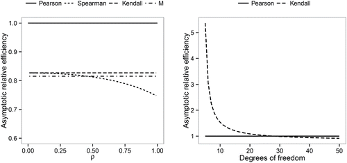
Figure 1 (left) displays the asymptotic efficiencies for different choices of R at the multivariate normal distribution with varying maximum correlation ρ. The rank correlation measures and the M-association estimator yield good asymptotic efficiencies of about 80%. The asymptotic efficiencies of the Kendall correlation and the M-estimator are constant, with the former being slightly higher than the latter. For the Spearman correlation, the asymptotic efficiency decreases with increasing ρ. While it is similarly high as for the Kendall correlation initially, it eventually drops below the asymptotic efficiency of the M-estimator.

Figure 1. Asymptotic efficiencies of the weighting vector ${\alpha }_R$ for different choices of the projection index R: at the multivariate normal distribution, as function of the true maximum correlation ρ (left); at the multivariate t-distribution, as function of the degrees of freedom of this distribution (right).

The good efficiency properties of the Kendall correlation carry over to heavy tailed distributions. Using Equations (20(20) $$\begin{array}{c}\hfill \text{ASV}{({\alpha }_R,H_0)}_{jj}=\frac{1}{{\rho }_R^2{\kappa }_R^{\text{'}}{\left({\rho }_R\right)}^2}E\left[X_j^2{\text{IF}}_1^2\left((X_1,Y),R,F_{\rho }\right)\right]\end{array}$$(20) ) and (24(24) $$\begin{array}{c}\hfill \text{ARE}({\alpha }_R,H_0)=\frac{\text{ASV}{({\alpha }_{R_P},H_0)}_{jj}}{\text{ASV}{({\alpha }_R,H_0)}_{jj}}.\end{array}$$(24) ), we derived asymptotic relative efficiencies at the multivariate t-distribution of the weighting vectors based on the Kendall correlation. Calculation of the ASV is still possible in this case, using the fact that the function κ_K is the same for any elliptically symmetric distribution (see Hult and Lindskog 2002). It turns out that the relative efficiencies, as in the normal case, are neither depending on the dimension p nor on the value ρ. Figure 1 (right) plots the asymptotic relative efficiencies as a function of the degrees of freedom of the multivariate t-distribution. We see that the Kendall correlation outperforms the Pearson correlation for smaller degrees of freedom, while the latter only becomes more efficient for degrees of freedom larger than 27.

5. Alternate Grid Algorithm

Let ${\mathbf{x}}_1,\dots ,{\mathbf{x}}_n\in {\mathbb{R}}^p$ and ${\mathbf{y}}_1,\dots ,{\mathbf{y}}_n\in {\mathbb{R}}^q$ be the observed data with p ⩾ q. To simplify notation, let $\widehat{R}(\mathbf{a},\mathbf{b}):=\widehat{R}(({\mathbf{a}}^t{\mathbf{x}}_1,{\mathbf{b}}^t{\mathbf{y}}_1),\dots ,({\mathbf{a}}^t{\mathbf{x}}_n,{\mathbf{b}}^t{\mathbf{y}}_n))$ denote the sample version of the association measure R with projection directions $\mathbf{a}$ and $\mathbf{b}$. The aim is to maximize the projection index (25) $$\begin{array}{c}\hfill f(\mathbf{a},\mathbf{b})=|\widehat{R}(\mathbf{a},\mathbf{b})|.\end{array}$$(25)

If p = 2 and $\mathbf{b}$ is fixed, the problem of finding the maximum association reduces to maximizing the function $\theta \to f({(cos(\theta ),sin(\theta \left)\right)}^t,\mathbf{b})$ over the interval [ − π/2, π/2). This can easily be solved with a grid search, that is, by dividing the interval in (N_g − 1) equal parts and evaluating the function at the grid points ( − 1/2 + j/N_g)π for j = 0, …, N_g − 1. The advantages of the grid search are that differentiability of the function is not required and that a global maximum can be distinguished from a local one. With a large enough number of grid points N_g, the found maximum will be close enough to the real solution.

If p > 2 and $\mathbf{b}$ being kept fixed, a sequence of optimizations in two-dimensional subspaces of the $\mathbf{X}$ space is performed. Given a weighting vector $\mathbf{a}$, its kth component a_k can be updated by a grid search in the subspace spanned by $\mathbf{a}$ and ${\mathbf{e}}_k^p$, the kth canonical basis vector of ${\mathbb{R}}^p$. For a grid of values for the angle θ as described above, the candidate directions are then given by (26) $$\begin{array}{c}\hfill t_k^p(\mathbf{a},\theta )=\frac{cos\left(\theta \right)\mathbf{a}+sin\left(\theta \right){\mathbf{e}}_k^p}{\sqrt{1+sin\left(2\theta \right)a_k}},\end{array}$$(26) where the denominator ensures unit norm of the candidate directions. This is done for k = 1, …, p. $R(\widehat{\mathit{}\mathbf{\alpha }},\widehat{\mathit{}\mathbf{\beta }})<0\mathrm{then\; set}\widehat{\mathit{}\mathbf{\beta }}\leftarrow -\widehat{\mathit{}\mathbf{\beta }}$

Hence, the idea of the algorithm is to perform series of grid searches, alternating between searching for $\mathbf{a}$ with a given $\mathbf{b}$ (as described above) and searching for $\mathbf{b}$ with a given $\mathbf{a}$. For details, see Algorithm 1. In the first cycle, the whole plane is scanned in each grid search. In the subsequent cycles, the search is limited to a more and more narrow interval of angles while keeping the number of grid points N_g constant. Moreover, the alternate series of grid searches in each cycle is stopped if the improvement is smaller than a certain threshold. Typically only very few iterations are necessary in each cycle, thus keeping computation time low.

If p > 1 and q = 1, the algorithm reduces to the algorithm of Croux, Filzmoser, and Oliveira (2007) with projection index (27) $$\begin{array}{c}\hfill f_y\left(\mathbf{a}\right):=\left|\widehat{R}(({\mathbf{a}}^t{\mathbf{x}}_1,y_1),\dots ,({\mathbf{a}}^t{\mathbf{x}}_n,y_n))\right|.\end{array}$$(27) The algorithm can be extended to higher-order (robust) canonical correlations by transforming the data into suitable subspaces along the lines of Branco et al. (2005). Our implementation for the statistical computing environment R is available in package ccaPP, which can be downloaded from http://CRAN.R-project.org/package=ccaPP.

6. Example

We present an application for the maximum rank correlation estimators in the regression setting. We use the movies data, which are available from http://had.co.nz/data/movies/ and contain movie information from the internet movie database (IMDb; http://imdb.com). The response variable is given by the average IMDb user rating, and we use the following p = 11 predictors: year of release, total budget in U.S. dollars, length in minutes, number of IMDb users who gave a rating, as well as a set of binary variables representing if the movie belongs to the genre action, animation, comedy, drama, documentary, romance, or short film. We limit the analysis to movies with known budget, leaving n = 5215 observations in the dataset.

We compare the four estimators based on maximum association measures with least-square (LS) regression and the robust MM-regression estimator tuned for 85% efficiency (e.g., Maronna, Martin, and Yohai 2006). Theoretically, LS regression gives the same results as the maximum Pearson correlation and is included to verify our numeric algorithm. We estimate the prediction performance by randomly splitting the data into training and test sets. We repeat this process L = 1000 times and use m = ⌊n/3⌋ observations as test data in each replication. As prediction loss, we use Spearman’s footrule distance (28) $$\begin{array}{c}\hfill d=\frac{1}{m}\sum _{i=1}^m|r_i-{\widehat{r}}_i|,\end{array}$$(28) where $\mathbf{r}={(r_1,\dots ,r_m)}^t$ are the ranks of the movies according to the average user rating and $\widehat{\mathbf{r}}={({\widehat{r}}_1,\dots ,{\widehat{r}}_m)}^t$ the predicted ranks.

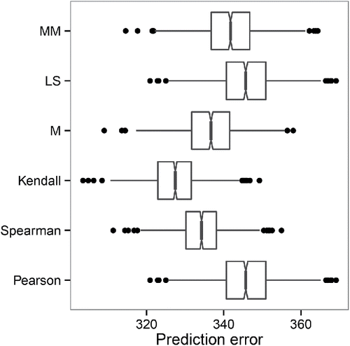
Figure 2 contains boxplots of the distribution of the prediction error for the considered methods. The maximum rank correlation estimators perform better than their competitors, with the Kendall correlation yielding the lowest prediction error. This hints at a nonlinear relationship between the response and the predictors, which we confirmed by inspecting plots of the response against the fitted values (not shown). The M-association estimator still results in quite good prediction performance, followed by the MM-regression estimator, the Pearson correlation, and LS. The latter two thereby give practically identical results, being in line with the theory. All prediction methods that we compare are linear in the predictor variables. Nonlinear methods as random forests might give even better prediction results.

Figure 2. Distribution of the prediction loss for the ranking according to the average IMDB user rating in the movies data, estimated via 1000 random splits into training and test data.

7. Simulation Experiments

The results presented here are a representative selection from an extensive simulation study. We focus on the case of p > 1 and q = 1. The sample counterparts of the maximum association measures and the weighting vectors are denoted by ${\widehat{\rho }}_R$ and ${\widehat{\alpha }}_R$. We compare the mean squared error (MSE) of the estimators ${\kappa }_R^{-1}\left({\widehat{\rho }}_R\right)$ and ${\widehat{\alpha }}_R$ of ρ and $\alpha$, respectively, for different projection indices R.

Additional experiments with different data configurations, sample sizes and dimensions are discussed in a supplementary report (Alfons, Croux, and Filzmoser 2016). In particular, we investigate the case of q > 1, yielding similar conclusions on the behavior of the estimators. The other additional experiments include an empirical bias study and a comparison of the power of permutation tests for detecting nonlinear relationships.

In each of the L = 1000 simulation runs, observations (x₁, y₁), …, (x_n, y_n) with ${\mathbf{x}}_i\in {\mathbb{R}}^p$ and $y_i\in \mathbb{R}$ are generated from the model distribution $N(\mathbf{0},\Sigma )$. We take (29) $$\begin{array}{c}\hfill \Sigma =\left(\begin{array}{cc}\hfill \mathbf{I}& \hfill {\Sigma }_{XY}\\ \hfill {\Sigma }_{YX}& \hfill 1\end{array}\right)\end{array}$$(29) with ${\Sigma }_{XY}={{\Sigma }_{YX}}^t={(\rho ,0,\dots ,0)}^t$. Thus, the true weighting vector is given by $\alpha ={(1,0,\dots ,0)}^t$, yielding the true maximum correlation ρ. We selected the sample size as n = 100 and the dimension of the x_i as p = 5.

For the estimators of the maximum correlation ρ, the mean squared error (MSE) is computed as (30) $$\begin{array}{c}\hfill {\text{MSE}}_R\left(\rho \right)=\frac{1}{L}\sum _{l=1}^L{\left(\varphi \left({\kappa }_R^{-1}\left({\widehat{\rho }}_R^l\right)\right)-\varphi \left(\rho \right)\right)}^2,\end{array}$$(30) where φ(ρ) = tanh ^{− 1}(ρ) is the Fisher transformation of ρ, which is often applied to render the finite sample distribution of correlation coefficients more toward normality, and ${\widehat{\rho }}_R^l$ is the estimated maximum association from the lth simulation run. For the weighting vectors, the MSE is computed as (31) $$\begin{array}{c}\hfill {\text{MSE}}_R\left(\alpha \right)=\frac{1}{L}\sum _{l=1}^L{\left\{{cos}^{-1}\left(\frac{|{\alpha }^t{\widehat{\alpha }}_R^l|}{\left|\right|\alpha \left|\right|\left|\right|{\widehat{\alpha }}_R^l\left|\right|}\right)\right\}}^2,\end{array}$$(31) where ${\widehat{\alpha }}_R^l$ is the estimated weighting vector from the lth simulation run. The measure (31(31) $$\begin{array}{c}\hfill {\text{MSE}}_R\left(\alpha \right)=\frac{1}{L}\sum _{l=1}^L{\left\{{cos}^{-1}\left(\frac{|{\alpha }^t{\widehat{\alpha }}_R^l|}{\left|\right|\alpha \left|\right|\left|\right|{\widehat{\alpha }}_R^l\left|\right|}\right)\right\}}^2,\end{array}$$(31) ) is the average of the squared angles between the vectors ${\widehat{\alpha }}_R^l$ and $\alpha$, making the MSE invariant to the choice of the normalization constraint for the weighting vectors.

For q = 1, an alternative procedure is the rank transformation least-square estimator of Garnham and Prendergast (2013). There the response variable Y is replaced by the corresponding ranks, and the weighting vector is then obtained by least-square regression of those ranks on the variables in $\mathbf{X}$. In the supplementary report (Alfons, Croux, and Filzmoser 2016), we add this estimator to the simulation study and show that this approach suffers from leverage points, that is, outliers in the space of the $\mathbf{X}$-variables. In absence of leverage points, it performs well.

7.1 Effect of a Nonlinear Monotonic Transformation

The true regression model is (32) $$\begin{array}{c}\hfill y_i={\mathbf{a}}^t{\mathbf{x}}_i+e_i,\end{array}$$(32) where the regression coefficients $\mathbf{a}$ are related to the weighting vector $\alpha$ through rescaling, that is, $\alpha =\mathbf{a}/\parallel \mathbf{a}\parallel$. We transform the response variable to ${\tilde{y}}_i=exp\left(y_i\right)$. Then we compute the different estimators once for the data (x_i, y_i) that follow the model and once for the data $({\mathbf{x}}_i,{\tilde{y}}_i)$ that do not follow the model. We thereby compare the results for varying maximum correlation ρ ∈ [0, 1).

Figure 3(a) and 3(b) shows the MSEs of the maximum association measures for the correctly specified model and the misspecified model, respectively. For the correctly specified model, the methods behave as expected: the Pearson correlation performs best, followed by the M-association estimator and the Spearman and Kendall correlation. However, the results are very different for the misspecified model. As long as the true maximum correlation ρ is small to moderate, the nonlinearity of the relationship is masked by the noise and all methods yield similar results. But as ρ increases, the MSEs of the Pearson correlation and (to a lesser extent) the M-association estimator drift away from 0. The rank correlation measures, on the other hand, are unaffected by the monotonic transformation.

Figure 3. MSEs of the maximum association measures (top) and the weighting vectors (bottom) for the correctly specified model (left) and for the misspecified model (right). In (b) and (d), the lines for the Spearman and Kendall correlation almost coincide. In (c), the lines for all methods except the Pearson correlation almost coincide.

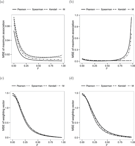
In Figure 3(c) and 3(d), the MSEs of the weighting vectors are displayed for the correctly^{Figure 4}specified model and the misspecified model, respectively. The nonlinear transformation does not have a very large effect on the MSE of the estimators. Still, while the Pearson correlation yields the best performance under the correctly specified model, the rank correlation measures perform better in the case of the misspecified model. Since the weighting vectors can be seen as normalized regression coefficients, we also computed two regression estimators: least squares (LS) and the robust MM-regression estimator tuned for 85% efficiency (e.g., Maronna, Martin, and Yohai 2006). We did not include those estimators in the plots to keep them from being overloaded. As expected from theory, LS gave the same results as the Pearson correlation, which underlines that our numerical algorithm works very well. In addition, the MM-estimator resulted in a slightly larger MSE than the Pearson correlation, yielding the largest MSE among all methods for the misspecified model.

7.2. Effect of Contamination

In the second simulation experiment, we investigate the effect of contamination on the estimators. We fix the true maximum correlation at ρ = 0.5. A fraction ϵ of the data is then replaced by outliers (x*_i, y*_i) coming from an $N({\mu }^{*},{\Sigma }^{*})$ distribution, where ${\mu }^{*}={(0,-5,0,0,0,5)}^t$ and ${\Sigma }^{*}$ is obtained from $\Sigma$ in (29(29) $$\begin{array}{c}\hfill \Sigma =\left(\begin{array}{cc}\hfill \mathbf{I}& \hfill {\Sigma }_{XY}\\ \hfill {\Sigma }_{YX}& \hfill 1\end{array}\right)\end{array}$$(29) ) by replacing ${\Sigma }_{XY}={{\Sigma }_{YX}}^t$ with ${\Sigma }_{XY}^{*}={{\Sigma }_{YX}^{*}}^t={(0,-1,0,0,0)}^t$. We vary the contamination level ϵ from 0% to 20% in steps of 2%.

Figure 4(a) shows the resulting MSEs of the maximum association measures. Clearly, the outliers have a strong influence on the Pearson correlation. For the M-estimator, the MSE remains low for small contamination levels but increases dramatically afterward. The rank correlation measures, on the other hand, are much less influenced by the outliers.

Figure 4. MSEs of the maximum association measures (left) and the weighting vectors (right) for varying percentage of contamination ϵ.

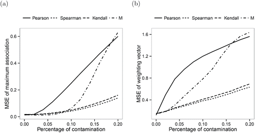
The MSEs for the corresponding weighting vectors are depicted in Figure 4(b). Again, the Pearson correlation is strongly influenced by the outliers. Concerning the M-association estimator, the outliers have a more immediate effect on the weighting vector than they have on the maximum association. As before, the maximum rank correlation estimators are more robust against the outliers. Furthermore, the results for the Spearman and Kendall correlation are very similar, confirming the theoretical results for the asymptotic variances.

8. Conclusions

This article studies a measure of association between two multivariate random vectors based on projection pursuit. Its definition is intuitively appealing: it is the highest possible association R between any two projections ${\alpha }^t\mathbf{X}$ and ${\beta }^t\mathbf{Y}$ constructed from the variables $\mathbf{X}$ and $\mathbf{Y}$. Using different projection indices R, different measures of association are obtained. For studying the robustness of the maximum association measures, we carry out influence calculations, showing that the projection index R should have a bounded and smooth influence function. In addition, we emphasize the important special case of univariate Y, in which case the problem of finding the projection yielding maximum association can be interpreted as a regression problem. Using maximum rank correlation estimators then has the advantage that they are invariant against monotonic transformations of the response. To study the robustness of the maximum association estimators against model misspecification and contamination, we present a simulation study and real data applications. Both the theoretical and the numerical results favor maximum rank correlation estimators, as they combine good robustness properties with good efficiency.

The derived influence functions and asymptotic variances can be used to obtain estimates of the standard errors of the coefficients of the weighting vectors. We obtain tractable expressions of the influence functions and asymptotic variances assuming an elliptically symmetric distribution. When the normality assumption does not hold, we suggest to use a bootstrap procedure. Note that Sherman (1993) developed standard errors for the Kendall-based weighting vector in the regression case q = 1, using numerical derivation.

We present an approximative algorithm to compute the proposed estimators via projection pursuit. Note that the rank correlation measures are fast to compute. Computation time of the Spearman correlation is dominated by computing the ranks of the two variables, which requires O(nlog n) time. While the definition of the Kendall rank correlation would suggest a computation time of O(n²), Knight (1966) introduced an O(nlog n) algorithm. The fast algorithm for the Kendall rank correlation is implemented in the R package ccaPP, together with the maximum association estimators.

Finally, as a topic for future research, other robustness measures such as breakdown point or maximum asymptotic bias could be derived as a complement to the influence function, which only considers infinitesimal contamination values.

Supplementary Materials

A supplementary report contains further technical details, a proof of Theorem 1, as well as an extensive collection of numerical results.

Acknowledgment

Parts of this research were done while Andreas Alfons was a Postdoctoral Research Fellow, Faculty of Economics and Business, KU Leuven, Leuven, Belgium. The authors thank the associate editor and three anonymous referees for their constructive remarks that substantially improved their article.

References

- Alfons, A., Croux, C., and Filzmoser, P. (2016), “Robust Maximum Association Estimators: Technical Supplement,” Supplementary Report.
- Branco, J. A., Croux, C., Filzmoser, P., and Oliveira, M. R. (2005), “Robust Canonical Correlations: A Comparative Study,” Computational Statistics, 20, 203–229.
- Breiman, L., and Friedman, J. (1985), “Estimating Optimal Transformations for Multiple Regression and Correlation,” Journal of the American Statistical Association, 80, 580–619.
- Croux, C., and Dehon, C. (2010), “Influence Functions of the Spearman and Kendall Correlation Measures,” Statistical Methods & Applications, 19, 497–515.
- Croux, C., Filzmoser, P., and Oliveira, M. (2007), “Algorithms for Projection-Pursuit Robust Principal Component Analysis,” Chemometrics and Intelligent Laboratory Systems, 87, 218–225.
- Garnham, A. L., and Prendergast, L. A. (2013), “A Note on Least Squares Sensitivity in Single-index Model Estimation and the Benefits of Response Transformations,” Electronic Journal of Statistics, 7, 1983–2004.
- Hampel, F. R., Ronchetti, E. M., Rousseeuw, P. J., and Stahel, W. (1986), Robust Statistics: The Approach Based on Influence Functions, New York: Wiley.
- Han, A. K. (1987), “Non-Parametric Analysis of a Generalized Regression Model: The Maximum Rank Correlation Estimator,” Journal of Econometrics, 35, 303–316.
- Huber, P. J. (1981), Robust Statistics, New York: Wiley.
- Hult, H., and Lindskog, F. (2002), “Multivariate Extremes, Aggregation and Dependence in Elliptical Distributions,” Advances in Applied Probability, 34, 587–608.
- Jin, J., and Cui, H. J. (2010), “Asymptotic Distributions in the Projection Pursuit Based Canonical Correlation Analysis,” Science China–Mathematics, 53, 485–498.
- Johnson, R. A., and Wichern, D. W. (2002), Applied Multivariate Statistical Analysis ( 5th ed.), Upper Saddle River, NJ: Prentice Hall.
- Knight, W. R. (1966), “A Computer Method for Calculating Kendall’s Tau With Ungrouped Data,” Journal of the American Statistical Association, 61, 436–439.
- Kudraszow, N. L., and Maronna, R. A. (2011), “Robust Canonical Correlation Analysis: A Predictive Approach,” available at http://www.mate.unlp.edu.ar/publicaciones/06062011164242.pdf
- López Blázquez, F., and Salamanca Miño, B. (2014), “Maximal Correlation in a Non-Diagonal Case,” Journal of Multivariate Analysis, 131, 265–278.
- Maronna, R., Martin, D., and Yohai, V. (2006), Robust Statistics: Theory and Methods, Chichester, UK: Wiley.
- Maronna, R. A. (1976), “Robust M-estimators of Multivariate Location and Scatter,” The Annals of Statistics, 4, 51–67.
- Papadatos, N., and Xifara, T. (2013), “A Simple Method for Obtaining the Maximal Correlation Coefficient and Related Characterizations,” Journal of Multivariate Analysis, 118, 102–114.
- Ramsay, J. O., Ten Berge, J., and Styan, G. P. H. (1984), “Matrix Correlation,” Psychometrika, 49, 403–423.
- Sherman, R. P. (1993), “The Limiting Distribution of the Maximum Rank Correlation Estimator,” Econometrica, 61, 123–137.
- Smilde, A. K., Kiers, H. A. L., Bijlsma, S., Rubingh, C. M., and van Erk, M. J. (2009), “Matrix Correlations for High-Dimensional Data: The Modified RV-Coefficient,” Bioinformatics, 25, 401–405.
- Taskinen, S., Croux, C., Kankainen, A., Ollila, E., and Oja, H. (2006), “Influence Functions and Efficiencies of the Canonical Correlation and Vector Estimates Based on Scatter and Shape Matrices,” Journal of Multivariate Analysis, 97, 359–384.
- Yu, Y. (2008), “On the Maximal Correlation Coefficient,” Statistics and Probability Letters, 78, 1072–1075.