Changepoint Detection in the Presence of Outliers

ABSTRACT

Many traditional methods for identifying changepoints can struggle in the presence of outliers, or when the noise is heavy-tailed. Often they will infer additional changepoints to fit the outliers. To overcome this problem, data often needs to be preprocessed to remove outliers, though this is difficult for applications where the data needs to be analyzed online. We present an approach to changepoint detection that is robust to the presence of outliers. The idea is to adapt existing penalized cost approaches for detecting changes so that they use loss functions that are less sensitive to outliers. We argue that loss functions that are bounded, such as the classical biweight loss, are particularly suitable—as we show that only bounded loss functions are robust to arbitrarily extreme outliers. We present an efficient dynamic programming algorithm that can find the optimal segmentation under our penalized cost criteria. Importantly, this algorithm can be used in settings where the data needs to be analyzed online. We show that we can consistently estimate the number of changepoints, and accurately estimate their locations, using the biweight loss function. We demonstrate the usefulness of our approach for applications such as analyzing well-log data, detecting copy number variation, and detecting tampering of wireless devices. Supplementary materials for this article are available online.

Keywords:

• Binary segmentation
• Biweight loss
• Cusum
• M-estimation
• Penalized likelihood
• Robust statistics

1. Introduction

Changepoint detection has been identified as one of the major challenges for modern, big data applications (National Research Council 2013). The problem arises when analyzing data that can be ordered, for example, time-series or genomics data where observations are ordered by time or position on a chromosome, respectively. Changepoint detection refers to locating points in time or position where some aspect of the data of interest, such as location, scale, or distribution, changes. There has been an explosion in methods for detecting changes (e.g., Frick, Munk, and Sieling 2014; Fryzlewicz 2014; Cao and Wu 2015; Ma and Yau 2016; Haynes, Fearnhead, and Eckley 2017b, and references therein) in recent years, in part motivated by the range of applications for which changepoint detection is important. Exemplar areas of application include bioinformatics (Olshen et al. 2004; Futschik et al. 2014), ion channels (Hotz et al. 2013), climate records (Reeves et al. 2007), oceonagraphic data (Killick et al. 2010; Killick, Fearnhead, and Eckley 2012), and finance (Kim, Morley, and Nelson 2005).

What has received less attention is the problem of distinguishing between changepoints and outliers. To give an example of the issue outliers can cause when attempting to detect changepoints, consider the problem of detecting changes in well-log data. An example of such data, taken originally from Ó Ruanaidh and Fitzgerald (1996), is shown in Figure 1. This data was collected from a probe being lowered into a bore-hole. As it is lowered, the probe takes measurements of the rock that it is passing through. As the probe moves from one type of rock strata to another, there is an abrupt change in the measurements. It is these changes in rock strata that we wish to detect. The real motivation for collecting this data was to detect these changes in real time. This would enable changes in rock strata that are being drilled through to be quickly detected, so that appropriate changes to the settings of the drill can be made.

Figure 1. Well-log data: data with outliers removed (left column) and original data (right column). Bottom row shows segmentations of the data under a least squares loss.

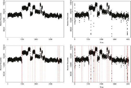
The data in the top-left plot in Figure 1 has been analyzed by many different change detection methods (e.g., Ó Ruanaidh and Fitzgerald 1996; Fearnhead 2006; Adams and MacKay 2007; Wyse et al. 2011; Ruggieri and Antonellis 2016). However, this plot actually shows data that has been preprocessed to remove outliers. The real data that was collected by the probe is shown in the top-right plot of Figure 1. There are a number of short periods of time where the probe misfunctions, and very low measurements are recorded. These are examples of what we are calling outliers. The real challenge with detecting the changes is to distinguish between actual changes and these outliers. Most existing methods for changepoint detection are unable to do so; hence, the reason that most analyses of this data has used the “cleaned” dataset in the top-left plot. For example, in the bottom row of Figure 1, we show the results of estimating the changepoints based on minimizing a square-error-loss criteria with a penalty for each detected changepoint. While this method performs well when analyzing the cleaned dataset, it is unable to distinguish between changes and outliers when analyzing the real data.

This lack of robustness for detecting a change in mean in the presence of outliers for many changepoint methods stems from explicit or implicit assumptions of Gaussian noise. For example, methods based on a likelihood-ratio test for detecting a change (Worsley 1979), or that use a penalized likelihood approach to detect multiple changes (Killick, Fearnhead, and Eckley 2012), or that do a Bayesian analysis (Yao 1984), may be based on a Gaussian likelihood and thus explicitly assume Gaussian noise. Alternative methods, such as using an L₂ (square error) loss or a cusum-based approach (Page 1954), may not make such an assumption explicitly. However, the resulting methods are closely related to those based on a Gaussian likelihood (see, e.g., Hinkley 1971), and thus are implicitly making similar assumptions. While these methods show some robustness to heavier tailed noise (Lavielle and Moulines 2000), in practice they can seriously over-estimate the number of changes in the presence of outliers.

Our approach is based on the ideas from robust statistics, namely replacing an L₂ loss with an alternative loss function that is less sensitive to outliers. We then use such a loss function within a penalized cost approach to estimating multiple changepoints. The use of alternative loss functions as a way to make changepoint detection robust to ouliers has been considered before (e.g., Hušková and Sen 1989; Hušková 1991; Hušková and Picek 2005; Hušková 2013). That work derives cusum-like tests for a single changepoint. Such a test for a single changepoint can then be used with binary segmentation to find multiple changes. As we discuss more fully in Section 2.3, this approach suffers from the drawback that the test statistic is based upon how well the data can be modeled as not having a change, and does not directly compare this with how well we can fit the data with one or more changepoints. Thus, it could spuriously infer a change if we have a cluster of outliers at consecutive time-points, even if the value of those outliers are not consistent with them coming from the same distribution.

One challenge with the penalized cost approach that we suggest is minimizing this cost, which we need to do to infer the changepoints. We show how recent efficient dynamic programming algorithms (Rigaill 2015; Maidstone et al. 2017) can be adapted to solve this minimization problem. Our algorithm can use any loss function provided we are interested in the change of univariate parameter, such as the location parameter for univariate data, and the loss function is piecewise quadratic. Importantly, these algorithms are sequential in nature, and thus can be directly applied in situations, which need an online analysis of the data.

While our approach can be used with a range of loss functions, we particularly recommend using a loss function that is bounded. We present a theoretical result which shows that we need a bounded loss function if we wish our method to be robust to any single outlier. The simplest such loss function is the biweight loss (Huber 2011), which is the pointwise minimum of an L₂ loss and a constant. We show that, under mild conditions, we can consistently estimate the number of changepoints, and accurately estimate their locations, if we use a penalized cost approach with the biweight loss.

To illustrate the usefulness of our approach with the biweight loss, we present its use for three distinct applications. The first is for the online analysis of the well-log data of Figure 1. Second, we show that it out-performs existing methods for detecting copy number (CN) variation. This includes performing better than methods that preprocess the data in an attempt to remove outliers. By comparison, our approach is easier to implement as it does not require any preprocessing steps. Finally, we consider the problem of detecting tampering of wireless security devices. Results here show our method can reliably distinguish between actual tampering events and changes in the data caused by short-term environmental factors.

Proofs of results are given in the Appendices in the supplementary material. Code implementing the new methods in this article is available from https://github.com/guillemr/robust-fpop.

2. Model Definition

Assume, we have data ordered by some covariate, such as time or position along a chromosome. Denote the data by $\mathbf{y}=(y_1,\cdots ,y_n)$. We will use the notation that, for s ⩽ t, the set of observations from time s to time t is y_{s: t} = (y_s, …, y_t). If we assume that there are k changepoints in the data, this will correspond to the data being split into k + 1 distinct segments. We let the location of the jth changepoint be τ_j for $j=1,\cdots ,k$, and set τ₀ = 0 and τ_{k + 1} = n. The jth segment will consist of data points $y_{{\tau }_{j-1}+1},\dots ,y_{{\tau }_j}$. We let τ = (τ₀, …, τ_{k + 1}) be the set of changepoints.

The statistical problem we are considering is how to infer both the number of changepoints and their locations. We assume the changepoints correspond to abrupt changes in the location, that is mean, median, or other quantile, of the data. We will focus on a minimum penalized cost approach to the problem. This approach encompasses penalized likelihood approaches to changepoint detection among others.

To define our penalized cost, we first introduce a loss function for a single observation, y, and a segment-specific location parameter θ. We denote this as γ(y; θ). For a penalized likelihood approach, this loss would be equal to minus the log-likelihood. The class of losses, we will consider are discussed below.

We can now define the cost associated with a segment of data, y_{s: t}. This is $$\mathcal{C}\left(y_{s:t}\right)=\underset{\theta }{min}\sum _{i=s}^t\gamma (y_i;\theta ),$$the minimum, over the segment-specific parameter θ, of the sum of the losses associated with each observation in the segment. The penalized cost for a segmentation is then (1) $$\begin{array}{c}\hfill Q(y_{1:n};{\tau }_{1:k})=\sum _{i=0}^k\left\{\mathcal{C}\left(y_{{\tau }_i+1:{\tau }_{i+1}}\right)+\beta \right\}\end{array}$$(1) where β > 0 is a chosen constant that penalizes the introduction of changepoints. We estimate the number and position of the changepoints by the value of k and τ_{1: k} that minimize this penalized cost. The value of β has a substantial impact on the number of changepoints that are estimated (see Haynes, Eckley, and Fearnhead 2017a, for examples of this), with larger values of β leading to fewer estimated changepoints.

For inferring changes in the mean of the data, it is common to use the square-error-loss function (e.g., Yao and Au 1989; Lavielle and Moulines 2000). $$\gamma (y;\theta )={(y-\theta )}^2.$$In this case, the penalized cost approach corresponds to a penalized likelihood approach, where the data within a segment are iid Gaussian with common variance. Minimizing a penalized cost of this form is closely related to binary segmentation procedures based on cusum statistics (e.g., Vostrikova 1981; Bai 1997; Fryzlewicz 2014), as discussed in Killick, Fearnhead, and Eckley (2012). Use of the square-error-loss function results in an approach that is very sensitive to outliers. For example, this loss function was the one used in the analysis of the well-log data in Figure 1, where we saw that it struggles to distinguish outliers from actual changes of interest.

2.1. Penalized Costs Based on M-Estimation

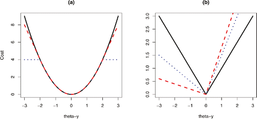
To develop a changepoint approach that can reliably detect changepoints in the presence of outliers we need a loss function that increases at a slower rate in |y − θ|. Standard examples (Huber 2011) are absolute error, γ(y; θ) = |y − θ|, Huber loss $$\gamma (y;\theta )=\left\{\begin{array}{cc}\hfill {(y-\theta )}^2& \hfill \text{if}|y-\theta |<K,\\ \hfill 2K|y-\theta |-K^2& \hfill \text{otherwise,}\end{array}\right.$$and the biweight loss (2) $$\begin{array}{c}\hfill \gamma (y;\theta )=\left\{\begin{array}{cc}\hfill {(y-\theta )}^2& \hfill \text{if}|y-\theta |<K,\\ \hfill K^2& \hfill \text{otherwise,}\end{array}\right.\end{array}$$(2) or if interest lies in changes in the uth quantile for 0 < u < 1 $$\gamma (y;\theta )=\left\{\begin{array}{cc}\hfill 2u(y-\theta )& \hfill \text{if}y>\theta ,\\ \hfill 2(1-u)(\theta -y)& \hfill \text{otherwise.}\end{array}\right.$$These are summarized in Figure 2.

Figure 2. Example of different losses. (a) The square error loss (full-line), and the related Huber loss (red dashed) and biweight loss (blue dotted). (b) The absolute error loss (full-line), and its generalization for detecting change in quantiles for u = 0.1 (red dashed) and u = 0.25 (blue dotted).

We will develop an algorithm for finding the best segmentation under a penalized cost criteria that can deal with any of these choices for the loss. In practice, we particularly advocate the use of the biweight loss. For a penalized cost approach to detecting changepoints to be robust to extreme outliers we will need the loss function to be bounded. For unbounded loss functions, such as the absolute error loss or Huber loss, a penalized cost approach will place an outlier in a segment on its own if that outlier is sufficiently extreme. This is shown by the following result.

Theorem 1.

Assume that the loss function satisfies γ(y; θ) = g(|y − θ|), where g(0) = 0 and g( · ) is an unbounded, increasing function. Choose any t ∈ {1, …, n} and fix the set of other observations, y_s for s ≠ t. Then, there exists values of y_t such that the segmentation that minimizes the penalized cost (1(1) $$\begin{array}{c}\hfill Q(y_{1:n};{\tau }_{1:k})=\sum _{i=0}^k\left\{\mathcal{C}\left(y_{{\tau }_i+1:{\tau }_{i+1}}\right)+\beta \right\}\end{array}$$(1) ) will have changepoints at t − 1 and t.

If we choose a loss function, such as the biweight loss, that is bounded, then this will impose a minimum segment length on the segmentations that we infer using the penalized cost function. Providing this minimum segment length is greater than 1, our inference procedure will be robust to the presence of extreme outliers—unless these outliers cluster at similar values, and for a number of consecutive time-points greater than our minimum segment length.

Theorem 2.

If the loss function satisfies 0 ⩽ γ(y; θ) ⩽ K, and we infer changepoints by minimizing the penalized cost function (1(1) $$\begin{array}{c}\hfill Q(y_{1:n};{\tau }_{1:k})=\sum _{i=0}^k\left\{\mathcal{C}\left(y_{{\tau }_i+1:{\tau }_{i+1}}\right)+\beta \right\}\end{array}$$(1) ) with penalty β for adding a changepoint, then all inferred segments will be of length greater than β/K.

The other conclusion to draw from this result is that, for any choice of K and β, we would want the minimum segment length to be smaller than any segment we expect, or that we wish to detect, in the data. Any real segments shorter than the minimum segment length are unlikely to be detected, with the observations in such short segments being identified as outliers instead. Furthermore, our procedure can lose power to detect real segments that are only slightly longer than the minimum segment length (see empirical results for scenario 4 in Section 5.2).

2.2. Consistency Under Biweight Loss

As mentioned above, and as suggested by Theorem 1, a particular focus will be on the use of the biweight loss (2(2) $$\begin{array}{c}\hfill \gamma (y;\theta )=\left\{\begin{array}{cc}\hfill {(y-\theta )}^2& \hfill \text{if}|y-\theta |<K,\\ \hfill K^2& \hfill \text{otherwise,}\end{array}\right.\end{array}$$(2) ). Here, we give conditions under which we can consistently estimate the number and location of changepoints when using this loss.

We will consider the standard in-fill asymptotics, as we let the number of data points, n, increase. To be able to consistently estimate the number of changepoints, we will need the penalty for adding a changepoint, β in (1(1) $$\begin{array}{c}\hfill Q(y_{1:n};{\tau }_{1:k})=\sum _{i=0}^k\left\{\mathcal{C}\left(y_{{\tau }_i+1:{\tau }_{i+1}}\right)+\beta \right\}\end{array}$$(1) ), to increase with n. We will thus denote the choice of penalty for a given number of data points to be β_n.

Data-Generating Model: We assume a fixed number of changepoints, k₀, and fixed constants $0<u_1<\cdots <u_{k_0}<1$ so that for a dataset of size n, we have the ith changepoint at τ_i = ⌊nu_i⌋, for i = 1, …, k₀. As above, we let τ₀ = 0 and ${\tau }_{k_0+1}=n$. We further assume fixed segment-specific location parameters, ${\mu }_0,\dots ,{\mu }_{k_0}$, with the obvious constraint that μ_i ≠ μ_{i − 1} for i = 1, …, k₀. Finally, we let Z₁, Z₂, … be iid noise random variables, so that for t = 1, …, n the observations are realizations of $$Y_t={\mu }_i+Z_t$$where i is such that τ_i < t ⩽ τ_{i + 1}.

Our results require two mild conditions on the distribution of the noise random variables. First, introduce the mean of the loss function, M(θ) = E{γ(Z_i; θ)}. We assume M(θ) takes it minimum value at θ = 0. We can make this assumption without loss of generality, as if M(θ) has its minimum at θ* we can just reparameterize our model with new noise random variables set to Z_i − θ* and with location parameters redefined to be μ_i + θ*.

Condition 1: Our first condition is that there exists constants c₁ > 0 and c₂ > 0 such that (3) $$\begin{array}{c}\hfill M\left(\theta \right)=\text{E}\left[min\left\{{(Z_i-\theta )}^2,K^2\right\}\right]\ge M\left(0\right)+min\left\{c_1{\theta }^2,c_2\right\}.\end{array}$$(3) This is a weak assumption, and will hold if M(θ) has a positive second derivative for all θ in a neighborhood around 0 and that M(θ) − M(0) ⩾ c₂ > 0 for all θ outside this region. The latter requirement is a common assumption made to ensure identifiability of estimates of a location parameter when using a given loss function.

Condition 2: Our second condition is slightly stronger. Let $p=Pr\left(\right|Z_i|>K)$ and σ² = E(Z²_i∣|Z_i| ⩽ K), then we need (4) $$\begin{array}{c}\hfill K^2(1-2p)-(1-p){\sigma }^2>0.\end{array}$$(4) This condition can be achieved by taking K large enough. If the noise has finite variance then, using Chebyshev’s inequality, it is easy to show that any choice with $K>\sqrt{3}\text{E}\left(Z_i^2\right)$ will ensure this condition holds. However, we do not need the noise to have a variance. For example, it is sufficient to choose $K>\sqrt{3}\text{E}(min\{Z_i^2,K^2\})$, or, if Z_i has a unimodal density function with mode at 0, then σ² ⩽ K²/3 and it suffices to choose K so that $p=Pr\left(\right|Z_i|>K)<2/5$. By comparison, we would recommend taking K sufficiently large that |Z_i| > K is relatively rare, and thus p ≈ 0. In line with Theorem 1, this condition does not depend on the distribution of the noise conditional on |Z_i| > K.

Theorem 3.

Consider the data generating model described above, and suppose conditions 1 and 2 hold. For a given n, let ${\widehat{k}}_n$ be the estimate of the number of changepoints, and ${\widehat{\tau }}_1,\dots ,{\widehat{\tau }}_{{\widehat{k}}_n}$ their estimated locations, obtained by minimizing the penalized cost (1(1) $$\begin{array}{c}\hfill Q(y_{1:n};{\tau }_{1:k})=\sum _{i=0}^k\left\{\mathcal{C}\left(y_{{\tau }_i+1:{\tau }_{i+1}}\right)+\beta \right\}\end{array}$$(1) ) using the biweight loss function and a penalty β_n. Then, there exists constants C₁ > 0 and C₂ > 0 such that $$\begin{array}{ccc}& & Pr\left[{\widehat{k}}_n=k_0\text{and}\underset{i=1,\dots ,k_0}{max}\left\{\underset{j=1,\dots ,{\widehat{k}}_n}{min}\left|{\tau }_i-{\widehat{\tau }}_j\right|\right\}\le C_{2}log\left(n\right)\right]\hfill \\ & & \to 1,\text{as}n\to \infty \text{,}\hfill \end{array}$$provided that C₁log (n) < β_n = o(n).

The theorem shows that for an appropriate choice of β_n, we can obtain a consistent estimate of the true number of parameters, and that the error in estimating any of the changepoint locations will be less than C₂log (n) with probability tending to 1. The latter order of error is in line with asymptotic results for the accuracy of changepoint estimates using wild binary segmentation with the cusum test Fryzlewicz (2014). We require much weaker conditions on the distribution of the noise, but our result assumes stronger conditions on the number of changes, the segment lengths and the size of change of mean at each changepoint than, for example, results in Fryzlewicz (2014) and Baranowski, Chen, and Fryzlewicz (2016). The result supports the use of a penalty, β_n, that is proportional to log (n), a choice that is common for other penalized cost procedures, but it does not specify the constant of proportionality.

2.3. Alternative Robust Changepoint Methods

There have been other proposed M-procedures for robust detection of changepoints (Hušková and Sen 1989; Hušková 1991; Hušková and Picek 2005; Hušková 2013). These differ from our approach in that they are based on sequentially applying tests for single changepoints. One approach is to use a Wald-type test. For a convex loss function, γ(y; θ), which depends only on y − θ, define γ(y; θ) = ρ(y − θ) and define φ to be the first derivative of ρ. Then, we can estimate a common θ for data y_{1: n} by minimizing $$\sum _{i=1}^n\rho (y_i-\theta ),$$with respect to θ. In many cases, this is equivalent to solving $$\sum _{i=1}^n\varphi (y_i-\theta )=0.$$If $\widehat{\theta }$ denotes the estimate we obtain, we can define residuals as $\varphi (y_i-\widehat{\theta })$, and their partial sums, or cusums, by $$S_m=\sum _{i=1}^m\varphi (y_i-\widehat{\theta }).$$A Wald-type test is then based on a test-statistic of the form $$T_n=\underset{1\le m\le n-1}{max}\frac{n}{m(n-m)}{S}_m^2,$$where the term n/(m(n − m)) is introduced so that the variability of the term on the right-hand side will be similar for each value of m. Large values of T_n are taken as evidence for a change. The position of a changepoint is then inferred at the position m that maximizes the right-hand side. To detect multiple changepoints, this Wald-type test needs is currently used within a binary segmentation procedure; though it can also be used with improved versions of binary segmentation, such as wild binary segmentation (Fryzlewicz 2014).

There are two main differences between the Wald-type test approach and our penalized cost approach. The first is that the Wald-type test statistic is appropriate only for convex loss functions. So, for example, the biweight loss is not appropriate for use with this approach. To see this note that the derivative of the biweight loss satisfies φ(x) = 0 for |x| > K. Thus, large abrupt changes in the data will lead to M-residuals which are 0, and hence provide no evidence for a change in the test statistic.

Second, any loss function that increases linearly in |y − θ| for sufficiently large |y − θ| will result in φ(y_i − θ) being constant for large |y_i − θ|. Thus, large residuals will have a bounded contribution to the test statistic. To see this, consider the Wald-type test with the Huber loss. To calculate this test statistic, we first calculate our estimate of the location parameter for the data, $\widehat{\theta }$, assuming the data is from a single segment. The ith residual is then K if $y_i>\widehat{\theta }+K$, − K if $y_i<\widehat{\theta }-K$, and $y_i-\widehat{\theta }$ otherwise. The cusum statistic is just the sum of these residuals. This is equivalent to winsorizing the data, where we shrink extreme positive or negative values to be K above or below our estimate of the location parameter, and then using a cusum test for detecting a changepoint. The actual value of the data points that are above $\widehat{\theta }+K$ or below $\widehat{\theta }-K$ will not affect the cusum values, and hence not affect the value of the Wald-type test statistic.

The use of Huber loss within a Wald-type test will thus have a similar robustness to extreme outliers that bounded loss functions have for the penalized cost approach. The main difference is that the Wald-type test statistic does not consider whether the data after a putative changepoint is consistent with data from a single segment. Thus, a cluster of outliers of the same sign that occur concurrently but which are very different in value, such as we observe for the well-log data, will produce a similar value for the test-statistic as a set of concurrent observations that are very different to the other data points but are also very similar to one another. By comparison, the penalized cost based approach would, correctly, say the latter provided substantially more evidence for the presence of a change.

3. Minimizing the Penalized Cost

An issue with detecting changepoints using any of these loss functions, is how can we efficiently minimize the resulting penalized cost over all segmentations? We present an efficient dynamic programming algorithm for performing this minimization exactly. This algorithm is an extension of the pruned dynamic programming algorithm of Rigaill (2015) and the FPOP algorithm of Maidstone et al. (2017) (see also Johnson 2013) to the robust loss functions. We will call the resulting algorithm R-FPOP.

3.1. A Dynamic Programming Recursion

We develop a recursion for finding the minimum cost (1(1) $$\begin{array}{c}\hfill Q(y_{1:n};{\tau }_{1:k})=\sum _{i=0}^k\left\{\mathcal{C}\left(y_{{\tau }_i+1:{\tau }_{i+1}}\right)+\beta \right\}\end{array}$$(1) ) of segmenting data y_{1: t} for t = 1, …, n. In the following, we let τ denote a vector of changepoints. Furthermore, we let ${\mathcal{S}}_t$ denote the set of possible changepoints for the y_{1: t}, so $${\mathcal{S}}_t=\left\{\mathit{}\mathbf{\tau }={\tau }_{1:k}:0<{\tau }_1<\cdots <{\tau }_k<t\right\}.$$Note that ${\mathcal{S}}_t$ has 2^{t − 1} elements. Define $$Q_t=\underset{\mathit{}\mathbf{\tau }\in {\mathcal{S}}_t}{min}Q(y_{1:t};{\tau }_{1:k})=\underset{\mathit{}\mathbf{\tau }\in {\mathcal{S}}_t}{min}\sum _{i=0}^k\left\{\mathcal{C}\left(y_{{\tau }_i+1:{\tau }_{i+1}}\right)+\beta \right\},$$where here and later we use the convention that k is the number of changepoints in τ, and that τ₀ = 0 and τ_{k + 1} = t. First, we introduce the minimum penalized cost of segmenting y_{1: t} conditional on the most recent segment having parameter θ, $$Q_t\left(\theta \right)=\underset{\mathit{}\mathbf{\tau }\in {\mathcal{S}}_t}{min}\left[\sum _{i=0}^{k-1}\left\{\mathcal{C}\left(y_{{\tau }_i+1:{\tau }_{i+1}}\right)+\beta \right\}+\sum _{j={\tau }_k+1}^t\gamma (y_j;\theta )+\beta \right],$$where we take the first summation on the right-hand side to be 0 if k = 0. Trivially, we have Q_t = min _θQ_t(θ) and Q₁(θ) = γ(y₁; θ) + β.

The idea is to recursively calculate Q_t(θ) for increasing values of t. To do this, we note that each element in ${\mathcal{S}}_t$ is either an element in ${\mathcal{S}}_{t-1}$ or an element in ${\mathcal{S}}_{t-1}$ with the addition of a changepoint at t − 1. So (5) $$\begin{array}{ccc}\hfill Q_t\left(\theta \right)& =& \underset{\mathit{}\mathbf{\tau }\in {\mathcal{S}}_{t-1}}{min}\left[min\left\{\sum _{i=0}^{k-1}\left(\mathcal{C}\left(y_{{\tau }_i+1:{\tau }_{i+1}}\right)+\beta \right)+\sum _{j={\tau }_k+1}^t\gamma (y_j;\theta )+\beta ,\right.\right.\hfill \\ & & \left.\left.\sum _{i=0}^k\left(\mathcal{C}\left(y_{{\tau }_i+1:{\tau }_{i+1}}\right)+\beta \right)+\gamma (y_t;\theta )+\beta \right\}\right]\hfill \\ & =& min\left\{\underset{\mathit{}\mathbf{\tau }\in {\mathcal{S}}_{t-1}}{min}\left[\sum _{i=0}^{k-1}\left(\mathcal{C}\left(y_{{\tau }_i+1:{\tau }_{i+1}}\right)+\beta \right)+\sum _{j={\tau }_k+1}^{t-1}\gamma (y_j;\theta )+\beta \right],\right.\hfill \\ & & \left.\underset{\mathit{}\mathbf{\tau }\in {\mathcal{S}}_{t-1}}{min}\left[\sum _{i=0}^k\left(\mathcal{C}\left(y_{{\tau }_i+1:{\tau }_{i+1}}\right)+\beta \right)+\beta \right]\right\}+\gamma (y_t;\theta )\hfill \\ & =& min\left\{Q_{t-1}\left(\theta \right),Q_{t-1}+\beta \right\}+\gamma (y_t;\theta ).\hfill \end{array}$$(5) The first equality comes from splitting the minimization into the minimization over the changepoints for y_{1: t − 1} and then whether there is or is not a changepoint at t − 1. The second equality comes from interchanging the order of the minimizations, and taking out the common γ(y_t; θ) term. The final equality comes from the definitions of Q_{t − 1}(θ) and Q_{t − 1}. The right-hand side just depends on Q_{t − 1}(θ), as Q_{t − 1} = min _θQ_{t − 1}(θ).

3.2. Solving the Recursion

We now show how we can efficiently solve the dynamic programming recursion from the previous section for loss functions like those introduced in Section 2. We make the assumption that the loss for any observation, γ(y_t; θ), viewed as function of θ, can be written as a piecewise quadratic in θ. Note that by quadratic, we include the special cases of linear or constant functions of θ, and this definition covers all the loss functions introduced in Section 2.

As the set of piecewise quadratics is closed under the both addition and minimzation, it follows that C_t(θ) can be written as a piecewise quadratic for all t. We summarize C_t(θ) by N_t intervals (a^(t)_i, b^(t)_i], and associated quadratics q^(t)_i(θ). We assume that the intervals are ordered, so a^(t)₁ = −∞, a^(t)_i = b^(t)_{i − 1} for i = 2, …, N_t and $b_{N_t}^{\left(t\right)}=\infty$. To make this summary of C_t(θ) unique, we further assume that q^(t)_i(θ) ≠ q_{i − 1}^(t)(θ) for i = 2, …, N_t. If this were not the case, we could merge the neighboring intervals.

We can split Equation (5(5) $$\begin{array}{ccc}\hfill Q_t\left(\theta \right)& =& \underset{\mathit{}\mathbf{\tau }\in {\mathcal{S}}_{t-1}}{min}\left[min\left\{\sum _{i=0}^{k-1}\left(\mathcal{C}\left(y_{{\tau }_i+1:{\tau }_{i+1}}\right)+\beta \right)+\sum _{j={\tau }_k+1}^t\gamma (y_j;\theta )+\beta ,\right.\right.\hfill \\ & & \left.\left.\sum _{i=0}^k\left(\mathcal{C}\left(y_{{\tau }_i+1:{\tau }_{i+1}}\right)+\beta \right)+\gamma (y_t;\theta )+\beta \right\}\right]\hfill \\ & =& min\left\{\underset{\mathit{}\mathbf{\tau }\in {\mathcal{S}}_{t-1}}{min}\left[\sum _{i=0}^{k-1}\left(\mathcal{C}\left(y_{{\tau }_i+1:{\tau }_{i+1}}\right)+\beta \right)+\sum _{j={\tau }_k+1}^{t-1}\gamma (y_j;\theta )+\beta \right],\right.\hfill \\ & & \left.\underset{\mathit{}\mathbf{\tau }\in {\mathcal{S}}_{t-1}}{min}\left[\sum _{i=0}^k\left(\mathcal{C}\left(y_{{\tau }_i+1:{\tau }_{i+1}}\right)+\beta \right)+\beta \right]\right\}+\gamma (y_t;\theta )\hfill \\ & =& min\left\{Q_{t-1}\left(\theta \right),Q_{t-1}+\beta \right\}+\gamma (y_t;\theta ).\hfill \end{array}$$(5) ) into two steps. The first is (6) $$\begin{array}{c}\hfill Q_t^{*}\left(\theta \right)=min\left\{Q_{t-1}\left(\theta \right),Q_{t-1}+\beta \right\},\end{array}$$(6) and the second is $$Q_t\left(\theta \right)=Q_t^{*}\left(\theta \right)+\gamma (y_t;\theta ).$$

For the first step, we calculate Q_{t − 1} by minimizing the N_{t − 1} quadratics defining Q_{t − 1}(θ) on their respective intervals, and then calculating the minimum of these minima. We then solve the minimization problem (6(6) $$\begin{array}{c}\hfill Q_t^{*}\left(\theta \right)=min\left\{Q_{t-1}\left(\theta \right),Q_{t-1}+\beta \right\},\end{array}$$(6) ) on each of the N_{t − 1} intervals. For interval i, the solution will either be q^(t)_i(θ), Q_{t − 1} + β, or we will need to split the interval into two or three smaller intervals, on which the solution will change between q^(t)_i(θ) and Q_{t − 1} + β. Thus, we will end with a set of N_{t − 1}, or more, ordered intervals and corresponding quadratics that define Q*_t(θ). We then prune these intervals by checking whether any neighboring intervals both take the value Q_{t − 1} + β, and merging these if they do. This will lead to a new set of N*_t, say, ordered intervals, and associated quadratics, q*_{t, i}(θ) say.

For each of the N*_t intervals from the output of the minimization problem, we then add γ(y_t; θ) to the corresponding q*_{t, i}(θ). This may involve splitting the ith interval into two or more smaller intervals if one or more of the points of change of the function γ(y_t; θ) are contained in it. This will lead to the N_t intervals and corresponding quadratics that define Q_t(θ).

The above describes how we recursively calculate Q_t(θ). In practice, we also want to then extract the optimal segmentation under our criteria. This is straightforward to do. For each of the intervals corresponding to different pieces of Q_t(θ), we can associate a value of the most recent changepoint prior to t. When we evaluate Q_t, we need to find which interval contains this value, and then the optimal value for the most recent changepoint prior to t is the value associated with that interval. We can store these optimal values for all t, and after processing all data we can recursively track back through these values to extract the optimal segmentation. So, we would first find the value of the most recent changepoint prior to n, τ say, then find the value of the most recent changepoint prior to τ. We repeat this until the most recent changepoint is at 0, corresponding to no earlier changepoints.

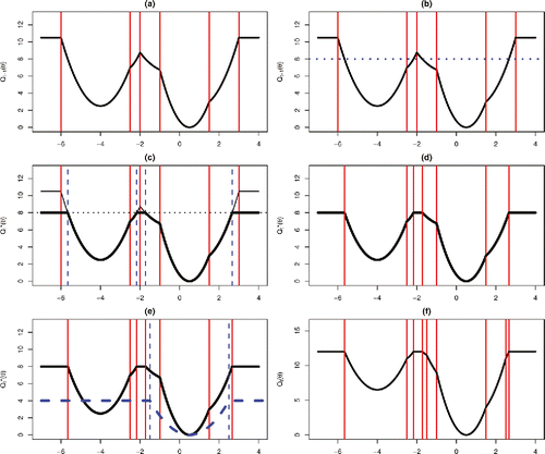
Pseudo-code for R-FPOP is given in Appendix D. An example of the steps involved in one iteration is given in Figure 3.

Figure 3. Example of one iteration of R-FPOP: (a) Q_{t − 1}(θ) (black solid line), and set of intervals stored (split by vertical red lines) at start of iteration. (b) Find the pointwise minimum of Q_{t − 1}(θ) and Q_{t − 1} + β (blue dashed line). (c) This is done by solving the minimization on each interval, which splits some intervals into two or three. New splits are shown by blue dashed vertical lines. (d) Merge neighboring intervals if they both take the value Q_{t − 1} + β. (e) Now add the loss for the new observation (blue dashed curve). (f) This further splits intervals at the points where the form of γ(y_t; θ) changes, the blue vertical lines in plot (e). Shown is the final representation of Q_t(θ). At all stages only piecewise quadratic functions need to be stored.

4. Computational Cost of R-FPOP

We now present results that bound the computational cost and storage requirements of R-FPOP. As above, we will assume that γ(y; θ) can be written as a piecewise quadratic with L pieces. The bounds that we get differ depending on whether γ(y; θ) is convex in θ. We first consider the convex case, which includes all the examples in Section 2 except the biweight loss.

Theorem 4.

If γ is convex in θ and defined in L pieces R-FPOP stores at most 2t − 1 + t(L − 1) quadratics and intervals at step t.

Corollary 1.

If γ is convex in θ and defined in L pieces, the space complexity of R-FPOP is $\mathcal{O}\left(n\right)$, and the time complexity of R-FPOP is $\mathcal{O}\left(n^2\right)$.

For the biweight loss, which is not convex, we get worse bounds on the complexity of R-FPOP.

Theorem 5.

For the biweight loss R-FPOP stores $\mathcal{O}\left(t^2\right)$ intervals at step t.

Corollary 2.

For the biweight loss R-FPOP has worst-case space complexity that is $\mathcal{O}\left(n^2\right)$, and time complexity that is $\mathcal{O}\left(n^3\right)$.

These results give worst-case bounds on the time and storage complexity of R-FPOP. Below, we investigate empirically the time and storage cost and observe an average computational cost that is linear in n when the number of changepoints is large and less than quadratic when there is no changepoint.

5. Results

5.1. Simulation Study: Computational Cost

This article is mostly concerned with the statistical performances of our robust estimators. Thus, an in-depth analysis of the runtime of our approach is outside the scope of this article. In this section, we just aim at showing that our approach is easily applicable to large profiles (n = 10³ to n = 10⁶) in the sense that its runtime is comparable to other commonly used approach like FPOP (Maidstone et al. 2017), PELT (Killick, Fearnhead, and Eckley 2012), Wild Binary Segmentation (WBS) (Fryzlewicz 2014), or smuceR (Frick, Munk, and Sieling 2014).

We used a standard laptop with an Intel Core i7-3687U CPU with 2.10 GHz × 4 Core and 7.7 Gb of RAM. For the biweight loss, for a profile of length n = 10⁶ and in the absence of any true change the runtime is around 4 sec (slightly larger than FPOP, see Figure 4, left L₂). As a matter of comparison on the same computer the runtime of competitor methods WBS, PELT, and smuceR for a profile of length n = 10⁵ are, respectively, around 7 sec, 40 sec, and 175 sec. For an increasing number of changes runtimes are smaller (see Figure 4, right). Runtimes for the L₁ and Huber loss are quite a bit larger: in the absence of changes and for n = 10⁶ the L₁ runtime is around 500 sec and the Huber runtime is around 200 sec (see Figure 4, left).

Figure 4. Runtime in seconds of R-FPOP for different loss functions. We simulated profiles with n going from 2000 to 1,024,000, with or without changes and using iid Gaussian noise. The axes use a log-scale, and we have added lines of slope 1 (dashed) and 2 (dotted).

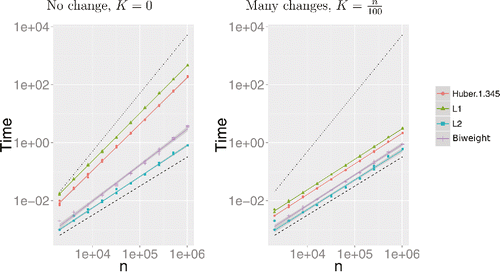
Most importantly, we see that with many changepoints, the average CPU cost of all penalized cost approaches increases only linearly with the number of data points (parallel to the dashed black line in Figure 4, right). With no changepoints, the average CPU cost increases faster in particular for the L₁ and Huber losses, however, it is less than quadratic (slopes smaller than the dotted black line in Figure 4, left). The CPU cost of the biweight loss is very close to the CPU cost of the L₂ loss.

5.2. Simulation Study: Accuracy

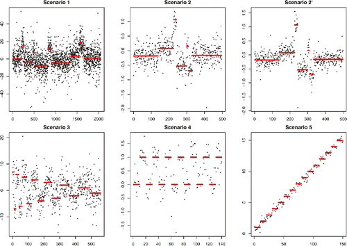
We assessed the performance of our robust estimators using the simulation benchmark proposed in the WBS article (Fryzlewicz 2014). In that article, five scenarios are considered. These vary in length from n = 150 to n = 2048 and contain a variety of short and long segments, and a variety of sizes of the change in location from one segment to the next. We considered an additional scenario from Frick, Munk, and Sieling (2014) corresponding to scenario 2 of WBS with a standard deviation of 0.2 rather than 0.3. In our simulation study, we are interested to see how the presence of outliers or heavy-tailed noise affect different changepoint methods, and so we will test each method assuming t-distributed noise. The underlying signals and example data for the three scenarios are shown in Figure 5.

Figure 5. The signal, and example data, for each of the scenarios considered for the simulation study. Data were generated with the noise having a t-distribution with five degrees of freedom.

For all approaches, we need to choose the value K in the loss function and the penalty/threshold for adding a changepoint. These will depend on the standard deviation of the noise. Our approach is to estimate this standard deviation using the median absolute deviation of the differenced time-series, as in Fryzlewicz (2014), which we denote as $\widehat{\sigma }$. We compared our various robust estimators (Huber and biweight loss) to binary segmentation using the robust cusum test (Hušková and Sen 1989), described in Section 2.3 (Cusum). For the biweight loss, we chose $K=3\widehat{\sigma }$, so that extreme residuals according to a Gaussian model are treated as outliers. For the Huber loss, we chose $K=1.345\widehat{\sigma }$, a standard choice for trading statistical efficiency of estimation with robustness. We further set the penalty/threshold to be $\beta =2{\widehat{\sigma }}^{2}log\left(n\right)\text{E}\left(\varphi {\left(Z\right)}^2\right)$, where φ is the gradient of the loss function and Z is a standard Gaussian random variable. This is based on the Schwarz information criteria, adapted to account for the variability of loss function that is used (see, e.g., theoretical results in Hušková and Marušiaková 2012, for further justification of this), and for the biweight loss this is inline with Theorem 3, which suggested the use of a penalty that is proportional to log (n). We also compared to just using the standard square-error loss: implemented using FPOP (Maidstone et al. 2017); and to the WBS (Fryzlewicz 2014) approach that uses a standard cusum test statistic for detecting changepoints. Again, we used $\beta =2{\widehat{\sigma }}^{2}log\left(n\right)\text{E}\left(\varphi {\left(Z\right)}^2\right)$, which in this case simplifies to the standard Bayesian Information Criteria (BIC) penalty $\beta =2{\widehat{\sigma }}^{2}log\left(n\right)$, and is the value that gave the best results for these methods across the six scenarios when there is normal noise (see Maidstone et al. 2017).

We consider analyzing data where the noise was from a t-distribution. We vary the degrees of freedom from 3 to 100 to see of how varying how heavy-tailed the noise is affects the performance of different methods.

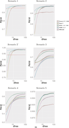
In Figures 6 and 7, we show the results of all approaches as a function of the degrees of freedom. We compare methods based on how they well estimate the underlying piecewise constant mean function, measured in terms of mean square error; and how well they estimate the segmentation, measured using the normalized rand-index. The normalized rand-index measures the overlap between the true segmentation and the inferred segmentation, with larger values indicating a better estimation of the segmentation.

Figure 6. Smoothed log mean square error (MSE) of all tested approaches on the six scenarios using a student-noise with the degrees of freedom ranging from 3 to 100.

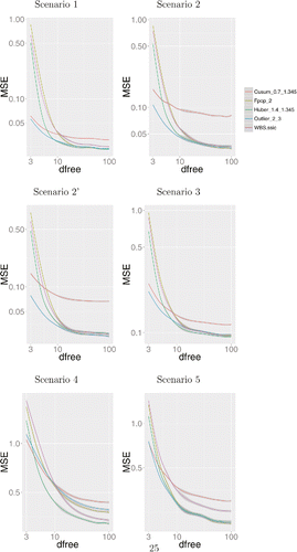
Figure 7. Smoothed normalized Rand-index of all tested approaches on the six scenarios using student-noise with the degrees of freedom varying from 3 to 100.

In terms of mean square error, for almost all scenarios, we consider the biweight loss performs the best when the degrees of freedom are small. It also appears to lose little in terms of accuracy when the degrees of freedom is large, and the noise is close to Gaussian. The robust cusum approach also performs well when the degrees of freedom are small, but in most cases it shows a marked drop in accuracy relative to the alternative methods when the noise is close to Gaussian. The one scenario where the biweight loss performs poorly when the noise is close to Gaussian is Scenario 4. In this case, we have short segments, only slightly larger than the minimum segment length for the biweight loss, with the segment mean being the same for all odd segments. We can get a reasonable fit under the biweight loss by, for example, ignoring the changepoints and treating all observations in the even segments as outliers. The problem of distinguishing between this case and the presence of actual changepoints causes the poor performance.

The results in terms of the quality of the segmentation, as measured using the rand-index, are more mixed. The biweight loss is clearly best in scenarios 1 and 2, but performs poorly for scenario 3. Here, the use of the Huber loss appears to give the best results across the different scenarios. Again, we see that the use of the L2 loss, using either FPOP or WBS, performs poorly when the degrees of freedom are small.

5.3. Online Analysis of Well-Log Data

We return to the well-log data of Figure 1. For this data, due to the presence of substantial outliers, we choose to use the biweight loss function. We set the threshold, K in (2(2) $$\begin{array}{c}\hfill \gamma (y;\theta )=\left\{\begin{array}{cc}\hfill {(y-\theta )}^2& \hfill \text{if}|y-\theta |<K,\\ \hfill K^2& \hfill \text{otherwise,}\end{array}\right.\end{array}$$(2) ), to be twice an estimate of the standard deviation of the observation noise. We set β to be 70 times the estimated variance of the noise. This is larger than that of the BIC penalty, but this is needed due to the presence of autocorrelation in the observation noise (Lavielle and Moulines 2000), and is the same penalty used for the analysis presented in Figure 1.

Figure 8 shows the estimated changepoints, we obtain from a batch analysis of the data. As we can see, using the biweight penalty makes the changepoint detection robust to the presence of the outliers. All obvious changes are detected, and we do not detect a change at any point where the outliers cluster.

Figure 8. Estimated changepoints from batch analysis of the well-log data (left-hand plot) under biweight loss. Estimate of location of most-recent changepoint from online analysis (right-hand plot). The black line shows the estimate of the most-recent changepoint against the number of data points analyzed. The red dashed horizontal lines show the locations of the changepoints detected from the batch analysis.

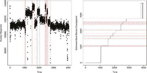
As mentioned in the introduction, the motivation for analyzing this data requires an online analysis. We present output from such an online analysis in the right-hand plot of Figure 8. Here, we plot the estimate of the most recent changepoint prior to t, given data y_{1: t}, as a function of t. To help interpret the result, we also show the locations of the changepoints inferred from the batch analysis. We see that we are able to quickly detect changes when they happen, and we have only one region where there is some fluctuation in where we estimate the most recent changepoint. While by eye the plot may suggest we immediately detect the changes, there is actually some lag. This is inevitable when using the biweight loss, due to the presence of a minimum segment length that can be inferred (see Theorem 2). The lag in detecting the changepoint is between 21 and 27 observations for all except the final changepoint. The final inferred changepoint is less pronounced, and is not detected until after a lag of 40 observations. This lag can be reduced by increasing K, but at the expense of less robustness to outliers. The region of fluctuation over the estimate of the most recent changepoint corresponds to uncertainty about whether there are changepoints in the last inferred segment (corresponding to the final two changepoints inferred in the bottom-left plot of Figure 1). One disadvantage of detection methods that involve minimizing a penalized cost, and of other methods that produce a single estimate of the changepoint locations, is that they do not quantify the uncertainty in the estimate.

5.4. Estimating Copy Number Variation

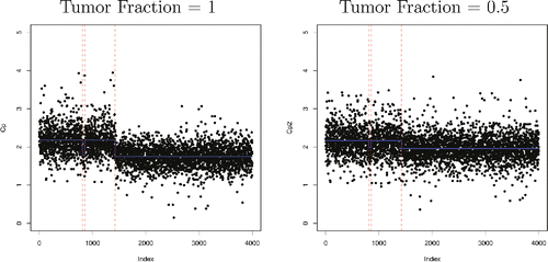
Healthy human cells have two copies of DNA. In tumor cells, parts of chromosomes of various sizes (from kilobases to a chromosome arm) may be deleted or amplified several times, and this can lead to the copy number (CN) of the DNA from such regions being different from 2. CN can be measured using microarray or sequencing experiments. They are piecewise constant along the genome, and interest lies in detecting whether, and where, the CN changes. For many samples, we would have a mixture of healthy and tumor cells, and the signal-to-noise ratio for changes in CN will go down with the tumor fraction. The detection of changes in CN is further complicated by the presence of outliers. We illustrate this in Figure 9 using output from the jointseg package (Pierre-Jean, Rigaill, and Neuvial 2015) that enables simulation of realistic CN profiles by resampling real datasets for which the truth is known.

Figure 9. Two DNA copy number profiles obtained using the jointseg package with a tumor fraction of 1 (left) and 0.5 (right). The true changepoints are represented with red dotted lines. It can be seen that a number of data-points are quite far from the blue line. The size of each jump is larger when the tumor fraction is larger.

A standard way to analyze such data is to use the smooth. CNA function of the well-known DNAcopy package (Bengtsson et al. 2016). This function shrinks outliers toward the value of its neighbors. Once this is done one can run a preferred segmentation approach. As we will see below, this heuristic preprocessing procedure greatly improves changepoint detection. We want to compare such a two-stage approach to a simpler analysis, where we analyze data using our penalized cost approach with the biweight loss.

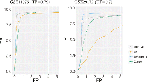
To assess the performance of our approach on DNA CN data, we used the jointseg package. We simulated profiles of length n = 4000 with 10 change-points with segments of at least 40 data-points. The package propose two real datasets, GSE11976 and GSE29172, to resample from. For both, we considered four levels of difficulty corresponding to different tumor fractions: 0.34, 0.50, 0.79, and 1 for GSE11976; and 0.3, 0.5, 0.7, and 1 for GSE29172.

We consider four approaches: FPOP (L2), FPOP after using smooth. CNA to remove outliers (Rout L2), robust binary segmentation (Cusum), and our biweight loss with a threshold value of 3. All approaches are implemented for a range of penalty values. For every simulated profile and each run of a method, we computed the number of true positive (TP) and false positive (FP) change-points. For all true change-point, we counted one TP if there is at least one change-point identified within a window of 15 data-points. We then computed the number of FPs as the number of predicted changes minus the number of TPs. We then average, over 200 simulated profiles, the number of TPs and FPs per approach, penalty value and difficulty to recover receiver operating characteristic (ROC) curves.

Overall our robust biweight loss outperforms the L2 loss following outlier removal and the Cusum approach. For low tumor fractions (0.3 and 0.5 GSE29172 and 0.34 GSE11976), the biweight loss is possibly slightly better than the Cusum approach. For a tumor fraction of 1, the biweight loss is slightly better than the L2 following outlier removal. In other cases, it is clearly better. Results are shown for the two datasets and a tumor fraction of 0.7 and 0.79 in Figure 10. Results for other tumor fractions are provided in figures in Appendix E.

Figure 10. Average ROC curve on the GSE11976 and GSE29172 datasets for a tumor fraction of, respectively, 0.79 and 0.7, for the Cusum, L2, L2 with outlier removal (Rout L2) and our robust biweight loss (Biweight 3).

5.5. Wireless Tampering

We now consider an application that looks at security of the Internet of Things (IoT). Many IoT devices use WiFi to communicate. Often, for example, with surveillance systems, these need a high level of security. Thus, it is important to be able to detect if a device has been tampered with. WiFi signals include a “preamble,” which is used by the receiver to determine channel state. One approach that can be used to detect tampering is to monitor channel state variation (Bagci 2016). Abrupt changes in it could indicate some tampering event. However, changes can also be caused by less sinister events, such as movement of people within the communication environment. Thus, the challenge is to detect a change caused by tampering as opposed to any “outliers” caused by such temporary environmental factors.

Figure 11 shows some time-series of channel state information (CSI) that has been extracted from the preamable from a signal sent by a single IoT device. This data is taken from Bagci et al. (2015), where a controlled experiment was performed, with an actual tampering event occurring after 22 min. Before this tampering event, there was movement of people around the device, which has a short-term effect on the time-series data.

Figure 11. Examples from the analysis of the wireless tampering data. We show six examples of the data, with different structure before and after a change, and with different patterns of outliers caused by temporary environmental factors. In each case, there is a single changepoint, after 22 min (denoted by the triangle). The inferred changepoint (vertical dashed line) and inferred mean function (green full horizonal line) from our method with the biweight loss function are shown in each case.

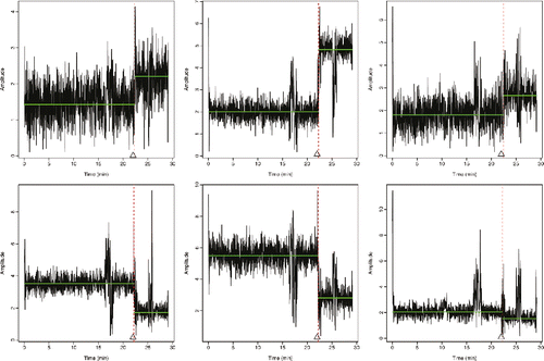
In practice, the CSI from an IoT device is multi-dimensional, and we show time-series for 6 out of 90 dimensions. While ideally, we would jointly analyze the data from all 90 time-series that we get from the device, we will just consider analyzing each time-series individually. Our interest is to see how viable it is to use our approach, with the biweight loss, to accurately distinguish between tampering event and any effects due to temporary environmental factors. The six time-series we show each show different patterns, both in terms of the change caused by tampering, and the effect of people walking near the device. As such they give a thorough testing of any approach. We implemented the biweight loss with the Schwarz Information Criteria penalty for a change, and with K chosen so that the minimum segment length (see Theorem 2) corresponds to a period of 20 sec. Results are shown in Figure 11, where we see that we accurately only detect the change that corresponds to the tampering event in all cases.

6. Discussion

We have presented an algorithm for detecting changepoints by minimizing a penalized cost, which measures fit to the data by a loss function that is piecewise quadratic. In particular, we have shown that by using bounded loss functions we can develop algorithms that are robust to the presence of arbitrarily large outliers. We particular recommend the use of the biweight loss function, and have shown that using such a loss function can lead to the consistent estimation of the number of changepoints and accurate estimation of their location under weak conditions on the noise distribution.

If we use the biweight loss, we have to choose an appropriate value for K. To some extent this is a modeling decision, but a reasonable default is to choose this to be around 2–3 times an estimate of the standard deviation of the noise. This will mean the loss performs similarly to the square-error loss, as most observations will be within K of the segment location parameter, but with the added benefit of robustness to extreme outliers.

We have shown that using the biweight loss with a penalty for adding a changepoint that is C₁log (n) for some suitable constant C₁ can lead to consistent estimation of the number of changepoints. If K is chosen as suggested, it is natural to choose C₁ to be similar to choices that are known to work well with the square-error loss, as we did within Section 5.2. Such choices are not guaranteed to produce large enough constants to ensure consistency. If this is a concern, it is possible to use the idea behind that strengthened Schwarz information criteria of Fryzlewicz (2014), and choose a penalty C₁(log n)^{1 + ε} for some small ε > 0.

Care must be taken if there are violations of the iid assumption for the noise. In such cases, it is known that consistent estimation of the number of changepoints is still possible if we appropriately inflate the penalty (Lavielle and Moulines 2000), and we would suggest using a similar inflation when using the biweight loss. Choosing how much to inflate is difficult in practice, and thus it makes sense to try a range of penalties (which can be done efficiently, e.g., using the CROPS algorithm of Haynes, Eckley, and Fearnhead 2017a). For applications that involve analyzing multiple similar datasets, we would recommend using a small set of training data to help choose an appropriate constant (see, e.g., Rigaill et al. 2013).

Finally, the joint choice of K and β can be informed by the minimum segment length that can be inferred for such a choice; see Theorem 2. To have robustness to extreme outliers we need this minimum segment length to be greater than 1. Equally, it should be chosen to be smaller than the shortest segment we wish to identify. This choice is linked to the question of how many similar observations would we require before we would classify them as coming from a new segment as opposed to being correlated outliers.

Supplementary Material

The supplementary material contains Appendices in which proofs of results are given.

Acknowledgments

The authors thank Utz Roedig and Ethem Bagci for supplying and discussions around the wireless tampering data, and to Lawrence Bardwell for help with analyzing this data.

Additional information

Funding

This work was supported by EPSRC grant EP/N031938/1 (StatScale) and an ATIGE grant from Génopole.

References

- Adams, R. P., and MacKay, D. J. (2007), “Bayesian Online Changepoint Detection,” arXiv: 0710.3742.
- Bagci, I. E. (2016), “Novel Security Mechanisms for Wireless Sensor Networks,” PhD dissertation, Lancaster University, Lancaster, UK.
- Bagci, I. E., Roedig, U., Martinovic, I., Schulz, M., and Hollick, M. (2015), “Using Channel State Information for Tamper Detection in the Internet of Things,” in Proceedings of the 31st Annual Computer Security Applications Conference, pp. 131–140.
- Bai, J. (1997), “Estimating Multiple Breaks One at a Time,” Econometric Theory, 13, 315–352.
- Baranowski, R., Chen, Y., and Fryzlewicz, P. (2016), “Narrowest-Over-Threshold Detection of Multiple Change-Points and Change-Point-Like Features,” arXiv:1609.00293.
- Bengtsson, H., Neuvial, P., Seshan, V. E., Olshen, A. B., Spellman, P. T., and Olshen, R. A. (2016), “Package pscbs,” available at ftp://ftp.parrot.org/.1/cran/web/packages/PSCBS/PSCBS.pdf
- Cao, H., and Wu, W. B. (2015), “Changepoint Estimation: Another Look at Multiple Testing Problems,” Biometrika, 102, 974–980.
- Fearnhead, P. (2006), “Exact and Efficient Inference for Multiple Changepoint Problems,” Statistics and Computing, 16, 203–213.
- Frick, K., Munk, A., and Sieling, H. (2014), “Multiscale Change-Point Inference,” Journal of the Royal Statistical Society, Series B, 76, 495–580.
- Fryzlewicz, P. (2014), “Wild Binary Segmentation for Multiple Change-Point Detection,” Annals of Statistics, 42, 2243–2281.
- Futschik, A., Hotz, T., Munk, A., and Sieling, H. (2014), “Multiscale DNA Partitioning: Statistical Evidence for Segments,” Bioinformatics, 30, 2255–2262.
- Haynes, K., Eckley, I. A., and Fearnhead, P. (2017a), “Computationally Efficient Changepoint Detection for a Range of Penalties,” Journal of Computational and Graphical Statistics, 26, 134–143.
- Haynes, K., Fearnhead, P., and Eckley, I. (2017b), “A Computationally Efficient Nonparametric Approach for Changepoint Detection,” Statistics and Computing, 27, 1293–1305.
- Hinkley, D. V. (1971), “Inference About the Change-Point From Cumulative Sum Tests,” Biometrika, 58, 509–523.
- Hotz, T., Schütte, O. M., Sieling, H., Polupanow, T., Diederichsen, U., Steinem, C., and Munk, A. (2013), “Idealizing Ion Channel Recordings by a Jump Segmentation Multiresolution Filter,” IEEE Transactions on Nanobioscience, 12, 376–386.
- Huber, P. J. (2011), “Robust Statistics,” in International Encyclopedia of Statistical Science, eds. M. Lovric. Berlin: Springer.
- Hušková, M. (1991), “Recursive M-Tests for the Change-Point Problem, in Economic Structural Change, eds. P. Hackl and A. H. Westlund. Berlin: Springer, pp. 13–33.
- ——— (2013). “Robust Change Point Analysis,” in Robustness and Complex Data Structures. Springer, pp. 171–190.
- Hušková, M., and Marušiaková, M. (2012), “M-Procedures for Detection of Changes for Dependent Observations,” in Communications in Statistics-Simulation and Computation, 41, 1032–1050.
- Hušková, M., and Picek, J. (2005), “Bootstrap in Detection of Changes in Linear Regression,” Sankhyā: The Indian Journal of Statistics, 67, 200–226.
- Hušková, M., and Sen, P. K. (1989), “Nonparametric Tests for Shift and Change in Regression at an Unknown Time Point,” in Statistical Analysis and Forecasting of Economic Structural Change. Springer, pp. 71–85.
- Johnson, N. A. (2013), “A Dynamic Programming Algorithm for the Fused Lasso and l0-Segmentation,” Journal of Computational and Graphical Statistics, 22, 246–260.
- Killick, R., Eckley, I. A., Ewans, K., and Jonathan, P. (2010), “Detection of Changes in Variance of Oceanographic Time-Series Using Changepoint Analysis,” Ocean Engineering, 37, 1120–1126.
- Killick, R., Fearnhead, P., and Eckley, I. A. (2012), “Optimal Detection of Changepoints With a Linear Computational Cost,” Journal of the American Statistical Association, 107, 1590–1598.
- Kim, C.-J., Morley, J. C., and Nelson, C. R. (2005), “The Structural Break in the Equity Premium,” Journal of Business & Economic Statistics, 23, 181–191.
- Lavielle, M., and Moulines, E. (2000), “Least-Squares Estimation of an Unknown Number of Shifts in a Time Series,” Journal of Time Series Analysis, 21, 33–59.
- Ma, T. F., and Yau, C. Y. (2016), “A Pairwise Likelihood-Based Approach for Changepoint Detection in Multivariate Time Series Models,” Biometrika, 103, 409–421.
- Maidstone, R., Hocking, T., Rigaill, G., and Fearnhead, P. (2017), “On Optimal Multiple Changepoint Algorithms for Large Data,” Statistics and Computing, 27, 519–533.
- National Research Council (2013), Frontiers in Massive Data Analysis, Washington, DC: The National Academies Press, https://doi.org/10.17226/18374.
- Olshen, A. B., Venkatraman, E. S., Lucito, R., and Wigler, M. (2004), “Circular Binary Segmentation for the Analysis of Array-Based DNA Copy Number Data,” Biostatistics, 5, 557–72.
- ÓRuanaidh, J. J. K., and Fitzgerald, W. J. (1996), Numerical Bayesion Methods Applied to Signal Processing, New York: Springer.
- Page, E. (1954), “Continuous Inspection Schemes,” Biometrika, 41, 100–115.
- Pierre-Jean, M., Rigaill, G., and Neuvial, P. (2015), “Performance Evaluation of DNA Copy Number Segmentation Methods,” Briefings in Bioinformatics, 16, 600–615.
- Reeves, J., Chen, J., Wang, X. L., Lund, R., and Lu, Q. Q. (2007), “A Review and Comparison of Changepoint Detection Techniques for Climate Data,” Journal of Applied Meteorology and Climatology, 46, 900–915.
- Rigaill, G. (2015), “A Pruned Dynamic Programming Algorithm to Recover the Best Segmentations With 1 to Kmax Change-Points,” Journal de la Société Française de Statistique, 156, 180–205.
- Rigaill, G., Hocking, T. D., Bach, F., and Vert, J.-P. (2013), “Learning Sparse Penalties for Change-Point Detection Using Max Margin Interval Regression,” in Proceedings of the 30th International Conference on Machine Learning, JMLR W&CP (vol. 28), pp. 172–180.
- Ruggieri, E., and Antonellis, M. (2016), “An Exact Approach to Bayesian Sequential Change Point Detection,” Computational Statistics & Data Analysis, 97, 71–86.
- Vostrikova, L. (1981), “Detection of the Disorder in Multidimensional Random-Processes,” Doklady Akademii Nauk SSSR, 259, 270–274.
- Worsley, K. (1979), “On the Likelihood Ratio Test for a Shift in Location of Normal Populations,” Journal of the American Statistical Association, 74, 365–367.
- Wyse, J., Friel, N., (2011), “Approximate Simulation-Free Bayesian Inference for Multiple Changepoint Models With Dependence Within Segments,” Bayesian Analysis, 6, 501–528.
- Yao, Y.-C. (1984), “Estimation of a Noisy Discrete-Time Step Function: Bayes and Empirical Bayes Approaches,” The Annals of Statistics, 12, 1434–1447.
- Yao, Y.-C., and Au, S. (1989), “Least-Squares Estimation of a Step Function,” Sankhyā: The Indian Journal of Statistics, Series A, 51, 370–381.