Nonparametric Estimation of Copula Regression Models With Discrete Outcomes

Abstract

Multivariate discrete outcomes are common in a wide range of areas including insurance, finance, and biology. When the interplay between outcomes is significant, quantifying dependencies among interrelated variables is of great importance. Due to their ability to accommodate dependence flexibly, copulas are being applied increasingly. Yet, the application of copulas on discrete data is still in its infancy; one of the biggest barriers is the nonuniqueness of copulas, calling into question model interpretations and predictions. In this article, we study copula estimation with discrete outcomes in a regression context. As the marginal distributions vary with covariates, inclusion of continuous regressors expands the region of support for consistent estimation of copulas. Because some properties of continuous outcomes do not carry over to discrete outcomes, specification of a copula model has been a problem. We propose a nonparametric estimator of copulas to identify the “hidden” dependence structure for discrete outcomes and develop its asymptotic properties. The proposed nonparametric estimator can also serve as a diagnostic tool for selecting a parametric form for copulas. In the simulation study, we explore the performance of the proposed estimator under different scenarios and provide guidance on when the choice of copulas is important. The performance of the estimator improves as discreteness diminishes. A practical bandwidth selector is also proposed. An empirical analysis examines a dataset from the Local Government Property Insurance Fund (LGPIF) in the state of Wisconsin. We apply the nonparametric estimator to model the dependence among claim frequencies from different types of insurance coverage. Supplementary materials for this article are available online.

Keywords:

• Copula specification
• Identifiability
• Insurance claim frequency

1 Introduction

Multivariate discrete outcomes are common in a wide scope of areas, including insurance, psychometrics, and epidemiology. For instance, in property insurance, it is common that a policy contains multiple coverage types, for example, building and contents (BC) coverage and motor vehicle (MV) coverage, so that the analyst may observe multiple outcomes, one from each coverage type. When the interplay between outcomes has significant consequences, modeling dependencies among interrelated variables is of great importance. In the foregoing example, quantifying dependencies among risks is critical for understanding the uncertainty of the portfolio, and thus is important for an insurer’s solvency and profitability.

There are many good approaches available for modeling multivariate discrete outcomes. Generalized linear mixed models (McCulloch and Neuhaus 2005) have been extensively applied to handle correlated discrete observations, though the models do not keep the marginal distributions after integrating out random effects. For binary data, models such as multinomial logistic regression, dependence ratios, and odds ratios approaches are widely used, cf., Frees, Jin, and Lin (2013). None of these models appears to be uniformly preferable to the others. The existing literature also contains a variety of models for multivariate counts. One commonly used approach of introducing dependencies among counts is through common additive errors, for instance, a multivariate Poisson model with a common covariance parameter (Johnson, Kotz, and Balakrishnan 1997). Multivariate negative binomial distributions (Winkelmann 2000) and zero-inflated multivariate Poisson models (Bermúdez and Karlis 2011) can be applied in the presence of overdispersion. A limitation of the foregoing models is that they allow only positive correlations. There are models that allow negative correlations, such as multivariate Poisson-log-normal models (Aitchison and Ho 1989) and the correlated latent effects approach (Chib and Winkelmann 2001). However, for some datasets, different marginal models than the commonly used ones or combinations of different marginal models might be necessary (Frees, Lee, and Yang 2016).

This paper uses a probabilistic structure known as a copula, which is a multivariate distribution function with uniform margins and has been used to study dependencies in many areas including, but not limited to, insurance (Frees and Valdez 1998), finance (Li 1999), and survival analysis (Shih and Louis 1995); see Nelsen (2006) for an introduction. Sklar’s theorem (Sklar 1959) provides a theoretical foundation for copulas as useful tools to connect margins and dependence that the joint distribution can be expressed in terms of margins and a copula. Sklar’s theorem is unified over continuous, discrete, and mixture cases. Parametric copulas can be fit through maximum likelihood estimation (MLE) straightforwardly, and there are numerous copula families which can accommodate different dependence structures such as negative correlations, asymmetry, and tail dependence (Joe 1993; Yang, Frees, and Zhang 2011).

Copulas are commonly applied in the regression settings in which outcomes are related to a set of covariates (Song, Li, and Yuan 2009). Copula regression can preserve the solid body of work established for marginal models (e.g., McCullagh and Nelder 1989) and accommodate dependence structures flexibly. Each marginal distribution can be specified to be conditioned on its covariates. It is customary to assume a dependence structure that is constant over observations. We use this simplifying assumption in this article for the purposes of identifiability and easy interpretation; see alternatives in Nikoloulopoulos and Karlis (2008).

Although most applications focus on continuous variables, there is an increasing trend in the application of copulas on discrete data. For binary outcomes, the widely used multivariate probit model (Brown 1998) is indeed a special case of copula regression models using probit margins and a Gaussian copula (Song 2007). For more applications, Nikoloulopoulos and Karlis (2008) and Genest et al. (2013) modeled multivariate binary outcomes using copulas. There are also expanding applications in count data (see, e.g., Nikoloulopoulos and Karlis 2009; Shi and Valdez 2014).

Yet the application of copulas on discrete data is still in its infancy; one of the biggest barriers is the identifiability of copulas. Sklar showed the uniqueness of copulas is only guaranteed at the range of marginal distribution functions (Sklar 1959), and thus the copula representation may not be unique for discrete outcomes, and the set of copulas compatible with the same data is generally quite large (Genest and Nešlehová 2007). Due to this lack of uniqueness, modeling and interpreting dependence for discrete outcomes using copulas is subject to caution. For example, Zilko and Kurowicka (2016) described applying parametric copulas on iid. discrete data and discussed conditions under which discrete data can be realized by the parametric copulas. In contrast, we study copula estimation with discrete outcomes in a regression context. As the marginal distributions vary with covariates, inclusion of continuous regressors expands the region of support for copula identifiability. In this article, we provide sufficient conditions under which a unique copula regression model can be estimated consistently.

Given identifiability, how to consistently estimate a copula model has remained a question. For any d dimensional variable $(Y_1,\dots ,Y_d)$ with marginal distribution functions $F_1(·),\dots ,F_d(·)$, when each Y_j, $j=1,\dots ,d$ is continuous, the probability integral transform $F_j(Y_j)$ is uniformly distributed, and the unique underlying copula is actually the joint distribution of $\left(F_1(Y_1),\dots ,F_d(Y_d)\right)$. Hence, copula identification can be conducted using the probability integral transforms by checking properties such as tail dependence and asymmetry in scatterplots (Joe 2014) or through formal tests (Li and Genton 2013). Nonetheless, for a discrete outcome such as Y₁, the distribution of $F_1(Y_1)$ is generally not uniform, so that the joint distribution function of $(F_1(Y_1),\dots ,F_d(Y_d))$ is not a copula. Thus, the approaches of copula estimation for continuous outcomes cannot be applied directly to discrete outcomes.

To estimate the “hidden” dependence structure under discreteness, in this article, we develop a nonparametric copula estimator. Other existing nonparametric copula estimators (Deheuvels 1979; Chen and Huang 2007; Omelka et al. 2009) assume continuity of the marginal distributions. We construct the estimator based on a local average approach. For practitioners who prefer to use parametric copulas, the proposed nonparametric estimator can also serve as a diagnostic and specification tool for selecting a parametric form of copulas. Adequacy of fit can be checked by comparing the fitted parametric copula with the nonparametric estimator.

The rest of the article is organized as follows. In Section 2, we present the proposed nonparametric estimator and its asymptotic properties. Section 3 contains our simulation study, and in Section 4 we analyze the data from the LGPIF. Discussion and conclusions are presented in Section 5. The supplementary materials include proofs for theoretical results and additional simulations.

2 Methodology

In what follows, we focus on the bivariate case first for simplicity. The results can be naturally extended to higher dimensions, which we will elaborate upon theoretically and through simulations. Let $\mathbf{Y}=(Y_1,Y_2)\prime$ be discrete response variables taking integer values, and X be all available covariates. Each marginal distribution is specified to be conditioned on its covariates $X_j\subseteq \mathbf{X}$ for $j=1,2$, that is, conditioning on X_j = x_j, Y_j follows a distribution function $F_j(y|x_j)=P(Y_j\le y|X_j=x_j)$, where F_j depends on parameters β_j. Note that β_j might contain location, scale, and shape parameters, and X₁ and X₂ could overlap. From Sklar’s Theorem, conditioning on $\mathbf{X}=\mathbf{x}$, for $F_{\mathbf{Y}|\mathbf{X}}(y_1,y_2|\mathbf{x})=P(Y_1\le y_1,Y_2\le y_2|\mathbf{X}=\mathbf{x})$, there exists a copula $C_{\mathbf{x}}$ such that for $(y_1,y_2)\in {\mathbb{R}}^2$ (1) $$F_{\mathbf{Y}|\mathbf{X}}(y_1,y_2|\mathbf{x})=C_{\mathbf{x}}\left(F_1\left(y_1\right|x_1),F_2(y_2\left|x_2\right)\right).$$(1)

We assume that the copula does not change with covariates, denoted as C, for the purpose of identifiability and easy interpretation. The goal is to consistently estimate C.

The assumption of constant dependence structure dates back to multivariate ordinal regression models. As noted in Joe (2014), the multivariate ordinal regression is a special case within the copula regression framework with marginals generated from latent normal random variables and a Gaussian copula. The copula in this context describes the dependence structure of the unmeasurable latent variables which is assumed to follow multivariate normal distribution and be independent of the covariates (Muthén 1979). Jiryaie et al. (2016) also explored the idea of modeling multivariate data through latent variables and Gaussian copulas. In this article, we try to estimate the latent dependence structure nonparametrically instead of imposing Gaussian assumption. Under our framework, as copulas are used at a latent level, the dependence measures of the copula are free of margins. We will further explain in Section 2.1 that the assumption of constant dependence structure is also made for identifiability purpose.

2.1 Identifiability

The first question concerns identifiability, that is, whether C can be uniquely determined by the population distribution of $(\mathbf{X},\mathbf{Y})$. This issue has been addressed in Genest and Nešlehová (2007) in the setting without regressors X. It was shown by Sklar that the copula is only unique over $\text{Ran}(F_1)\times \text{Ran}(F_2)$, where $\text{Ran}(F_j)$ denotes the range of F_j. The copulas that equate $C\left(F_1(k_1),F_2(k_2)\right)$ to $F(k_1,k_2)$, for $(k_1,k_2)\prime$ taking the possible values of Y, are compatible with the data, which only constrains the copula on a discrete number of points. There are infinitely many such copulas that are observationally identical and would be indistinguishable from one another even with the knowledge of the population distribution of Y. As a most extreme example, for bivariate binary outcomes, we are only able to identify the copula at the point $\left(F_1(0),F_2(0)\right)$.

The nonidentifiability issue of copulas on discrete outcomes has concerned analysts. First, the qualified copulas have different properties such as Kendall’s τ and tail dependencies, which results in difficulties of interpretation. Second, one may want to make predictions outside the range of observations; identifiability is essential for extrapolation.

In the regression setting, in contrast, for a fixed integer k_j, $F_j(k_j|x_j)$ is a function of x_j. For example, for logistic regression models, $F_j(0|x_j)=1/\left[1+\hspace{0.17em}\text{exp}\hspace{0.17em}(x_j^{\prime }{\beta }_j)\right]$. Hence, inclusion of continuous covariates widens the range of $F_j(k_j|x_j)$ from a discrete number of points to an interval. Together with the assumption that the copula does not change with covariates, the copula function can be uniquely determined by the population at the region composed of possible values of $\left(F_1(k_1|x_1),F_2(k_2|x_2)\right)$.

2.2 Perturbed Empirical Copula Estimator

Given identifiability of the copula over a region, now we focus on how to consistently estimate the model. If Y_j is continuous, plugging (X_j, Y _j) in F_j, the variable $F_j(Y_j|X_j)$ is known as the probability integral transform and is uniformly distributed. Jointly, for a fixed point $(s,t)\in {(0,1)}^2$, from (1), conditioning on $\mathbf{X}=\mathbf{x}$, (2) $$\begin{array}{c}{C}_{\mathbf{x}}(s,t)=F_{\mathbf{Y}|\mathbf{X}}\left(F_1^{(-1)}\left(s\right|x_1),F_2^{(-1)}(t\left|x_2\right)|\mathbf{x}\right)\hfill \\ =P\left(Y_1\le F_1^{(-1)}\left(s\right|x_1),Y_2\le F_2^{(-1)}(t\left|x_2\right)|\mathbf{x}\right)\hfill \\ =P\left(F_1\left(Y_1\right|x_1)\le s,F_2(Y_2\left|x_2\right)\le t|\mathbf{x}\right),\hfill \end{array}$$(2) where $F_j^{(-1)}(s|x_j)=\inf \{y:F_j(y|x_j)\ge s\}$ and is well defined for continuous variables. When X varies in regression, with our assumption that the copula does not change with X, that is, $C_{\mathbf{X}}(s,t)=C(s,t)$, the following equality holds as a result of the law of total expectation: (3) $$\begin{array}{c}C(s,t)=P\left(F_1\left(Y_1\right|X_1)\le s,F_2(Y_2\left|X_2\right)\le t\right).\hfill \end{array}$$(3)

That is, the copula related to Y is the joint distribution function of $\left(F_1(Y_1|X_1),F_2(Y_2|X_2)\right)$. Equation (3)(3) $$\begin{array}{c}C(s,t)=P\left(F_1\left(Y_1\right|X_1)\le s,F_2(Y_2\left|X_2\right)\le t\right).\hfill \end{array}$$(3) is essential for copula estimation under continuity.

To introduce an empirical version, let $\left({\mathbf{X}}_i,{\mathbf{Y}}_i\right),i=1,\dots ,n$ be an iid sample of $(\mathbf{X},\mathbf{Y})$. For each margin, with a fitted marginal model ${\widehat{F}}_j$, we can obtain a sequence of Cox–Snell residuals (Cox and Snell 1968) ${\widehat{F}}_j(Y_i|X_i),i=1,\dots ,n$. The empirical distribution of the bivariate Cox–Snell residuals (Deheuvels 1979) (4) $$\frac{1}{n}\sum _{i=1}^{n}1\left({\widehat{F}}_1\left(Y_{i1}\right|X_{i1})\le s,{\widehat{F}}_2(Y_{i2}\left|X_{i2}\right)\le t\right),$$(4) where $1(A)$ is an indicator variable, being 1 if event A holds and zero otherwise, or its kernel estimator (see, e.g., Scaillet and Fermanian 2002; Chen and Huang 2007) provides nonparametric estimation of C.

However, when Y₁ and Y₂ are discrete, Equation (3)(3) $$\begin{array}{c}C(s,t)=P\left(F_1\left(Y_1\right|X_1)\le s,F_2(Y_2\left|X_2\right)\le t\right).\hfill \end{array}$$(3) does not always hold, and thus the empirical copula estimators for continuous outcomes do not readily apply, which will be further demonstrated through simulation in Section 3.2. To see where Equation (3)(3) $$\begin{array}{c}C(s,t)=P\left(F_1\left(Y_1\right|X_1)\le s,F_2(Y_2\left|X_2\right)\le t\right).\hfill \end{array}$$(3) does hold, we define the conditional range of the distribution function given X as a two-dimensional grid $\Lambda (\mathbf{X})=\left\{\left(F_1(k_1|X_1),F_2(k_2|X_2)\right),k_1=0,1,\dots ,k_2=0,1,\dots \right\}$. Note here the range could be finite, for example, binary outcomes. Alternatively, each margin has its grid ${\Lambda }_j(X_j)=\{F_j(k|X_j):k=0,1,\dots \}$ and $\Lambda (\mathbf{X})={\Lambda }_1(X_1)\times {\Lambda }_2(X_2)$. For a fixed point of (s, t), Equation (3)(3) $$\begin{array}{c}C(s,t)=P\left(F_1\left(Y_1\right|X_1)\le s,F_2(Y_2\left|X_2\right)\le t\right).\hfill \end{array}$$(3) is true if (s, t) is on the grid $\Lambda (\mathbf{X})$.

To construct a copula estimator under discreteness, ideally, if we could find a subset of observations for which $(s,t)\in \Lambda (\mathbf{X})$ holds, those observations can be plugged in Equation (4)(4) $$\frac{1}{n}\sum _{i=1}^{n}1\left({\widehat{F}}_1\left(Y_{i1}\right|X_{i1})\le s,{\widehat{F}}_2(Y_{i2}\left|X_{i2}\right)\le t\right),$$(4) . Recall that we require X contains continuous components. When X varies in regression, there might be a subset of observations for which $(s,t)\in \Lambda (\mathbf{X})$ holds approximately.

To formalize this idea, we condition on $X_1$ and define “perturbed” probability integral transform

$H(s;X_1)={\text{argmin}}_{\eta \in {\Lambda }_1(X_1)\backslash \left\{1\right\}}\left|\eta -s\right|$, that is, the interior grid point of ${\Lambda }_1(X_1)$ closest to s. Here, we exclude 1 as Equation (3)(3) $$\begin{array}{c}C(s,t)=P\left(F_1\left(Y_1\right|X_1)\le s,F_2(Y_2\left|X_2\right)\le t\right).\hfill \end{array}$$(3) always holds for the boundary, and as we will see this exclusion does not impact our estimator. When s is equidistant from two grid points, $H(s;X_1)$ is defined as the bigger one, though this is a zero probability event with continuous covariates. We can define $H(t;X_2)$ similarly, and now extend the notation and denote $H(s,t;\mathbf{X})=\left(H_1(s;X_1),H_2(t;X_2)\right)$. It can be seen that $H(s,t;\mathbf{X})\in \Lambda (\mathbf{X})$ and is the closest interior grid point to (s, t). Thus, the distance between (s, t) and $\Lambda (\mathbf{X})$ can be quantified by the difference between (s, t) and $H(s,t;\mathbf{X})$. For an observation that (s, t) is “close to” being on its grid in the sense that $H_1(s;X_1)\approx s,H_2(t;X_2)\approx t$, we can build an approximation to (4) due to the fact $$\begin{array}{c}P\left(F_1\right(Y_1\left|X_1\right)\le H_2(s;X_1),F_2\left(Y_2\right|X_2)\le H_2(t;X_2\left)\right)\\ =C\left(H_2(s;X_1),H_2(t;X_2)\right)\approx C(s,t),\end{array}$$ where the first equality holds since $H(s,t;\mathbf{X})\in \Lambda (\mathbf{X})$ from its definition.

Now consider a sample $({\mathbf{X}}_i,{\mathbf{Y}}_i),i=1,\dots ,n$. As (s, t) is close to the grid of some observations while not for others, we use a kernel function $K(·)$ to assign weights to observations depending on the normalized distance between (s, t) and $H(s,t;{\mathbf{X}}_i)$ using the form $K\left[\left(H_1(s;X_{i1})-s\right)/{ϵ}_n,\left(H_2(t;X_{i2})-t\right)/{ϵ}_n\right]$ with bandwidth ϵ_n. If the copula is smooth enough, it is approximately constant over a small neighborhood.

The above observation motivates the definition of the perturbed empirical copula estimator as an alternative to Equation (4)(4) $$\frac{1}{n}\sum _{i=1}^{n}1\left({\widehat{F}}_1\left(Y_{i1}\right|X_{i1})\le s,{\widehat{F}}_2(Y_{i2}\left|X_{i2}\right)\le t\right),$$(4) . Recall that $\beta =({\beta }_1,{\beta }_2)$ is the vector of underlying marginal parameters. For simplicity, denote (5) $$Y_i(\beta )=1\left[F_1\left(Y_{i1}\right|X_{i1})\le H_1(s;X_{i1}),F_2(Y_{i2}\left|X_{i2}\right)\le H_2(t;X_{i2})\right].$$(5)

Hence, the copula estimator is (6) $$\widehat{C}(s,t;\beta )=\sum _{i=1}^n{W}_{\mathit{ni}}(s,t;{\mathbf{X}}_i,\beta )Y_i(\beta ),$$(6) where $$\begin{array}{c}{W}_{\mathit{ni}}(s,t;{\mathbf{X}}_i,\beta )\\ \hspace{1em}=\frac{K\left[\left(H_1(s;X_{i1})-s\right)/{ϵ}_n,\left(H_2(t;X_{i2})-t\right)/{ϵ}_n\right]}{\sum _{i=1}^{n}K\left[\left(H_1(s;X_{i1})-s\right)/{ϵ}_n,\left(H_2(t;X_{i2})-t\right)/{ϵ}_n\right]},\end{array}$$ and K is a bounded and symmetric kernel. Intuitively, we put large weights on the observations for which (s, t) is closely on their grids, while putting small weights otherwise.

In practice, β is unknown; let $\widehat{\beta }$ be the corresponding estimator. By plugging $\widehat{\beta }$ in Equation (6)(6) $$\widehat{C}(s,t;\beta )=\sum _{i=1}^n{W}_{\mathit{ni}}(s,t;{\mathbf{X}}_i,\beta )Y_i(\beta ),$$(6) , we may obtain the copula estimator $\widehat{C}(s,t;\widehat{\beta })$. It will be shown in the following section that the uncertainty in the coefficients is negligible under mild regularity conditions.

As an example, when Y₁ and Y₂ are binary outcomes, their marginal distribution grid only contains two points. Denote the marginal probability of 0 given X as $F_j(0|X_j)$, and hence $\Lambda (\mathbf{X})=\left\{F_1(0|X_1),1\right\}\times \left\{F_2(0|X_2),1\right\}$ and $H(s,t;\mathbf{X})=\left(F_1(0|X_1),F_2(0|X_2)\right)$. Therefore, Equation (6)(6) $$\widehat{C}(s,t;\beta )=\sum _{i=1}^n{W}_{\mathit{ni}}(s,t;{\mathbf{X}}_i,\beta )Y_i(\beta ),$$(6) becomes $$\begin{array}{c}\widehat{C}(s,t;\beta )\\ =\frac{\begin{array}{c}\sum _{i=1}^{n}K\left[\left(F_1\left(0\right|X_{i1})-s\right)/{ϵ}_n,\left(F_2\left(0\right|X_{i2})-t\right)/{ϵ}_n\right]\\ 1(Y_{i1}=0,Y_{i2}=0)\end{array}}{\sum _{i=1}^{n}K\left[\left(F_1\left(0\right|X_{i1})-s\right)/{ϵ}_n,\left(F_2\left(0\right|X_{i2})-t\right)/{ϵ}_n\right]}.\end{array}$$

This statistic can be recognized as a Nadaraya–Watson estimator and so its asymptotic properties, such as consistency and asymptotic normality, are well established.

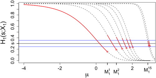
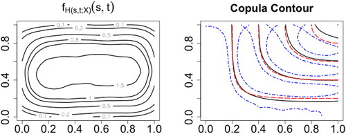
In contrast, when Y has an infinite range, for instance Poisson variables, $\widehat{C}(s,t;\beta )$ is a nonstandard estimator in the following aspects. First, for a fixed point (s, t), $H(s,t;\mathbf{X})$ is a noncontinuous variable. To illustrate, we assume that Y₁ follows the commonly used Poisson generalized linear model (GLM) with the log link, that is, $Y_1|X_1\sim \text{Poisson}\left(\hspace{0.17em}\text{exp}\hspace{0.17em}(X_1^{\prime }{\beta }_1)\right)$. Figure 1 shows $H_1(s;X_1)$ as a function of $\mu =X_1^{\prime }{\beta }_1$ (solid curves). In this example, for a fixed k, $F_1(k|X_1)$ is a monotone decreasing function of μ (dashed lines). From Figure 1, the curve of $H_1(s;X_1)$ is composed of continuous pieces from the curves of $F_1(k|X_1),k=0,\dots$. To formalize, denote $M_1^k$ as the jump point of $H_1(s;X_1)$ on the curve of $F_1(k|X_1)$, as in Figure 1. For example, when $\mu <M_1^1,F_1(0|X_1)$ is closest to s, and hence $H_1(s;X_1)=F_1(0|X_1)$ from its definition. When $\mu =M_1^1,F_1(0|X_1)$ and $F_1(1|X_1)$ are equidistant from s, and we define $H_1(s;X_1)$ as $F_1(1|X_1)$. While $M_1^1<\mu <M_1^2,F_1(1|X_1)$ is closest to s, and thus $H_1(s;X_1)=F_1(1|X_1)$. To generalize, it can be seen that (7) $$H_1(s;X_1)=F_1\left(k\right|X_1) \text{when} M_1^k\le \mu <M_1^{k+1},$$(7) and $M_1^0$ is set to be $-\infty$ for completion. Hence, the random variable $H_1(s;X_1)$ is a continuous function of μ almost everywhere except at a countable number of points under which s is in the middle of two grid points. Similar arguments apply to $H_2(t;X_2)$. We will further analyze the issue of discontinuity in Section 2.3. Because of these discontinuities, the proof for asymptotic properties of the estimator is not trivial.

Fig. 1 $H_1(s;X_1)$ (solid curve) as a function of $\mu =X_1^{\prime }{\beta }_1$ for Poisson GLM with the log link. Dashed curves: $F_1(k|X_1)$, from left to right $k=0,1,2,3,4,5,15$, and 16. The curve of $H_1(s;X_1)$ is composed of pieces from the curves of $F_1(k|X_1),k=0,\dots$. Horizontal lines: $s+ϵ,s$, and $s-ϵ$.

Second, $H(s,t;\mathbf{X})$ is a function of (s, t). That is, when estimating the copula at different points, we plug different variables into the kernel function, which differs from the setting of traditional nonparametric regression models. The dynamic scheme increases efficiency especially when the data are less discrete. This point will be demonstrated using a simulation study in the supplementary material.

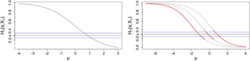
It should be emphasized that though we address the technical challenges associated with count outcomes, our methodological and theoretical results are applicable to general discrete data. Following the Poisson example in Figure 1, Figure 2 shows that $H_1(s;X_1)$ presents similar curves for binary and ordinal outcomes with commonly used regression models.

Fig. 2 $H_1(s;X_1)$ (solid curve) as a function of $\mu =X_1^{\prime }{\beta }_1$ for logistic regression (left panel) and ordinal regression with 4 levels (right panel). Dashed curves for right panel: $F_1(k|X_1)$, from left to right k = 0, 1, 2. Horizontal lines: $s+ϵ,s,s-ϵ$.

2.3 Asymptotic Behavior

In this section, we study the asymptotic properties of the copula estimator $\widehat{C}(s,t;\widehat{\beta })$ defined in Equation (6)(6) $$\widehat{C}(s,t;\beta )=\sum _{i=1}^n{W}_{\mathit{ni}}(s,t;{\mathbf{X}}_i,\beta )Y_i(\beta ),$$(6) . We first analyze $\widehat{C}(s,t;\beta )$, then plug in the estimator of β.

In the previous section, we demonstrated that marginally, for j = 1, 2, for a fixed k, $F_j(k|X_j)$ is a monotone decreasing function of a random location parameter ${\mu }_j=X_j^{\prime }{\beta }_j$. Hence, $F_j(k|X_j)$ is random with its own distribution function and, assuming continuity, a density. Let $f_{F_j(k|X_j)}$ denote the density of $F_j(k|X_j)$, and $f_{H_j(s;X_j)}$ is the density of $H_j(s;X_j)$. From the form of the estimator (6), the weights $W_{\mathit{ni}}(s,t;{\mathbf{X}}_i,\beta )$ relate to the density of $f_{H_j(s;X_j)}$ at s as $f_{H_j(s;X_j)}(s)$, and by transformation of random variables $$f_{H_j(s;X_j)}\left(s\right)=\sum _{k=0}^{\infty }{f}_{F_j\left(k\right|X_j)}\left(s\right).$$

Note for ordinal (binary) outcomes, the summation is up to the second largest possible value.

In contrast, the density of $H_j(s;X_j)$ at a point other than s, $f_{H_j(s;X_j)}(s+ϵ)$ has a different form from $f_{H_j(s;X_j)}(s)$ for $ϵ\ne 0$. Given ${\mu }_j=M_j^k$ defined in Equation (7)(7) $$H_1(s;X_1)=F_1\left(k\right|X_1) \text{when} M_1^k\le \mu <M_1^{k+1},$$(7) , denote the corresponding function value of $H_j(s;X_j)$ as ${\nu }_j^k$. For a small k such as $k\le 5$ in Figure 1, $|{\nu }_j^k-s|>ϵ$, that is, the jump point of $H_j(s;X_j)$ on the curve of $F_j(k|X_j)$ is outside the ϵ neighborhood of s. Hence, $f_{F_j(k|X_j)}$ contributes to $f_{H_j(s;X_j)}$ at $s+ϵ$ when applying transformation of random variables. While for large k such as k = 15, $|{\nu }_j^k-s|<ϵ$, and thus the density of $F_j(15|X_j)$ does not contribute to the density of $f_{H_j(s;X_j)}$ at $s+ϵ$. Therefore, in this example, (8) $$\sum _{k=0}^5{f}_{F_j\left(k\right|X_j)}(s+ϵ)\le f_{H_j(s;X_j)}(s+ϵ)<\sum _{k=0}^{\infty }{f}_{F_j\left(k\right|X_j)}(s+ϵ).$$(8)

That is, $f_{H_j(s;X_j)}$ is not smooth due to loss of $f_{F_j(k|X_j)}$ curves contributing to $f_{H_j(s;X_j)}$ at $s+ϵ$.

The nonsmoothness issue is less of a concern for finite range variables. When ϵ takes a small value ϵ_n which goes to 0, a finite number of jump points as in Figure 2 would be excluded from the small neighborhood of s. Therefore, they do not require following Lemma 2.1 and Assumption 2.1 which are made to handle the nonsmoothness issue for variables with infinite ranges.

The following lemma guarantees the summation on the left-hand side of Equation (8)(8) $$\sum _{k=0}^5{f}_{F_j\left(k\right|X_j)}(s+ϵ)\le f_{H_j(s;X_j)}(s+ϵ)<\sum _{k=0}^{\infty }{f}_{F_j\left(k\right|X_j)}(s+ϵ).$$(8) can be up to a large number $a_n(s)$ going to $\infty$, and $f_{H_j(s;X_j)}$ can be approximated by ${\sum }_{k=0}^{a_n(s)}{f}_{F_j(k|X_j)}$, which is continuous in the ϵ_n neighborhood of s.

Lemma 2.1.

There exists a sequence $a_n(s)$ going to infinity such that for all $k\le a_n(s),|{\nu }_j^k-s|>{ϵ}_n$, and thus $f_{H_j(s;X_j)}(s+{ϵ}_n)\ge {\sum }_{k=0}^{a_n(s)}{f}_{F_j(k|X_j)}(s+{ϵ}_n)$.

The proofs for this and other theoretical results can be found in the supplementary materials. Since there are countable jump points of $H_1(s;X_1)$ and ${ϵ}_n\to 0$, Lemma 2.1 can be satisfied by choosing right order of $a_n(s)$. Specifically, Lemma 2.1 is satisfied by choosing $a_n(s)$ to be $1/{ϵ}_n^2$ for Poisson and $1/{ϵ}_n$ for negative binomial distributions; see verifications in Yang (2017).

Extending our notation, denote the joint density of $\left(F_1(k_1|X_1),F_2(k_2|X_2)\right)$ as $f_{F_1(k_1|X_1),F_2(k_2|X_2)}$, and $f_{H(s,t;\mathbf{X})}$ as the density of $H(s,t;\mathbf{X})$. It can be seen (9) $$f_{H(s,t;\mathbf{X})}(s,t)=\sum _{k_1=0}^{\infty }\sum _{k_2=0}^{\infty }{f}_{F_1\left(k_1\right|X_1),F_2(k_2\left|X_2\right)}(s,t).$$(9)

Similar to the univariate case, the summation is up to the second largest possible values for outcomes with finite range. Recall $M_1^{a_n(s)}$ denotes the jump point of $H_1(s;X_1)$ on the curve of $F_1(a_n(s)|X_1)$ as in Equation (7)(7) $$H_1(s;X_1)=F_1\left(k\right|X_1) \text{when} M_1^k\le \mu <M_1^{k+1},$$(7) . The following assumption guarantees the non-smoothness of $f_{H(s,t;\mathbf{X})}$ is negligible by constraining the tail probability of μ_j.

Assumption 2.1.

Let $a_n(s)$ and $b_n(t)$ be sequences as in Lemma 2.1 for $H_1(s;X_1)$ and $H_2(t;X_2)$, respectively, then ${ϵ}_n^{-2}P({\mu }_1>M_1^{a_n(s)})\to 0$ and ${ϵ}_n^{-2}P({\mu }_2>M_2^{b_n(t)})\to 0$.

Assume we can interchange the derivatives and the limits, the partial derivatives of $f_{H(s,t;\mathbf{X})}(s,t)$ are $f_{H(s,t;\mathbf{X}),1}=\partial f_{H(s,t;\mathbf{X})}/\partial s$ and $f_{H(s,t;\mathbf{X}),2}=\partial f_{H(s,t;\mathbf{X})}/\partial t$. We make the following regularity assumption to ensure $f_{F_1(k_1|X_1),F_2(k_2|X_2)}$ is sufficiently smooth.

Assumption 2.2.

For fixed k₁ and k₂, $f_{F_1(k_1|X_1),F_2(k_2|X_2)}$ is twice continuously differentiable. The density$f_{H(s,t;\mathbf{X})}$ and its derivatives are bounded.

A necessary condition for Assumption 2.2 is that there exists a continuous regressor whose coefficient is not 0. When Y₁ and Y₂ follow Poisson distributions with means ${\lambda }_1=\hspace{0.17em}\text{exp}\hspace{0.17em}({\mu }_1)$ and ${\lambda }_2=\hspace{0.17em}\text{exp}\hspace{0.17em}({\mu }_2)$, Assumptions 2.1 and 2.2 are satisfied if ${\mathrm{E}}_{X_1}{\lambda }_1,{\mathrm{E}}_{X_2}{\lambda }_2$, and ${\mathrm{E}}_{\mathbf{X}}\sqrt{{\lambda }_1{\lambda }_2}$ are finite, and they hold for negative binomial distributions if ${\mathrm{E}}_{X_1}{\lambda }_1^2,{\mathrm{E}}_{X_2}{\lambda }_2^2$, and ${\mathrm{E}}_{\mathbf{X}}{\lambda }_1{\lambda }_2$ are finite. Therefore, if there are highly right-skewed covariates, log transformation is suggested. For binary and ordinal variables, Assumption 2.2 is satisfied given that the density of μ_j is twice continuously differentiable.

The copula is assumed to satisfy smoothness conditions, which guarantees the eligibility of approximating the copula value at a point using its neighborhood.

Assumption 2.3.

The copula C for $Y_1|X_1$ and $Y_2|X_2$ does not change with X. The copula is twice continuously differentiable, and the corresponding partial derivatives are bounded.

The first part of Assumption 2.3 is called “simplifying assumption” (Haff, Aas, and Frigessi 2010). Let V be a subset of ${(0,1)}^2$ such that for $(s,t)\in V,f_{H(s,t;\mathbf{X})}(s,t)>0$. Denote C₁, C₂, C₁₁, and C₂₂ as first and second order partial derivatives of C. Let the bandwidth ϵ_n satisfy that ${ϵ}_n\to 0$ and $n{ϵ}_n^2\to \infty$ as $n\to \infty$, and $n{ϵ}_n^6=O(1)$. Assume K is a symmetric and compact supported kernel function, and denote $R_2(K)=\int K{(u,v)}^2\mathrm{d}u\mathrm{d}v,{\kappa }_2=\int u^{2}K(u,v)\mathrm{d}u\mathrm{d}v$, we have the following property.

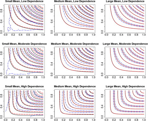
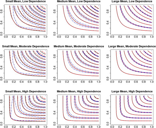
Fig. 3 Contour plots of the nonparametric estimator for Poisson outcomes under different scenarios with sample size 1000. The average of the estimator over 500 replications is given by the solid lines, while the dash-dot symbols give the corresponding $95\%$ confidence interval for every other copula value, and the dashed lines give the underlying copulas.

Theorem 2.1

(Consistency). Under Assumptions 2.1–2.3, for $(s,t)\in V$, $$\widehat{C}(s,t;\beta ){\to }_{p}C(s,t).$$

With further assuming C satisfies Lipschitz condition, we can have asymptotic normality and corresponding order of $\widehat{C}(s,t;\beta )$.

Assumption 2.4.

C satisfies Lipschitz condition of order 2, that is, there exists a constant α₁ such that for any $(a,b),(s,t)\in {(0,1)}^2$, $$\left|C(s,t)-C(a,b)\right|\le {\alpha }_1{\left|(s,t)-(a,b)\right|}^2.$$

Theorem 2.2

(Asymptotic normality). Under Assumptions 2.1–2.4, for $(s,t)\in V$, $$\begin{array}{c}\sqrt{n{ϵ}_n^2}\left(\widehat{C}(s,t;\beta )-C(s,t)-{\kappa }_2\zeta (s,t){ϵ}_n^2\right)\\ \hspace{1em}{\to }_{d}N\left(0,\frac{R_2\left(K\right)C(s,t)(1-C(s,t\left)\right)}{f_{H(s,t;\mathbf{X})}(s,t)}\right),\end{array}$$ where (10) $$\begin{array}{c}\zeta (s,t)=\frac{C_{11}(s,t)}{2}+\frac{C_{22}(s,t)}{2}+\frac{C_1(s,t)f_{H(s,t;\mathbf{X}),1}(s,t)}{f_{H(s,t;\mathbf{X})}(s,t)}\\ +\frac{C_2(s,t)f_{H(s,t;\mathbf{X}),2}(s,t)}{f_{H(s,t;\mathbf{X})}(s,t)}.\end{array}$$(10)

Therefore, the asymptotic mean squared error (AMSE), a commonly used measure of the quality of an estimator, for $\widehat{C}(·;\beta )$ at (s, t) is $$\text{AMSE}\left(\widehat{C}(s,t;\beta )\right)={\kappa }_2^2\zeta {(s,t)}^2{ϵ}_n^4+\frac{C(s,t)(1-C(s,t\left)\right)R_2\left(K\right)}{n{ϵ}_n^2{f}_{H(s,t;\mathbf{X})}(s,t)},$$ which converges to 0.

The following assumptions ensure the asymptotics hold when we plug the estimates of the marginal models into the copula estimator. When the parameters are set to be θ, we denote $H(s,t;\mathbf{X},\theta )$ as the corresponding perturbed probability integral transform.

Assumption 2.5

(Lipschitz condition). There exists a constant α₂ such that for all i, for bounded θ and $\beta$, when $\left|\theta -\beta \right|$ is small enough, $$\left|H(s,t;{\mathbf{X}}_i,\theta )-H(s,t;{\mathbf{X}}_i,\beta )\right|\le {\alpha }_2\left|\theta -\beta \right|$$ almost surely.

Note that this assumption is satisfied when Y₁ and Y₂ follow Poisson GLMs with the log link and bounded covariates.

Assumption 2.6.

$n^{1/2}(\widehat{\beta }-\beta )=O_p(1)$.

Theorem 2.3.

With Assumptions 2.1–2.6, for $(s,t)\in V$, $$\begin{array}{c}\sqrt{n{ϵ}_n^2}\left(\widehat{C}(s,t;\widehat{\beta })-C(s,t)-{\kappa }_2\zeta (s,t){ϵ}_n^2\right)\\ \hspace{1em}{\to }_{d}N\left(0,\frac{C(s,t)(1-C(s,t\left)\right)R_2\left(K\right)}{f_{H(s,t;\mathbf{X})}(s,t)}\right).\end{array}$$

That is, the AMSE of the copula estimator $\widehat{C}(s,t;\widehat{\beta })$ is same as when the margins are known.

Here are a few comments on the asymptotic results especially for count outcomes; the cases of binary and ordinal outcomes are rather trivial. First, the estimator behaves well with large marginal means under which $f_{H(s,t;\mathbf{X})}(s,t)$ is large. For illustration in one dimension, we use Figure 1 as an example, and without loss of generality, we focus on the fixed point s in the figure. When μ takes a small value, for instance -3, $H_j(s;X_j)=F_j(0|X_j)$ which is around 1 and not in a small neighborhood of s. While μ is larger, it is more likely that $H_j(s;X_j)$ is in the small neighborhood of s. That is, the density $f_{H_j(s;X_j)}(s)$ is large when μ is mostly distributed at large values. Intuitively, as μ gets large, the grid gets dense and the variable is more similar to a continuous random variable. Extending to two dimensions, when both margins have large means, the estimator performs well. We will demonstrate this point in Section 3 through simulated examples.

Second, when s is small, it requires large μ value for $F_j(k|X_j)$ to be in a small neighborhood of s. Since we constrain the tail probability of μ by Assumption 2.1, $f_{H_j(s;X_j)}(s)$ is small in this case. In other words, we have more effective observations when we estimate the copula at the right upper corner than the lower left corner.

Third, here we only provide the theoretical results of bivariate case. The estimator can be extended to higher dimensions naturally by adopting higher dimensional kernel functions with smaller order of convergence $\sqrt{n{ϵ}_n^d}$, where d is the number of dimensions. We include a three-dimensional simulation study in Section 3. An alternative is to build up the multivariate models through bivariate blocks, known as the vine copula structure (Panagiotelis, Czado, and Joe 2012).

2.4 Selection of Bandwidth

An important choice to be made is the bandwidth which is selected to balance the bias and variance of the estimator. In this section, we establish a data-driven selector for the bandwidth. The benchmark bandwidth is the minimizer of the integrated squared error (ISE). The ISE is considered to be a desirable criterion when one wants to measure how good an estimator is for a given dataset and is defined as (11) $$\text{ISE}\left(\widehat{C}(s,t;\widehat{\beta })\right)={\int }_{s,t}{\left(\widehat{C}(s,t;\widehat{\beta })-C(s,t)\right)}^2\mathrm{d}s\mathrm{d}t.$$(11)

Hence, a good estimator is supposed to have a small ISE value. However, in practice, C(s, t) is unknown. In this section, we propose a practical “plug-in” bandwidth selection rule. The independence copula is one natural choice to plug in Equation (11)(11) $$\text{ISE}\left(\widehat{C}(s,t;\widehat{\beta })\right)={\int }_{s,t}{\left(\widehat{C}(s,t;\widehat{\beta })-C(s,t)\right)}^2\mathrm{d}s\mathrm{d}t.$$(11) . Furthermore, motivated by the idea of working covariance in generalized estimating equations (Zeger and Liang 1986), we propose a procedure to replace C(s, t) by a “rule-of-thumb” estimator: a Frank copula estimated by maximum likelihood. We apply a Frank copula as the working copula for the following practical reasons. First, a Frank copula can capture a wide range of dependence including positive and negative dependence. Second, Frank copulas belong to the Archimedean family with a closed form of distribution functions and benefits of easy computation. There is no absolute justification for this choice. If there is prior information such as tail dependence, a more informative copula can be applied in our procedure.

The idea of “plug-in” has been widely applied for choosing smoothing parameters in kernel density estimation (Chiu 1991) and nonparametric regression with an odd number order of local polynomial (Ruppert, Sheather, and Wand 1995), in which optimal smoothing parameters are selected by minimizing an approximation to the mean integrated squared error or its asymptotic form. Nonetheless, the asymptotic mean integrated squared error of the proposed nonparametric estimator involves $f_{H(s,t;\mathbf{X})}(s,t)$ and its derivatives, as in Theorem 2.3. Since $f_{H(s,t;\mathbf{X})}(s,t)$ is not a typical density function, its approximation takes extra efforts than plugging in a parametric density function. In addition, the estimation of the derivatives of $f_{H(s,t;\mathbf{X})}(s,t)$ is challenging and has a smaller order of convergence. We also avoid using cross-validation due to its computational burden. Because $H(s,t;\mathbf{X})$ varies with (s, t), the typical setting of generalized cross-validation, which is an approximation to cross-validation and commonly applied for bandwidth selection in nonparametric regression, is violated.

We conduct a simulation study to assess the proposed bandwidth selector by comparing it with the benchmark selector minimizing the ISE values. The detailed results are included in the supplementary materials. Overall, the proposed selector performs quite satisfactorily under different scenarios.

3 Simulation Study

In this section, we evaluate the overall ability of the proposed estimator to identify a copula for different types of data under various scenarios. In addition, we explore our nonparametric estimator working as a diagnostic tool for choosing a parametric copula.

3.1 Simulation Study Design

The simulations are conducted under scenarios with combinations of different levels of dependence and discreteness in margins using the following algorithm. With a copula C and marginal models $F_j,j=1,2$ assumed,

1. Draw a bivariate uniform random variables from C, that is, $U_i=(U_{i1},U_{i2})\sim C$. Do this independently for $i=1,\dots ,n$. Note that the copula does not depend on covariates (a “simplifying assumption”).

2. Simulate covariates $(X_{\mathit{ij}}),i=1,\dots ,n,j=1,2$. Construct the jth marginal distribution function using covariates $(X_{\mathit{ij}})$ and assumed marginal parameters (β_j), that is, $$F_{\mathit{ij}}\left(z\right)=F_j\left(z\right|X_{\mathit{ij}}),j=1,2.$$

3. Obtain the jth discrete outcome by evaluating the uniform random variable at the inverse of the marginal distribution function, that is, $$Y_{\mathit{ij}}=F_{\mathit{ij}}^{(-1)}\left(U_{\mathit{ij}}\right).$$

For count variables, we demonstrate explicit results for Poisson outcomes as an example. The results of negative binomial variables are included in the supplementary materials from which we see similar patterns. Marginally, for j = 1, 2, the mean of the Poisson variable is based on the function $\mathrm{E}(Y_j|X_j)={\lambda }_j=\hspace{0.17em}\text{exp}\hspace{0.17em}({\beta }_{j0}+X_j{\beta }_{j1})$, where $X_1\sim N(0,1),X_2\sim N(0,1)$, independently. As indicated in Nikoloulopoulos (2013), it is more problematic to apply copulas when data are highly discrete with large probability of ties. Hence, we consider three marginal scenarios to explore the influence of the discreteness on the estimator. When λ_j is small, Y_j takes on a small number of values with high level of discreteness, while Y_j behaves analogously to a continuous variable with large λ_j. Parameters ${\beta }_{j0},j=1,2$ are allowed to vary to obtain different marginal mean levels:

• Small mean: ${\beta }_{10}=-2,{\beta }_{11}=2,{\beta }_{20}=-2$, and ${\beta }_{21}=1.5$.

• Medium mean: ${\beta }_{10}=0,{\beta }_{11}=2,{\beta }_{20}=0$, and ${\beta }_{21}=1.5$.

• Large mean: ${\beta }_{10}=5,{\beta }_{11}=2,{\beta }_{20}=5$, and ${\beta }_{21}=1.5$.

We also consider binary outcomes and let $F_j(0|X_j)=1/\left(1+\hspace{0.17em}\text{exp}\hspace{0.17em}(X_j^{\prime }{\beta }_j)\right)$, j = 1, 2, where $X_1\sim N(0,1),X_2\sim N(0,1)$ independently and ${\beta }_1=1.5,{\beta }_2=1$.

Meanwhile, three levels of dependence are considered. To compare across different copulas, we quantify dependence of C using Kendall’s τ as 0.07 for low dependence, 0.2 for moderate dependence, and 0.6 for high dependence, respectively. We also conducted the analysis on negative correlated data and found out it is the level instead of the sign of the correlation that influences the results mostly. We use sample sizes n = 1000 and n = 5000. The number of replications in each simulation is 500, and the Epanechnikov kernel is used throughout.

3.2 Finite-Sample Performance

We first assess the finite sample performance of our estimator under different scenarios. Here we employ Gaussian copulas as the underlying dependence models. Correspondingly, the parameter of the Gaussian copula under low, moderate, and high dependence are 0.1, 0.3, and 0.8. There are many possibilities for the dependence models. Although their results are not reported here, we can draw consistent conclusions. With simulated data, we first fit their marginal models and then plug the estimates in the copula estimator (6).

3.2.1 Count

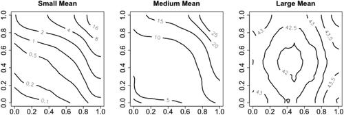
Figure 3 displays the proposed estimator for Poisson outcomes under different scenarios with sample size n = 1000. For clarification, the corresponding confidence intervals are given for every other copula value. The leftmost plots correspond to the cases with small marginal means. We can see both bias and variance are large under high discreteness level. This is consistent with the theoretical results in Section 2.3. Figure 4 includes the contour plots of $f_{H(s,t;\mathbf{X})}(s,t)$ for $(s,t)\in {(0,1)}^2$. In the small mean scenario, the values of $f_{H(s,t;\mathbf{X})}(s,t)$ are small, and thus the number of effective observations with positive weights in Equation (6)(6) $$\widehat{C}(s,t;\beta )=\sum _{i=1}^n{W}_{\mathit{ni}}(s,t;{\mathbf{X}}_i,\beta )Y_i(\beta ),$$(6) is small. As a result, large bias and variance are expected, especially at the lower left corner, which is getting out of the V area of Theorem 2.3.

Fig. 4 Contour plots of $f_{H(s,t;\mathbf{X})}(s,t)$ for Poisson outcomes under different marginal mean levels.

As the marginal means increase to the medium level, as displayed in the middle column of Figure 3, it is clear that the accuracy of the estimator improves with smaller bias and variance as a result of larger $f_{H(s,t;\mathbf{X})}(s,t)$ values from Figure 4. When the marginal means increase to the large scenario (right column of Figure 3), the estimator appears to perform well with negligible bias and variance. Indeed, as the grid points become dense, the estimator behaves seemingly with order of convergence $n^{-1/2}$.

By comparing across different levels of dependence corresponding to the rows in Figure 3, we can conclude the level of dependence is less influential on the performance of the copula estimator than the discreteness. Figure 5 shows the results with sample size n = 5000. As anticipated, the bias and variance are smaller with larger sample size. This phenomenon suggests the identification of copulas even when outcomes are highly discrete is possible if the sample size is sufficiently large.

Fig. 5 Contour plots of the nonparametric estimator for Poisson outcomes under different scenarios with sample size 5000.

Correspondingly, the results are summarized numerically in Table 1. We quantify the performance of the estimator using the ISE defined in Equation (11)(11) $$\text{ISE}\left(\widehat{C}(s,t;\widehat{\beta })\right)={\int }_{s,t}{\left(\widehat{C}(s,t;\widehat{\beta })-C(s,t)\right)}^2\mathrm{d}s\mathrm{d}t.$$(11) . As an example, when the sample size is n = 1000, over the 500 replications, the average ISE of the nonparametric estimator is $2.865\times {10}^{-3}$ with a standard deviation $2.081\times {10}^{-3}$ for the case with small marginal means and low dependence. Consistent with Figures 3 and 5, the level of discreteness plays an important role on the performance of the nonparametric estimator, which is reflected in the ISE values. The nonparametric estimator performances better as the marginal means and the sample size increase. We also carry out simulations with mixed marginal discreteness levels in the supplementary materials, whose overall performance lies between the corresponding two cases with identical marginal mean levels.

Table 1 ISE values for Poisson examples under different scenarios (multiplied by 1000).

		n = 1000		n = 5000
Marginal mean	Dependence	Average	SD	Average	SD
Small	Low	2.865	2.081	0.857	0.311
	Moderate	3.061	2.233	0.878	0.334
	High	3.547	2.652	0.974	0.429
Medium	Low	0.331	0.118	0.107	0.030
	Moderate	0.330	0.125	0.101	0.030
	High	0.352	0.150	0.103	0.031
Large	Low	0.088	0.040	0.018	0.009
	Moderate	0.088	0.040	0.018	0.009
	High	0.091	0.047	0.019	0.010

3.2.2 Binary

For binary outcomes, with high level of discreteness, it is difficult to estimate the dependence structure; this difficulty is clearly demonstrated in Figure 6. As the estimator performs comparably across different levels of dependence, here we only employ Gaussian copula with high dependence as the underlying model. The values of $f_{H(s,t;\mathbf{X})}(s,t)$ are small especially near boundary as shown in the left panel. Thus, the estimator, which coincides with the Nadaraya–Watson estimator in this case, has large bias and variance reflected in the right panel of Figure 6 as well as large ISE values summarized in the supplementary materials.

Fig. 6 Left panel: contour plot of $f_{H(s,t;\mathbf{X})}(s,t)$ for binary outcomes. Right panel: contour plot of the nonparametric estimator for binary outcomes with sample size 5000.

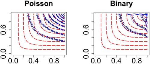
To illustrate that the empirical copula estimator (4) is not a consistent copula estimator for discrete outcomes, the contour plots of the empirical copula estimator compared with the underlying copulas for two simulated examples, Poisson outcomes with medium marginal means and binary outcomes with high dependence and sample size 5000, are displayed in Figure 7, which clearly confirms the necessity of alternative ways of estimating the copula. We can see that under the same settings the proposed estimator provides more reasonable fitting as the middle panel in the bottom row of Figure 5 and right panel of Figure 6.

Fig. 7 Contour plots of the empirical copula estimator (solid curve) with its confidence interval (dash-dot symbols) compared with the underlying copulas (dashed lines).

3.2.3 Higher Dimension

As discussed in Section 2.3, our estimator can be extended to higher dimensions naturally. We conduct simulations with three dimensional Poisson variables at a high dependence level, and Table 2 summarizes the results numerically. Comparing Table 2 with the corresponding cells in Table 1, we see that under small mean level, the estimator suffers from the curse of dimensionality which is a well-known problem in nonparametric regression. Interestingly, when the marginal means are large, the curse of dimensionality is mitigated, as the ISE value of the three-dimensional estimator is comparable to the bivariate estimator. An intuitive reason is that the variables behave analogously to continuous outcomes in this case.

Table 2 ISE of three-dimensional estimator for Poisson outcomes under high dependence with sample size 5000 (multiplied by 1000).

Marginal Mean	Average	SD
Small	2.500	1.408
Medium	0.143	0.042
Large	0.017	0.008

3.3 Copula Specification and Diagnosis

There are few approaches available for copula specification and diagnosis in discrete cases. In practice, overall goodness-of-fit statistics, such as AIC, BIC, and likelihood, are used to choose the best model among candidates. Vuong’s test (Vuong 1989) can be applied to further compare if the models are statistically significantly different. However, these methods are not diagnostic for adequacy of fit and do not suggest improvements. The classical way of comparing expected and observed counts is infeasible when there are many large observations and hard to present when the dimension is greater than two.

The proposed nonparametric estimator can serve as a specification and diagnostic tool for selecting a parametric copula. We now explore the usage under different scenarios. For each of the simulations, given the generated data, we first fit the marginal models. Then, we plug the marginal estimates in Equation (6)(6) $$\widehat{C}(s,t;\beta )=\sum _{i=1}^n{W}_{\mathit{ni}}(s,t;{\mathbf{X}}_i,\beta )Y_i(\beta ),$$(6) to obtain our nonparametric estimator. Meanwhile, different parametric copulas are fit through MLE. Finally, we compare the parametric copulas with our nonparametric estimator.

To measure the distance between the fitted parametric copulas with the nonparametric copula estimator, we use the L₂-norm distance (12) $$d\left(\widehat{C}\right(·;\widehat{\beta }),{\tilde{C}}_{\widehat{\theta }})={\int }_{s,t}\left(\widehat{C}\right(s,t;\widehat{\beta })-{\tilde{C}}_{\widehat{\theta }}(s,t){)}^2\mathrm{d}s\mathrm{d}t,$$(12) where $\widehat{C}(·;\widehat{\beta })$ is the proposed nonparametric estimator, and ${\tilde{C}}_{\widehat{\theta }}$ is the parametric copula. The parametric copulas with good fitting are supposed to be close to our nonparametric estimator with small distances.

We generated the data using Gaussian (no tail dependencies), Clayton (lower tail dependence), and Joe (upper tail dependence) copulas to explore the impact of tail dependence. The detailed graphical and numerical results are provided in the supplementary material due to space limitations. To summarize, first, the selection of copula is more important with large marginal means and high dependence. Second, overall, our nonparametric estimator is likely to exclude copulas with wrong tail behaviors, especially those with opposite tail dependence structures of the underlying model. In the situations where it seems ambiguous between copulas, we suggest expanding the candidate pool.

4 Data Example

To illustrate the nonparametric estimator on real data, we use our model to investigate the dependence of insurance claim frequencies across different business lines using a unique dataset from the LGPIF in the state of Wisconsin.

The LGPIF was established to provide property insurance for local government entities that include counties, cities, towns, villages, school districts, fire departments, and other miscellaneous entities. The fund provides different types of coverage including government buildings, vehicles, and equipments. For example, a county may need coverage for the buildings (and their contents) that it owns as well as coverage for its automobiles and trucks. The LGPIF operates similarly to a typical insurer, hence the data provide a good example for multiline insurance companies encountered in practice.

4.1 Data Summary

We focus on joint modeling of BC and MV insurance of the LGPIF. Table 3 shows the total number of policies for each coverage type in the dataset for years 2006–2010. Jointly, there are 2170 observations with both coverages.

Table 3 Empirical numbers of observations.

	Total	0	1	2	3	4	5	>5
BC	5660	3976	997	333	136	76	31	111
MV	2175	1511	314	116	53	36	21	124
Joint	2170

Potential rating variables, covariates, are displayed in Table 4. Here coverage and deductible are continuous covariates which is essential for copula estimation.

Table 4 Description and summary statistics of covariates.

Variable	Description	Mean
TypeCity	=1 if entity type is city	0.140
TypeCounty	=1 if entity type is county	0.058
TypeSchool	=1 if entity type is school	0.282
TypeTown	=1 if entity type is town	0.173
TypeVillage	=1 if entity type is village	0.237
TypeMisc	=1 if entity type is other	0.110
NoClaimCreditBC	=1 if no building and content claims
	in prior year given BC coverage	0.328
NoClaimCreditMV	=1 if no MV claims
	in prior year given MV coverage	0.054
lnCoverageBC	Coverage of BC line in logarithmic	2.119
	millions of dollars given BC coverage	(2.000)
lnCoverageMV	Coverage of MV line in logarithmic	−0.798
	millions of dollars given MV coverage	(1.626)
lnDeductBC	BC deductible level in logarithmic	7.155
	millions of dollars given BC coverage	(1.174)

Preliminary dependence measures for discrete claim frequencies can be obtained using simple correlation statistics such as Kendall’s τ and Spearman’s ρ. Table 5 shows the correlations between the frequencies of the two coverages. Note that these dependence measures in Table 5 are calculated before controlling for the effects of explanatory variables and should be taken with caution due to the following reasons. First, as discussed in Denuit and Lambert (2005), the definitions of Kendall’s τ and Spearman’s ρ do not take the probability of ties into account and are not free of margins. Second, the large values of the dependencies may be due to correlations in the covariates. We will further quantify the correlations using likelihood-based estimation after controlling the effects of covariates in Section 4.3.

Table 5 Correlations between frequencies of claims.

Kendall’s τ	Spearman’s ρ
0.361	0.402

4.2 Marginal Models

From Table 3, it can be seen that the BC line contains a large number of zeros and a significant amount of ones. This motivates the usage of zero-one-inflated Poisson models in Frees, Lee, and Yang (2016). The distribution function can be expressed as $$F_j\left(k\right|X_j,{\beta }_j)=\{\begin{array}{cc}{\pi }_{j0}+(1-{\pi }_{j0}-{\pi }_{j1})\hspace{0.17em}\text{exp}\hspace{0.17em}(-{\lambda }_j)& k=0,\\ {\pi }_{j0}+{\pi }_{j1}+(1-{\pi }_{j0}-{\pi }_{j1})\sum _{i=0}^k{\lambda }_j^i\hspace{0.17em}\text{exp}\hspace{0.17em}(-{\lambda }_j)\frac{1}{i!}& k>0.\end{array}$$

Here, we employ the marginal models chosen in Frees, Lee, and Yang (2016) in which expected and observed counts were compared. For BC line, the zero-one-inflated Poisson model outperformed the other methods, while for MV line, the negative binomial model was selected. The coefficients for the selected models are in Table 6. We address that it is the benefit of employing copula regression models that the marginal models can be freely specified.

Table 6 Marginal coefficients.

		BC (0-1 inflated Poisson)		MV (Negative Binomial)
	Variable Name	Coef.	SE	Coef.	SE
Count	(Intercept)	−1.540	0.125	−0.929	0.109
	lnCoverage	0.751	0.023	0.708	0.036
	lnDeduct	−0.020	0.017
	NoClaimCredit	−0.395	0.131	−0.370	0.146
	TypeCity	−0.143	0.079	0.231	0.149
	TypeCounty	−0.250	0.087	1.518	0.132
	TypeMisc	−0.195	0.179	−0.352	0.301
	TypeSchool	−1.157	0.085	0.651	0.131
	TypeTown	0.186	0.175	−1.085	0.244
	size			1.428	0.139
Zero	(Intercept)	−4.755	0.448
	lnCoverage	−0.580	0.078
	lnDeduct	0.879	0.062
	NoClaimCredit	0.536	0.280
One	(Intercept)	−5.533	0.639
	lnCoverage	−0.047	0.094
	lnDeduct	0.577	0.084
	NoClaimCredit	0.300	0.353

4.3 Copula Estimation

Given well-fitting marginal models, now we are in a position to conduct dependence analysis. We focus on the 2170 policies with both BC and MV coverages. The nonparametric estimator is fit with bandwidth selected by the process explored in Section 2.4. The fitted nonparametric copulas are displayed in Figure 8 as the solid curves.

Fig. 8 Contour plot of the nonparametric estimator (solid) and its confidence intervals (dotted) compared with parametric copulas contours (dashed).

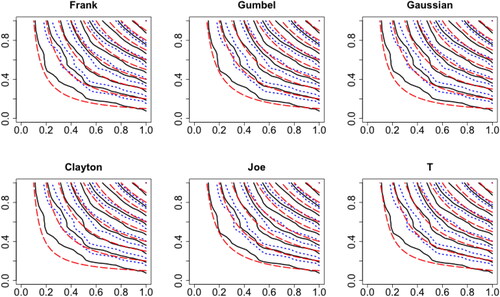
To address the practical issue of parametric copula selection, we compare the nonparametric estimator with different commonly used parametric copulas fit through MLE. Table 7 includes the parameters of different copulas. When the parameters are transformed to Kendall’s τ, it is not surprising that the dependence is weaker than the raw dependence from Table 5 that was computed before introducing covariates, and it is comparable to the low dependence scenario of our simulation. Figure 8 shows the graphical comparisons between different parametric copulas with the nonparametric estimator. As in Section 3.3, it is difficult to distinguish among different copulas when the dependence is weak. From Figure 8, we are only able to conclude that the Clayton copula does not fit well.

Table 7 Parameters from different parametric copulas.

	Estimate	SE	Kendall’s τ
Gumbel	1.040	0.015	0.038
Joe	1.042	0.018	0.024
T(df = 4)	0.072	0.038	0.046
Frank	0.718	0.221	0.079
Gaussian	0.125	0.033	0.079
Clayton	0.223	0.075	0.100

We further summarize the discrepancies numerically using the distance defined in Equation (12)(12) $$d\left(\widehat{C}\right(·;\widehat{\beta }),{\tilde{C}}_{\widehat{\theta }})={\int }_{s,t}\left(\widehat{C}\right(s,t;\widehat{\beta })-{\tilde{C}}_{\widehat{\theta }}(s,t){)}^2\mathrm{d}s\mathrm{d}t,$$(12) in Table 8. The Frank, Gaussian, and Clayton copulas can be excluded due to their large discrepancies. The performance of the t, Gumbel, and Joe copulas seem similar, which suggests that there is upper tail dependence in this dataset. To take the uncertainty into account, we do bootstrap with the number of replications as 500 to obtain the standard errors of the distances. Since the standard errors are comparable, given the smallest mean distance in Table 8, the Gumbel copula seems to best describe the dependence.

Table 8 Distances $d(\widehat{C}(·;\widehat{\beta }),{\tilde{C}}_{\widehat{\theta }})$ of different parametric copulas (multiplied by 1000).

	Gumbel	Joe	t	Frank	Gaussian	Clayton
Estimate	0.633	0.635	0.646	0.711	0.701	0.885
SE	0.240	0.251	0.240	0.239	0.237	0.265

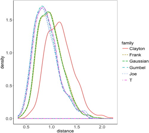
Since the distances of parametric copulas with our nonparametric estimator may not be normally distributed, standard errors may not be informative enough to quantify the uncertainty. Figure 9 displays the distribution of the distances of different copula families constructed from bootstrap samples. The Joe, Gumbel, and t copulas appear better than the rest in the sense that their distances are mostly distributed around small values.

Fig. 9 Density plot of the distances (multiplied by 1000) of different parametric copulas.

5 Summary and Concluding Remarks

In this article, we considered modeling multivariate discrete outcomes with copulas. We explored dependence modeling in the practical regression settings. Our main contribution is the proposal of a nonparametric copula estimator to specify the dependence structure under discreteness when the premises of the methodologies under continuity are violated. We also showed its asymptotic properties. Using a simulation study, we concluded that first, the estimator behaves better with small bias and variance when the data are less discrete, which is consistent with the theoretical results. Second, when used as a diagnostic tool, the nonparametric estimator can exclude false models easily when the dependence is high and the discreteness level is low. The data analysis suggested in the LGPIF dataset, there is upper tail dependence between the claim frequencies from BC coverage and MV coverage.

We acknowledge that many potential improvements can be made for our study. In this article, we applied the local average approach. Local polynomial estimators can be explored to reduce bias on the boundary. In addition, the bandwidth selector, we proposed chooses a global bandwidth. Since for our estimator, we have more observations at the right upper corner than the lower left corner, the variable bandwidth in Fan and Gijbels (1995) might be applied. These are areas for our future work.

Supplementary Materials

The supplementary materials include proofs for theoretical results in Section 2.3 and detailed simulation results for Sections 2.4, 3.2, and 3.3.

Acknowledgments

The authors are grateful to the reviewers for insightful comments leading to an improved article. The work of the first two authors (Yang and Frees) was partially funded by a Society of Actuaries’ Center of Actuarial Excellence Grant.

References

- Aitchison, J., and Ho, C. (1989), “The Multivariate Poisson-Log Normal Distribution,” Biometrika, 76, 643–653. DOI: 10.1093/biomet/76.4.643.
- Bermúdez, L., and Karlis, D. (2011), “Bayesian Multivariate Poisson Models for Insurance Ratemaking,” Insurance: Mathematics and Economics, 48, 226–236. DOI: 10.1016/j.insmatheco.2010.11.001.
- Brown, C. E. (1998), “Multivariate Probit Analysis,” in Applied Multivariate Statistics in Geohydrology and Related Sciences, Berlin: Springer, pp. 167–169.
- Chen, S. X., and Huang, T.-M. (2007),“Nonparametric Estimation of Copula Functions for Dependence Modelling,” Canadian Journal of Statistics, 35, 265–282. DOI: 10.1002/cjs.5550350205.
- Chib, S., and Winkelmann, R. (2001), “Markov chain Monte Carlo Analysis of Correlated Count Data,” Journal of Business & Economic Statistics, 19, 428–435. DOI: 10.1198/07350010152596673.
- Chiu, S.-T. (1991) “Bandwidth Selection for Kernel Density Estimation,” The Annals of Statistics, 19, 1883–1905. DOI: 10.1214/aos/1176348376.
- Cox, D. R., and Snell, E. J. (1968), “A General Definition of Residuals,” Journal of the Royal Statistical Society, Series B, 30, 248–275. DOI: 10.1111/j.2517-6161.1968.tb00724.x.
- Deheuvels, P. (1979), “La Fonction de Dépendance Empirique et ses Propriétés. Un Test Non paramétrique d’Indépendance,” Acad. Roy. Belg. Bull. Cl. Sci.(5), 65, 274–292.
- Denuit, M. and Lambert, P. (2005), “Constraints on Concordance Measures in Bivariate Discrete Data,” Journal of Multivariate Analysis, 93, 40–57. DOI: 10.1016/j.jmva.2004.01.004.
- Fan, J., and Gijbels, I. (1995), “Adaptive Order Polynomial Fitting: Bandwidth Robustification and Bias Reduction,” Journal of Computational and Graphical Statistics, 4, 213–227. DOI: 10.2307/1390848.
- Fermanian, J. D., and Scaillet O. (2003). “Nonparametric estimation of copulas for time series,” Journal of Risk, 5, 25–54. DOI: 10.21314/JOR.2003.082.
- Frees, E. W., Jin, X., and Lin, X. (2013), “Actuarial Applications of Multivariate Two-Part Regression Models,” Annals of Actuarial Science, 7, 258–287. DOI: 10.1017/S1748499512000346.
- Frees, E. W., Lee, G., and Yang, L. (2016), “Multivariate Frequency-Severity Regression Models in Insurance,” Risks, 4, 1-36. DOI: 10.3390/risks4010004.
- Frees, E. W., and Valdez, E. A. (1998), “Understanding Relationships Using Copulas,” North American Actuarial Journal, 2, 1–25. DOI: 10.1080/10920277.1998.10595667.
- Genest, C., and Nešlehová, J. (2007), “A Primer on Copulas for Count Data,” Astin Bulletin, 37, 475–515. DOI: 10.1017/S0515036100014963.
- Genest, C., Nikoloulopoulos, A. K., Rivest, L.-P., and Fortin, M. (2013), “Predicting Dependent Binary Outcomes Through Logistic Regressions and Meta-Elliptical Copulas,” Brazilian Journal of Probability and Statistics, 27, 265–284. DOI: 10.1214/11-BJPS165.
- Haff, I. H., Aas, K., and Frigessi, A. (2010), “On the Simplified Pair-Copula Construction–Simply Useful or Too Simplistic?” Journal of Multivariate Analysis, 101, 1296–1310. DOI: 10.1016/j.jmva.2009.12.001.
- Jiryaie, F., Withanage, N., Wu, B., and De Leon, A. (2016), “Gaussian Copula Distributions for Mixed Data, With Application in Discrimination,” Journal of Statistical Computation and Simulation, 86, 1643–1659. DOI: 10.1080/00949655.2015.1077386.
- Joe, H. (1993) “Parametric Families of Multivariate Distributions With Given Margins,” Journal of Multivariate Analysis, 46, 262–282. DOI: 10.1006/jmva.1993.1061.
- Joe, H. (2014), Dependence Modeling with Copulas: CRC Press.
- Johnson, N. L., Kotz, S., and Balakrishnan, N. (1997), Discrete Multivariate Distributions, Vol. 165: Wiley New York.
- Li, D. X. (1999), “On Default Correlation: A Copula Function Approach,” available at SSRN 187289.
- Li, B., and Genton, M. G. (2013), “Nonparametric Identification of Copula Structures,” Journal of the American Statistical Association, 108, 666–675. DOI: 10.1080/01621459.2013.787083.
- McCullagh, P., and Nelder, J. A. (1989), Generalized Linear Models (Vol. 37). London: CRC Press.
- McCulloch, C. E., and Neuhaus, J. M. (2005), Generalized Linear Mixed Models, Hoboken: Wiley.
- Muthén, B. (1979), “A Structural Probit Model With Latent Variables,” Journal of the American Statistical Association, 74, 807–811.
- Nelsen, R. B. (2006), An Introduction to Copulas, New York: Springer Science & Business Media.
- Nikoloulopoulos, A. K. (2013), “Copula-Based Models for Multivariate Discrete Response Data,” in Copulae in Mathematical and Quantitative Finance, eds. P. Jaworski, F. Durante, and W. K. Härdle, Berlin: Springer, pp. 231–249.
- Nikoloulopoulos, A. K., and Karlis, D. (2008), “Multivariate Logit Copula Model With an Application to Dental Data,” Statistics in Medicine, 27, 6393–6406. DOI: 10.1002/sim.3449.
- Nikoloulopoulos, A. K., and Karlis, D. (2009), “Modeling Multivariate Count Data Using Copulas,” Communications in Statistics-Simulation and Computation, 39, 172–187.
- Omelka, M., Gijbels, I., and Veraverbeke, N. (2009), “Improved Kernel Estimation of Copulas: Weak Convergence and Goodness-of-Fit Testing,” The Annals of Statistics, 37, pp. 3023–3058. DOI: 10.1214/08-AOS666.
- Panagiotelis, A., Czado, C., and Joe, H. (2012), “Pair Copula Constructions for Multivariate Discrete Data,” Journal of the American Statistical Association, 107, 1063–1072. DOI: 10.1080/01621459.2012.682850.
- Ruppert, D., Sheather, S. J., and Wand, M. P. (1995), “An Effective Bandwidth Selector for Local Least Squares Regression,” Journal of the American Statistical Association, 90, 1257–1270. DOI: 10.1080/01621459.1995.10476630.
- Scaillet, O., and Fermanian, J.-D. (2002), “Nonparametric Estimation of Copulas for Time Series,” FAME Research Paper.
- Shi, P., and Valdez, E. A. (2014), “Multivariate Negative Binomial Models for Insurance Claim Counts,” Insurance: Mathematics and Economics, 55, 18–29. DOI: 10.1016/j.insmatheco.2013.11.011.
- Shih, J. H., and Louis, T. A. (1995), “Inferences on the Association Parameter in Copula Models for Bivariate Survival Data,” Biometrics, 1384–1399. DOI: 10.2307/2533269.
- Sklar, M. (1959), Fonctions de Répartition À N Dimensions et Leurs Marges, Université Paris 8.
- Song, P. X.-K. (2007), Correlated Data Analysis: Modeling, Analytics, and Applications, Springer Science & Business Media.
- Song, P. X.-K., Li, M., and Yuan, Y. (2009), “Joint Regression Analysis of Correlated Data using Gaussian Copulas,” Biometrics, Vol. 65, pp. 60–68. DOI: 10.1111/j.1541-0420.2008.01058.x.
- Vuong, Q. H. (1989), “Likelihood Ratio Tests for Model Selection and Non-Nested Hypotheses,” Econometrica, 57, 307–333. DOI: 10.2307/1912557.
- Winkelmann, R. (2000), “Seemingly Unrelated Negative Binomial Regression,” Oxford Bulletin of Economics and Statistics, 62, 553–560. DOI: 10.1111/1468-0084.00188.
- Yang, L. (2017), “Copula Regression With Discrete Outcomes,” Ph.D. dissertation, University of Wisconsin–Madison.
- Yang, X., Frees, E. W., and Zhang, Z. (2011), “A Generalized Beta Copula With Applications in Modeling Multivariate Long-Tailed Data,” Insurance: Mathematics and Economics, 49, 265–284. DOI: 10.1016/j.insmatheco.2011.04.007.
- Zeger, S. L., and Liang, K.-Y. (1986), “Longitudinal Data Analysis for Discrete and Continuous Outcomes,” Biometrics, 42, 121–130.
- Zilko, A. A., and Kurowicka, D. (2016), “Copula in a Multivariate Mixed Discrete–Continuous Model,” Computational Statistics & Data Analysis, 103, 28–55. DOI: 10.1016/j.csda.2016.02.017.